Unfolding Semantics of the Untyped Î»-Calculus with letrec

arXiv:1610.05954v1 [cs.PL] 19 Oct 2016

Dissertation:

Unfolding Semantics of the Untyped λ-Calculus with letrec

Jan Rochel

defended on June 20, 2016 online version, revision: October 20, 2016

Dedication: Gewidmet meiner ehemaligen Klavierlehrerin Eva-Maria Rieckert, die mir Musik auf eine Weise vermittelte, die mich bis heute u ¨ber das Musizieren hinaus pr¨ agt.

Promotoren:

Copromotor:

Prof.dr. S. D. Swierstra Prof.dr. V. van Oostrom

Dr. C. Grabmayer

Unfolding Semantics of the Untyped λ-Calculus with letrec Ontvouwingssemantiek van de ongetypeerde λ-calculus met letrec (met een samenvatting in het Nederlands)

Proefschrift ter verkrijging van de graad van doctor aan de Universiteit Utrecht op gezag van de rector magnificus, prof.dr. G.J. van der Zwaan, ingevolge het besluit van het college voor promoties in het openbaar te verdedigen op maandag 20 juni 2016 des middags te 2.30 uur

door

Jan Rochel

geboren op 20 juli 1984 te Bretten, Duitsland

Dit proefschrift werd (mede) mogelijk gemaakt met financiële steun van de Nederlandse Organisatie voor Wetenschappelijk Onderzoek (NWO).

Contents Contents

iii

Preface Abstract . . . . . . . . . . . . . . . . . . . . . . . . . . . . . . . . . . . . .

v vi

0 λletrec and Unfolding 0.1 Introduction . . . . . . . . . . . . . . . . . . . . . 0.2 λ-terms and λletrec -terms – informal . . . . . . . 0.3 Unfolding λletrec -terms – informal . . . . . . . . 0.4 Preliminaries . . . . . . . . . . . . . . . . . . . . 0.5 λ-terms and λletrec -terms – CRS formalisation . 0.6 Unfolding Rules – CRS formalisation . . . . . . 0.7 Unfolding Semantics of λletrec . . . . . . . . . . .

. . . . . . .

. . . . . . .

. . . . . . .

. . . . . . .

. . . . . . .

. . . . . . .

. . . . . . .

. . . . . . .

. . . . . . .

1 2 5 6 11 12 13 18

1 Expressibility in λletrec 1.1 Overview . . . . . . . . . . . . . . . . . . . . . . . . . . 1.2 Introduction . . . . . . . . . . . . . . . . . . . . . . . . 1.3 Preliminaries . . . . . . . . . . . . . . . . . . . . . . . 1.4 Regular and strongly regular λ-terms . . . . . . . . . 1.5 Observing λletrec -terms by their generated subterms 1.6 Proving regularity and strong regularity . . . . . . . 1.7 Binding–Capturing Chains . . . . . . . . . . . . . . . 1.8 Expressibility by terms in λletrec . . . . . . . . . . . . 1.9 λ-transition-graphs . . . . . . . . . . . . . . . . . . . . 1.10 Summary . . . . . . . . . . . . . . . . . . . . . . . . .

. . . . . . . . . .

. . . . . . . . . .

. . . . . . . . . .

. . . . . . . . . .

. . . . . . . . . .

. . . . . . . . . .

. . . . . . . . . .

. . . . . . . . . .

23 23 24 31 38 58 65 89 99 108 112

. . . . . . .

. . . . . . .

2 Term Graph Representations for Strongly Regular λ-Terms 114 2.1 Overview . . . . . . . . . . . . . . . . . . . . . . . . . . . . . . . . . . 114

Contents 2.2 2.3 2.4 2.5 2.6 2.7 2.8 2.9 2.10 2.11

Preliminaries . . . . . . . . . . . . . . . . . . Introduction . . . . . . . . . . . . . . . . . . . λ-higher-order-Term-Graphs . . . . . . . . . Abstraction-prefix based λ-ho-term-graphs λ-Term-Graphs without Scope Delimitiers . λ-Term-Graphs with Scope Delimiters . . . Not closed under (functional) bisimulation Closed under functional bisimulation . . . . Transfer of the complete-lattice property to Summary . . . . . . . . . . . . . . . . . . . .

iv . . . . . . . . . . . . . . . . . . . . . . . . . . . . . . . . . . . . . . . . . . . . . . . . . . . . . . . . . . . . . . . . . . . . . . . . . . . . . . . . . . . . . . . . λ-ho-term-graphs . . . . . . . . . . .

3 Maximal Sharing in λletrec 3.1 Overview . . . . . . . . . . . . . . . . . . . . . . . . . . 3.2 Preliminaries . . . . . . . . . . . . . . . . . . . . . . . 3.3 Introduction . . . . . . . . . . . . . . . . . . . . . . . . 3.4 Overview: Methods and Formalisms . . . . . . . . . 3.5 Interpretion of λletrec -terms as λ-ap-ho-term-graphs 3.6 Interpretion of λletrec -terms as λ-term-graphs . . . . 3.7 Readback of λ-term-graphs . . . . . . . . . . . . . . . 3.8 Complexity analysis . . . . . . . . . . . . . . . . . . . 3.9 Implementation . . . . . . . . . . . . . . . . . . . . . . 3.10 Modifications, extensions and applications . . . . . .

. . . . . . . . . .

. . . . . . . . . .

. . . . . . . . . .

. . . . . . . . . .

. . . . . . . . . .

. . . . . . . . . .

. . . . . . . . . .

. . . . . . . . . .

115 120 122 127 131 134 144 146 156 160

. . . . . . . . . .

. . . . . . . . . .

162 162 163 163 165 168 178 182 192 194 194

Bibliography

199

A Examples: Graph Translation

205

B Implementation Showcase

215

C Confluence of unfolding λletrec -terms

216

D Unfolding with a Single Rule

232

Curriculum Vitae

237

Samenvatting in het Nederlands (Summary in Dutch)

238

Lay Summary

240

Acknowledgements

243

Preface This thesis documents research which was carried out as part of an NWO1 research project under my promotors Vincent van Oostrom and Doaitse Swierstra titled ‘Realising Optimal Sharing’. The objective of the project was to investigate whether the theory of ‘optimal evaluation of the λ-calculus’ could be used in practise to increase the execution efficiency for programs written in functional programming languages. As regards the original project goal my research was unsuccessful. This is not due to a lack of results but due to a distraction: when approaching the subject of ‘optimal sharing’ – which is ‘dynamic’ in the sense that it concerns sharing that an evaluator maintains at run time – more fundamental, still unresolved questions emerged concerning ‘static’ sharing – which is the sharing inherent in a given program definition. Therefore the presented results are not about optimal and therefore ‘dynamic’ sharing but solely about ‘static’ sharing. The research was carried out in close collaboration with Clemens Grabmayer. All of the fundamental ideas and results are due to joint efforts and fruitful – if sometimes fierce – debate. We complemented each other splendidly: I profited much from Clemens Grabmayer’s expertise with formal systems, while I myself could contribute my proficiency with functional programming languages and compiler construction; also I have worked out an implementation of our methods. The substance of this thesis is from three research papers [19, 24, 22] published in the context of my doctoral research with Grabmayer and Rochel as authors, presented here in a more coherent narrative with supplementary explanations and examples. In order to do justice to the Clemens Grabmayer’s substantial contribution, authors who wish to cite this thesis in their work are kindly advised to cite at least one of the papers alongside. This document is structured according to these three papers: chapter 0 1 Nederlandse

Organisatie voor Wetenschappelijk Onderzoek

Preface

vi

introduces the λletrec -formalism and our rewriting system for unfolding λletrec terms. There we also pose the problems that are resolved in the following three chapters, chapter 1, chapter 2, and chapter 3, each of which corresponds to one of these papers. Note, that the formalisms in this thesis deviate to varying degrees from their original form in the papers. The changes were required for the formalims to be consistent throughout the chapters.

Abstract In this thesis we investigate the relationship between finite terms in λletrec , the λ-calculus with letrec, and the infinite λ-terms they express. We say that a λletrec -term expresses a λ-term if the latter can be obtained as an infinite unfolding of the former. Unfolding is the process of substituting occurrences of function variables by the right-hand side of their definition. We consider the following questions: (i) How can we characterise those infinite λ-terms that are λletrec -expressible? (ii) given two λletrec -terms, how can we determine whether they have the same unfolding? (iii) given a λletrec -term, can we find a more compact version of the term with the same unfolding? To tackle these questions we introduce and study the following formalisms: ○ a rewriting system for unfolding λletrec -terms into λ-terms ○ a rewriting system for ‘observing’ λ-terms by dissecting their term structure ○ higher-order and first-order graph formalisms together with translations between them as well as translations from and to λletrec We identify a first-order term graph formalism on which bisimulation preserves and reflects the unfolding semantics of λletrec and which is closed under functional bisimulation. From this we derive efficient methods to determine whether two terms are equivalent under infinite unfolding and to compute the maximally shared form of a given λletrec -term.

Chapter 0

λletrec and Unfolding § 0.0.1 (abstract). This thesis concerns itself with terms in the λ-calculus with letrec, specifically with unfolding these terms. Unfolding refers to the process of substituting occurrences of let-bound variables by their definition. We define unfolding by means of a rewriting system. We study the properties of that rewriting system and build various formal systems on top of it to derive further results. These results include: chapter 1: a characterisation of the infinite λ-terms that can be expressed finitely as λletrec -terms. chapter 2: a graph representation for λletrec -expressible λ-terms. chapter 3: practical and efficient methods for transforming a λletrec -term into a maximally compact form; and deciding whether two λletrec -terms have the same unfolding. § 0.0.2 (required background). The reader is expected to have some proficiency with functional programming languages based on the λ-calculus [12, 6] (preferably Haskell), which is most likely required to understand the presented results and their relevance. Furthermore, the formal systems used for reasoning in this thesis are mostly rewriting systems. Therefore, at least a basic background in term rewriting [51] is assumed. § 0.0.3 (chapter overview). This chapter gives an overview over λletrec and outlines the perspective from which we will study this calculus. We provide definitions and basic properties of the rewriting system by which we unfold

Chapter 0. λletrec and Unfolding

2

λletrec -terms. Then we will pose the questions and problems to contextualise the results presented in the following chapters.

0.1

Introduction

§ 0.1.1 (λletrec as an abstraction of functional programming languages). The λ-calculus is a formal system in computer science and logic for expressing computation. It is the model of computation at the core of functional programming languages. In this thesis we will look at one specific instance of the λ-calculus, namely the untyped λ-calculus extended by the letrec-construct, or in short λletrec . In that form, it serves well as a minimalistic abstraction of functional programming languages like Haskell. While Haskell is a typed language, it is typically translated into a simplified form during the compilation process in which type information is discarded (type erasure). Thus types can be regarded as auxiliary means for the programmer, and can be neglected when looking at the evaluation semantics of a type-checked program. § 0.1.2 (the letrec-construct). The letrec-construct serves a number of purposes. By allowing us to bind subterms to variables it adds to the simple, untyped λ-calculus the means for: modularisation: Subterms with a specific purpose can be given a descriptive name and more easily be treated as entities of their own. sharing: Instead of repeating identical subterms at different locations, a subterm can be defined once and be referenced by its function definition multiple times. cyclicity: Function definitions can contain references to themselves, allowing for cyclic (and mutually cyclic) bindings. While all the above can also be achieved by a collection of top-level bindings, the letrec has one distinguishing characteristic, which is that function bindings can be defined at any position in the term. The scope of thus defined function bindings does not range over the entire program but can only be used underneath the position of their definition. This locality of definitions allows for a more structured approach to programming. Also, it can refer to λ-variables bound outside of the binding which results in fewer β-reduction steps during evaluation. Before we concern ourselves with formal definitions let us first fix some notation and terminology.


3

Notation 0.1.3 (let = letrec). Throughout this thesis we write let to denote the letrec-construct, as is done in Haskell. Terminology 0.1.4 (let-expression). A term that starts with a let, thus a term that has the form let B in L, is called a let-expression. Terminology 0.1.5 (binding group). We call the collection of bindings B defined in a let-expression let B in L a binding group. Terminology 0.1.6 (function binding, function variable, let-bound variable). We call the equations of a let-expression function bindings or simply bindings. We call the variable on the left-hand side of a binding a let-bound variable, or a function variable.1 Terminology 0.1.7 (body). The part L of the expression let B in L is called the body of the let-expression. Example 0.1.8. Consider the λletrec -term let fix = λf. f (fix f ) in fix. The binding group of the let-expression consists of a single function binding fix = λf. f (fix f ) which binds the term λf. f (fix f ) to the function variable fix. The body of the let-expression consists of an occurrence of the function variable fix. Remark 0.1.9 (Turing completeness, well-typedness, termination). Typed λ-calculi (with finite types) are strongly normalising, which means that every computation in such a calculus terminates. Therefore such calculi are not Turing complete. However, strong normalisation does not hold for typed λ-calculi that allow for cyclic definitions, such as λletrec . Therefore the letrec can also be seen as a way to restore Turing completeness for a typed λ-calculus. Other approaches would be fixed-point combinators or top-level bindings. The letrec offers the most convenience from a programmer’s point of view. § 0.1.10 (infinite unfolding). A λletrec -term L can be seen as a finite representation of a (possibly) infinite λ-term M , which we obtain by repeatedly substituting every occurrence of a function variable by the right-hand side of the corresponding binding. We call M the infinite unfolding of L, and we write ⟦L⟧λ = M . A definition for ⟦⋅⟧λ is given later (definition 0.7.1). 1 While a term bound by let to a variable may well be constant (i.e. not a λ-abstraction) we still call such a binding a function binding and the let-bound variable a function variable.


4

Example 0.1.11 (infinite unfolding of fix id). Let us consider a naive implementation of the fix-function applied to λx. x, the identity function: ⟦(let fix = λf. f (fix f ) in fix) (λx. x)⟧λ = (λf. f ((λf. f (. . . f )) f )) (λx. x)

Notation 0.1.12 (ellipsis: . . . ). Note that (as in the example above) we will be using the ellipsis as an informal notation for ‘and so on’ extensively. It occurs both in infinite terms and infinite rewriting sequences. Instead of providing a first-order formalisation of the ellipsis, we trust that the reader will find the context always sufficient to infer the shape of the entire term or rewriting sequence. § 0.1.13 (evaluation and unfolding). While semantics of λletrec -based programming languages can be defined via infinite unfolding, evaluation of programs on a computer cannot operate on infinite terms but must rely on a finite representation. The evaluation of such programs requires in addition to β-reduction a mechanism to unfold let-expressions. This is best modelled in a rewriting system that extends the λ-calculus by unfolding rules. Example 0.1.14 (leftmost-outermost evaluation of fix id). Let us evaluate a small example program to see how unfolding comes into play in the course of evaluating λletrec -terms: (let fix = λf. f (fix f ) in fix) (λx. x) This term has no (visible) β-redex as the λf. . . .-abstraction is ‘blocked’ by the surrounding let. In order to turn it into a proper β-redex we need to unfold its definition, which means essentially substituting the right-hand side of the binding for both occurrences of the function variable fix: ↠▽

(λf. f (let fix = λf. f (fix f ) in fix) f ) (λx. x)

In the formalisation of unfolding as a rewriting system (see section 0.3) this requires actually a number of steps, hence the many-step reduction ↠▽ . Now that we have a visible β-redex to contract, we can substitute λx. x for f : →β

(λx. x) ((let fix = λf. f (fix f ) in fix) (λx. x))

Next, we apply the identity function and we arrive at the initial term and evaluation continues as above and will thus never terminate. →β

(let fix = λf. f (fix f ) in fix) (λx. x) ↠▽ . . .


5

Remark 0.1.15 (▽). Using the triangle as a symbol for unfolding is inspired by graph rewriting systems like Lambdascope [47] where sharing is indicated by an explicit sharing node in the shape of a triangle, with multiple incoming edges at the top (shared occurrences) and one outgoing edge at the bottom (to the shared subgraph). An unsharing step would then ‘unzip’ the shared subgraph node by node, with the triangle acting as the zipper foot. § 0.1.16 (mixing unfolding and β-reduction). A simple interpreter for λletrec proceeds along the lines of example 0.1.14, i.e. by interspersing β-reduction with unfolding steps in a combined rewriting system. Most of the scientific works around unfolding λletrec -terms are works that study evalutors that include unfolding rules with β-reduction (and possibly α-reduction) in a rewriting system. § 0.1.17 (unfolding as a subject of study). This thesis however focusses entirely on the unfolding portion of the semantics of λletrec ; β-reduction will henceforth play a marginal role at most.2 § 0.1.18 (outlook). In the following two sections we will define the term language for λletrec -terms as well as a rewriting system for unfolding terms in λletrec . First we give an informal account to introduce the notation that we will be using for examples. Afterwards we provide sound formalisations.

0.2

λ-terms and λletrec -terms – informal

§ 0.2.1 (overview). This section provides first-order notations for terms in the λ-calculus and the λletrec -calculus. Mind, that these are not formal definitions and are only used to convey an intuition for the issue at hand. Only in section 0.5 the definitions are formalised in the CRS (Combinatory Reduction System) framework. § 0.2.2 (set of λ-terms). Let V be a set of variable names. The set of λ-terms is ‘coinductively’ defined by the following grammar, where x ∈ V : (term)

L ∶∶= λx. L ∣ LL ∣ x

(abstraction) (application) (variable)

2 This vaguely suggests possible future research: it could be a promising venture to develop modular semantics for λletrec , i.e. ‘β-reduction modulo unfolding’, and express existing evaluators in terms of this semantis in a modular manner.


6

§ 0.2.3 (infinite terms). Mind, that we interpret this grammar coinductively (i.e. as a final coalgebra). Therefore finite as well as infinite terms arise from it. Since unfoldings of λletrec -terms are typically infinite, in this thesis we will more often than not deal with infinite λ-terms. λletrec -terms on the other hand will always be finite. Example 0.2.4 (a simple infinite λ-term). See example 0.1.11. Adding a production for the letrec-construct to the above grammar, we obtain a grammar for λletrec . § 0.2.5 (set of λletrec -terms). Let V be a set of variable names. The set of λletrec terms is inductively defined by the following grammar, where x, f1 , . . . , fn ∈ V :

0.3

(term)

L

(binding group)

B

∶∶= ∣ ∣ ∣ ∶∶=

λx. L LL x let B in L f1 = L, . . . , fn = L (f1 , . . . , fn all distinct)

(abstraction) (application) (variable) (letrec) (bindings)

Unfolding λletrec -terms – informal

On this grammar we will now develop a rewriting system to describe unfolding of λletrec -terms in an informal notation. § 0.3.1 (substitution of function variables). First we need a rule to perform the actual unfolding, i.e. the substitution of a function variable occurrence by the right-hand side of its definition. let B1 , f = L, B2 in f

→rec

let B1 , f = L, B2 in L

This rule is only applicable to a function binding with a function variable as its body. § 0.3.2 (distributing function bindings). In case of a more complex body, we distribute the function binding over its constituents. The following two rules distribute function bindings over applications and abstractions. let B in L0 L1

→@

(let B in L0 ) (let B in L1 )

let B in λx. L

→λ

λx. let B in L


7

§ 0.3.3 (merging function bindings). Two nested function bindings can be merged into one: let B0 in let B1 in L →letrec

let B0 , B1 in L

§ 0.3.4 (name clashes, α-renaming). Note, that the rules above are all in informal notation. The actual definitions (section 0.6) are CRS rewriting rules. Thus, name clashes (as for instance two functions of the same name being defined in B0 as well as in B1 in the above rewriting rule) are not a problem that we need to concern ourselves with, as they are dealt with by the CRS formalism. When using first-order notation we will rename variables whenever necessary (or convenient). § 0.3.5 (garbage collection). The above rules would suffice to distribute the function bindings to the corresponding function variable occurrences and unfold them. In order to obtain an unfolded λ-term without any residual function bindings, we include these garbage-collection rules: let f1 = L1 . . . fn = Ln in L →red

let fj1 = Lj1 . . . fjn′ = Ljn′ in L

(if fj1 , . . . , fjn′ are the function variables reachable from L)

let in L

→nil

L

The latter discards empty function bindings, while the former removes all function bindings from a function binding that are not ‘reachable’. We consider a function binding to be ‘reachable’ if the corresponding function variable either occurs in the body of the let-expression or in any other of the function bindings that is ‘reachable’. The side condition, which ensures that only superfluous bindings are removed from the binding group is non-trivial and requires a reachability analysis because there might be mutually recursive unused function bindings. The above rules define a rewriting system for unfolding λletrec -terms to (possibly infinite) λ-terms.


8

Example 0.3.6 (unfolding derivation of fix = λf. let r = f r in r). λf. let r = f r in r →rec λf. let r = f r in f r →@

λf. (let r = f r in f ) (let r = f r in r)

→red λf. (let in f ) (let r = f r in r) →nil λf. f (let r = f r in r) and therefore: λf. let r = f r in r ↠▽ λf. f (let r = f r in r) ↠▽ λf. f (f (let r = f r in r)) →»▽ λf. f (f (f . . .)) We say that fix unfolds to λf. f (f (f . . .)) and write ⟦fix⟧λ = λf. f (f (f . . .))

§ 0.3.7 (meaningless bindings). However, not every λletrec -term represents a λ-term. For instance the λletrec -term L defined as λx. let f = f in f x has a meaningless function binding f = f that does not unfold to a λ-term. The rewriting rules above admit only the cyclic rewriting sequence L →rec L. Therefore L ∈/ dom(⟦⋅⟧λ ), which means that the unfolding semantics ⟦⋅⟧λ based on these rules can only be partial. In order to obtain a total unfolding semantics, we include a constant symbol to signified that the term is undefined at the point of its occurrence. As is customary since [2] we use the ‘black hole’ symbol ●, which we include in an extended version of the grammars for λ-terms and λletrec -terms. The unfolding semantics of L will then be λx. ● x. On the extended grammar we define two additional rules for turning meaningless bindings into black holes: let B1 , f = g, B2 in L

→tighten

let B1 [f ∶= g], B2 [f ∶= g] in L[f ∶= g]

(if g is defined in B1 or B2 )

let B1 , f = f, B2 in L →●

let B1 [f ∶= ●], B2 [f ∶= ●] in L[f ∶= ●]


9

The former rule inlines alias functions, which simplifies meaningless bindings to the form f = f , such that they can be turned into a black hole by the latter rule. Thus we obtain an extended unfolding semantics ⟦⋅⟧λ● which (in contrast to ⟦⋅⟧λ ) is defined for all λletrec -terms. Example 0.3.8 (λletrec -term with a meaningless binding). The rules for handling meaningless bindings allow us to reduce L from above to a normal form, which means that L ∈ dom(⟦⋅⟧λ● ), or in particular ⟦λx. let f = f in f x⟧λ● = λx. ● x as is witnessed by the following rewriting sequence: λx. let f = f in f x →@

λx. (let f = f in f ) (let f = f in x)

→red λx. (let f = f in f ) (let in x) →nil λx. (let f = f in f ) x →●

λx. let in ● x

→nil λx. ● x Example 0.3.9 (meaninglessness due to mutual recursion). let f = g, g = f in f is meaningless due to mutually recursive functions. With the aid of →tighten the term can be reduced to a normal form: let f = g, g = f in f →tighten let f = g, g = g in g →red

let g = g in g

→●

let in ●

→nil

●

Example 0.3.10 (meaninglessness due to nested mutual recursion). Let us consider another λletrec -term L defined as let f = let g = f in g in f , which illustrates that meaninglessness is not always tied to a simple pattern. L ∈/ dom(⟦⋅⟧λ ), but L ∈ dom(⟦⋅⟧λ● ) as is witnessed by the following rewriting


10

sequence: let f = let g = f in g in f →rec let f = let g = f in f in f →red let f = let in f in f →nil let f = f in f →●

let in ●

→nil ● § 0.3.11 (→▽ and →▽● ). We define rewriting relations →▽ and →▽● for unfolding λletrec -terms, where →tighten and →● are included only in →▽● : →▽

=

→▽●

=

⋃{→ρ ∣ ρ ∈ {@, λ, letrec, red, nil}} ⋃{→ρ ∣ ρ ∈ {@, λ, letrec, red, nil, tighten, ●}}

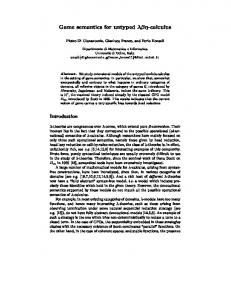
§ 0.3.12 (necessity of →red and →nil ). The purpose of →red together with →nil is to prevent unbounded growth of binding groups during unfolding. Consider for instance the outermost rewrite sequence on the term let f = let g = f g in g in f shown in fig. 0.1, where after the fourth rewriting step g ′ (the left one) becomes unreachable and could be removed by a →red -step. While restricting the size of binding groups during unfolding is a sensible constraint on the unfolding process, it is not strictly necessary to define the unfolding of a λletrec -term. Alternatively, we could employ a rule as follows: let f1 = L1 . . . fn = Ln in L →free L

(if f1 , . . . , fn do not occur in L)

Note that a →free -step can be simulated by a →red -step followed by a →nil -step. We will, however, at a later point embed the unfolding rules into other rewriting systems of which we wish to perform unfolding in a lazy way such that the number of derivable subterms is bounded. Using the →free -rule instead of →red and →nil the size of the bindings groups in fig. 0.1 keeps growing and we obtain an infinite number of different subterms. § 0.3.13 (informal notation). We will be using the informal notation as above throughout most of the thesis. For reasoning however, we lean on the theory of higher-order rewriting. In this way we can avoid the ado of an explicit substitution calculus, which would be required for sound reasoning in a firstorder formulation.


11

let f = let g = f g in g in f →rec

let f = let g = f g in g in let g ′ = f g ′ in g ′

→letrec

let

f = let g = f g in g in g ′ g′ = f g′

→rec

let

f = let g = f g in g in f g ′ g′ = f g′

→@

(let

→rec

→letrec

f = let g = f g in g f = let g = f g in g in f ) (let ′ in g ′ ) g′ = f g′ g = f g′

f = let g = f g in g in let g ′′ = f g ′′ in g ′′ ) g′ = f g′ f = let g = f g in g (let ′ in g ′ ) g = f g′

(let

f = let g = f g in g ⎞ ⎛ f = let g = f g in g in g ′ ) in g ′′ (let ′ let g ′ = f g ′ g = f g′ ⎠ ⎝ ′′ ′′ g =f g

Figure 0.1. Unbounded growth of binding groups indicated by the initial segment of an infinite →▽ -rewrite-sequence without →red -steps.

0.4

Preliminaries

Notation 0.4.1 (N, natural numbers). By N we denote the natural numbers including zero. We let N = {0, 1, . . .}. Notation 0.4.2 (functions, domain, image). For a total function f ∶ A → B we denote by dom(f ) the domain A, and by im(f ) the image B of f . For a partial function f ∶ A ⇀ B, and a ∈ A we denote by f (a)↓ that f is defined for a. The domain of f is the set dom(f ) ∶= {a ∈ A ∣ f (a)↓}. Notation 0.4.3. We denote by f ∣ D the restriction of function f to domain D. Notation 0.4.4 (rewrite relations). Let → ⊆ A × A be a rewrite relation. We denote by ↠ the many-step rewrite relation induced by →, by which we mean the reflexive and transitive closure of →. By →+ we denote the one-or-more-step rewrite relation of →, the transitive closure of →. By →= we mean the zero-orone-step rewrite relation of →, the reflexive closure of →. By →» we denote the


12

infinite rewrite relation of finitely of infinitely many →-steps (see § 1.3.25 for more details). By a normal form of → we mean an a ∈ A such that there is no a′ ∈ A with a → a′ . By →! we mean the reduction to normal form rewrite relation induced by →. It is equivalent to the restriction of ↠ to a relation with the normal forms of → as codomain: →! = {⟨a, a′ ⟩ ∣ a ↠ a′ , a′ normal form of →}.

0.5

λ-terms and λletrec -terms – CRS formalisation

§ 0.5.1 (Combinatory Reduction Systems). Many of the formalisations we introduce are based on the framework of Combinatory Reduction Systems (CRSs) [36], [37] [51, Section 11.3], and, in particular, on infinitary Combinatory Reduction Systems (iCRSs) [31]. CRSs are a higher-order term rewriting framework tailor-made for formalising and manipulating expressions in higherorder languages (i.e. languages with binding constructs like λ-abstractions and function bindings). They provide a sound basis for defining our language and for reasoning with letrec-expressions. By formalising a system of unfolding rules as a CRS we conveniently externalise issues like name capturing and α-renaming, which otherwise would have to be handled by a calculus of explicit substitution. Also, we can lean on the rewriting theory of CRSs for the proofs. Remark 0.5.2 (infinitary rewriting). We rely on CRSs (and not for instance Higher-Order Rewriting Systems (HRSs) [51]) as a rewriting framework since to date infinitary rewriting theory has only been developed for CRSs [34, 35, 31]. § 0.5.3 (the ‘calculi’ λ, λ● , and λletrec ). We will use the symbols λ, λ● , and λletrec to refer to the λ-calculus, the λ-calculus with black holes, and the λletrec calculus with letrec. However, we consider the former two calculi not to have any rewriting rules at all, since we concern ourselves only with unfolding, not with β-reduction. For formulating the rules from section 0.3 as a CRS, we provide CRS signatures for λ, λ● and λletrec . Definition 0.5.4 (CRS signatures for λ, λ● , and λletrec ). The CRS signature for λ consists of the set Σλ = {app, abs} where app is a binary (ar(app) = 2) and abs is a unary (ar(abs) = 1) function symbol. The CRS signature for λ● is Σλ● = Σλ ∪ {●} where ● is a nullary (ar(●) = 0) function symbol. The CRS signature Σλletrec consists of the countably infinite set Σλletrec = Σλ● ∪ {let} ∪ {inn ∣ n ∈ N} of function symbols, with ar(let) = 1 and ar(inn ) = n + 1 for all n ∈ N.


13

Definition 0.5.5 (set of λ-terms). By Ter∞ (λ) we denote the set of closed iCRS terms (terms in an infinitary CRS [31]) over Σλ . Likewise, we denote by Ter∞ (λ● ) the set of closed iCRS terms over Σλ● . Note that the set includes finite as well as infinite terms, thus whenever we speak of λ-terms we refer to λ-terms that are either finite or infinite. We will look more closely at iCRS-terms in § 1.3.22 Definition 0.5.6 (set of λletrec -terms). By Ter(λletrec ) we denote the set of closed CRS terms over Σλletrec , with the restrictions ○ that there is no occurrence of the ●-symbol ○ that let and inn can only occur as patterns of the form let([f1 . . . fn ] inn (. . .)) ○ and that otherwise a CRS abstraction can only occur directly beneath an abs-symbol. Example 0.5.7 (fix id). The naive version of fix applied to the identity function as in example 0.1.11 in CRS notation: app(let([fix] in1 (abs([f ] app(f, app(fix, f ))), fix)), abs([x] x)) The unfolding of fix in CRS notation: abs([f ]app(f, app(abs([f ]app(f, app(. . . , f ))), f ))) Example 0.5.8 (fix). The (not so naively implemented) fix-function from example 0.3.6 in CRS notation: abs([f ] (let([r] in1 (app(f, r), r))))

0.6

Unfolding Rules – CRS formalisation

Here we give a CRS formalisation of the rules for unfolding λletrec -terms, corresponding to unfolding as described informally in section 0.3. Definition 0.6.1 (CRSs R▽ and R▽● for unfolding λletrec -terms). R▽ and R▽● for unfolding λletrec -terms are CRSs over the signature Σλletrec . The rules of R▽● consist of all the rule schemes below, while in R▽ the last two rules schemes


14

are excluded (ϱtighten and ϱ●▽ ). We use vector notation to denote sequences ▽ ⃗ f⃗) instead of of CRS abstractions (f⃗ instead of f1 , . . . , fn ) and metaterms (B( ⃗ ⃗ B1 (f ), . . . , Bn (f )).


15

⃗ f⃗), abs([x] M (f⃗, x)))) ϱλ▽ ∶ let([f⃗] inn (B( ⃗ f⃗), M (f⃗, x)))) → abs([x] let([f⃗]inn (B( ⃗ ⃗ ⃗ ⃗ ⃗ ϱ@ ▽ ∶ let([f ] inn (B(f ), app(M (f ), N (f )))) ⃗ f⃗), M (f⃗))), let([f⃗] inn (B( → app( ⃗ ⃗ f⃗), N (f⃗))) ) let([f ] inn (B( ⃗ f⃗), let([⃗ ⃗ f⃗, g⃗), M (f⃗, g⃗))))) ϱletrec ∶ let([f⃗]inn (B( g ] inm (C( ▽ ⃗ f⃗), C( ⃗ f⃗, g⃗), M (f⃗, g⃗))) → let([f⃗g⃗] inn+m (B( ⃗ ⃗ ⃗ ⃗ ⃗ ⃗ ⃗ ϱrec ▽ ∶ let([f ]inn (B(f ), fi )) → let([f ]inn (B(f ), Bi (f ))) ϱnil ▽ ∶ let(in0 (M )) → M

, ,

⎛ ⃗ ⎛ ⎞⎞ ϱred Bi (f⃗i ) , M (f⃗′ ) ▽ ∶ let [f ]inn ⎝ ⎝i∈{1,...,n} ⎠⎠ → let([f⃗′ ] in∣I∣ (

,

Bi (f⃗′ ) , M (f⃗′ )))

i∈I

for some I ⊂ {1, . . . , n} ⎧ ′ ⎪ ⎪f⃗ with f⃗′ = fi and f⃗i = ⎨ ⃗ ⎪ f ⎪ i∈I ⎩

i∈I i ∈/ I

⃗ f⃗), M (f⃗))) where Bi (f⃗) = fj ∶ let([f⃗] inn (B( ϱtighten ▽ → let([⃗ g ] inn−1 (

B1 (⃗ g ′ ), . . . , Bi−1 (⃗ g ′ ), )) ′ Bi+1 (⃗ g ), . . . , Bn (⃗ g ′ ), M (⃗ g′ )

for some i, j ∈ {1, . . . , n} with i ≠ j and g⃗′ = ⟨g1 , . . . , gi−1 , gk , gi+1 , . . . , gn−1 ⟩ where k = j if j < i and k = j − 1 if j > i ⃗ f⃗), M (f⃗))) where Bi (f⃗) = fi ϱ●▽ ∶ let([f⃗] inn (B( → let([⃗ g ] inn−1 (

B1 (⃗ g ′ ), . . . , Bi−1 (⃗ g ′ ), )) Bi+1 (⃗ g ′ ), . . . , Bn (⃗ g ′ ), M (⃗ g′ )

for some i ∈ {1, . . . , n} and g⃗′ = ⟨g1 , . . . , gi−1 , ●, gi+1 , . . . , gn−1 ⟩


16

The first four rule schemes require little explanation. The rules are generated ⃗ and C⃗ are from having n and m range over N. The length of the vectors f⃗, g⃗, B, stipulated by the subscript of the let-symbol in accordance to definition 0.5.6. ϱnil ▽ is actually a rule, not a rule scheme. The formulation of ϱred ▽ uses, as an abbreviation, an ad-hoc list-builder notation, which works just as customary mathematical notation for, say, the union by indexing over an ordered set. Compare: ⋃ A(i) = A(i1 ) ∪ . . . ∪ A(in )

,

i∈{i1 ,...,in }

where i1 < . . . < in

A(i) = A(i1 ), . . . , A(in )

i∈{i1 ,...,in }

Moreover, in the rule scheme ϱred ▽ not only does n range over N; also the index set I ranges over all subsets of {1, . . . , n}. The purpose of the rule scheme is to remove all bindings that are not required. A binding is considered required if it is used directly or indirectly by M . I is (by formulation of the rule scheme) a superset of all required bindings, or to be more precise: for a given term, only if I is chosen as a superset of the required bindings, the rule scheme yields an CRS rule applicable to the term. From the set of ‘valid’ choices we consider the single minimal choice for I in order to remove all unrequired bindings at once. An implementation of this rule scheme would entail a reachability analysis, which is implicit here. red Example 0.6.2 (ϱred ▽ ). To understand the rule scheme ϱ▽ , consider the term L = let f1 = f2 , f2 = f1 in f1 or in CRS notation L = let([f1 f2 ] in2 (f2 , f1 , f1 )). Considering only the four possibilities we have for I, ϱred ▽ induces the following four CRS rules:

{} ∶ let([f1 f2 ] in2 (B1 (f1 , f2 ), B2 (f1 , f2 ), M ())) → let(in0 (M ())) {1} ∶ let([f1 f2 ] in2 (B1 (f1 ), B2 (f1 , f2 ), M (f1 ))) → let([f1 ] in1 (B1 (f1 ), M (f1 ))) {2} ∶ let([f1 f2 ] in2 (B1 (f1 , f2 ), B2 (f2 ), M (f2 ))) → let([f2 ] in1 (B2 (f2 ), M (f2 ))) {1, 2} ∶ let([f1 f2 ] in2 (B1 (f1 , f2 ), B2 (f1 , f2 ), M (f1 , f2 ))) → let([f1 , f2 ] in2 (B2 (f1 , f2 ), M (f1 , f2 )))


17

The first and the third rule are not applicable to L, since M has an occurrence of f1 . The rules induced by I = {1} and I = {2} are not applicable to L, because B1 has an occurrence of f2 and B2 has an occurrence of f1 . All the bindings here are used by M , therefore the only applicable rule is the last one, which does not alter L at all. Now let us consider the term L′ = let f1 = f2 , f2 = f1 in x or in CRS notation ′ L = let([f1 f2 ] in2 (f2 , f1 , x)). As before the rules induced by I = {1} and I = {2} are not applicable. However this time not only the last but also the first rule is applicable, indicating that none of the bindings are used by M and thus all of them can be removed in one →red -step. Definition 0.6.3 (garbage free). We call a λletrec -term that is a normal form nil w.r.t. to the rules ϱred ▽ and ϱ▽ garbage free. Notation 0.6.4 (ϱρ , ϱρs ). Above we used the notation ϱρs to denote a rule named ρ that belongs to the rewriting system s. We will omit the s and write ϱρ to denote a rule ρ if it is unambiguous to which rewriting system ρ belongs to. Notation 0.6.5 (rewriting relations for R▽ and R▽● ). We write →▽ (→▽● ) for the rewrite relation induced by R▽ (R▽● ). And by →λ , →@ , →letrec , →rec , →nil , →red , →tighten , and →● , we denote the rewrite relations of both the CRSs that are induced by the rules ϱλ , ϱ@ , ϱletrec , ϱrec , ϱnil , ϱred , ϱtighten , and ϱ● , respectively. Remark 0.6.6 (alternative formalisation with permutations). Note that in the rule patterns in R▽ we have to ensure that the function binding we want to refer to may be at an arbitrary position among the function bindings of a let-expression. An alternative approach would be to adding a permutation rule by which two adjacent function bindings can be swapped. Then the remaining rules which refer to a function binding could be written such that they always make use of the first function binding of the let-expression. This approach is for instance used in [17]. § 0.6.7 (informal notation). As mentioned in § 0.3.13 when studying examples we will mostly rely on the easier-to-read informal notation from section 0.3 instead of the more cumbersome CRS notation.


0.7

18

Unfolding Semantics of λletrec

Based on the CRSs R▽ and R▽● we define the unfolding semantics of λletrec terms as its infinite unique normal form. The well-definedness of the functions below is witnessed by theorem 0.7.2 below. Definition 0.7.1 (partial and total unfolding semantics). R▽ induces the unfolding semantics ⟦⋅⟧λ ∶ Ter(λletrec ) ⇀ Ter∞ (λ) L↦M

if L →»!▽ M

which is partial, because of meaningless bindings. (see § 0.3.7) R▽● induces the unfolding semantics ⟦⋅⟧λ● ∶ Ter(λletrec ) → Ter∞ (λ● ) L↦M

if L →»!▽ M ●

which is total, as it maps meaningless terms to ●. Theorem 0.7.2. ⟦⋅⟧λ and ⟦⋅⟧λ● are well-defined functions. Proof. Well-definedness of these mappings is guaranteed by the following properties of R▽ and R▽● : Lemma 0.7.6 (infinite normalisation): the existence of a normal form (only required for R▽● ) Lemma 0.7.5 (well-formedness of the normal forms): normal forms do indeed adhere to the signatures Σλ , and Σλ● , respectively. Lemma 0.7.7 (uniqueness of normal forms)

Proposition 0.7.3 (⟦⋅⟧λ is a specialisation ⟦⋅⟧λ● ). ∀L ∈ dom(⟦⋅⟧λ ) ⟦L⟧λ = ⟦L⟧λ●


19

Proof. For R▽ as well as R▽● a λletrec -term is a normal form if and only if it is a let-expression. Therefore every normal form of ⟦⋅⟧λ is a normal form of ⟦⋅⟧λ● . Reachability of the normal forms is guaranteed by the fact that the rules of R▽● are a superset of the rules of R▽ . Terminology 0.7.4. We say that a λletrec -term L unfolds to M if either ⟦L⟧λ = M or ⟦L⟧λ● = M . Which is meant, should be clear from the context. We finish the section with the lemmas required for theorem 0.7.2. Lemma 0.7.5 (well-formedness of the normal forms). R▽ (R▽● ) has λ-terms (λ● -terms) as normal forms. Proof sketch. The names of the first four rules are chosen to reflect the kind of term contained by the body of the letrec-expression, which helps to see that the rules are complete in the sense that every let-expression is a redex, thus normal forms do not contain let-expressions. Terms over Σλletrec without let-expressions are λ● -terms. The arguments also holds analogously for R▽ , which contains no rule to give rise to a ●-symbol. Lemma 0.7.6 (infinite normalisation of R▽● ). Every λletrec -term is either weakly normalising w.r.t. →▽● or admits a strongly convergent outermost-fair →▽● -rewriting-sequence. For definitions of ‘outermost fair’ and ‘strongly convergent’ we refer to [35]. Proof sketch. We consider outermost-fair →▽● -rewrite-sequences on a λletrec term L, in which ϱred , ϱnil , ϱtighten , and ϱ● are applied eagerly. We show that every such sequence τ is either finite, or that otherwise its rewrite activity tends to infinity. We argue by contradiction: We assume τ performs infinitely many rewriting steps on position p. Then there is an infinite subsequence ξ of τ which contracts only redexes at p. We show that ξ cannot exist. First note that a λletrec -term is a →▽● -redex if and only if it is a let-expression. Also an outermost →▽● -rewriting-sequence cannot create redexes upwards. Therefore, for ξ to be infinite all terms in ξ must have a let-expression at p. ξ can contain neither →λ -steps nor →@ -steps, since they would generate a function symbol at p (and thus yield a term that is not a let-expression). For the rest of the proof we argue using the concept of letrec-depth, the number of let-symbols occurring under p. ξ cannot contain an infinite number of →nil -steps because it reduces letrecdepth and no other rule increases letrec-depth.


20

Thus, ξ must have an infinite suffix π which contains no →λ -, →@ -, and →nil -steps, but only steps due to →letrec , →rec , →red , →tighten , and →● . For π to be infinite it must contain infinitely many →rec -steps since the remaining four rules are only finitely often applicable, because they manipulate or remove bindings (which can happen only once per binding), or in the case of →letrec decrease the letrec-depth. We will now go on to show that π cannot have infinitely many →rec -steps, if →tighten -steps and →● -steps take precedence. Every binding that is employed by the →rec -step can only be of the form f = g or f = let . . . in . . ., otherwise a →λ -step or a →@ -step would ensue, which we already excluded. A term with only these two forms of bindings can be reduced to a term with letrec-depth 1 with only bindings of the form f = g by applications of ϱtighten , ϱred , ϱnil , ϱrec , ϱletrec . If the bindings are cyclic, the π terminates with an application of ϱ● , otherwise the resulting term is a free variable. Lemma 0.7.7 (uniqueness of normal forms). If for a term in Ter(λletrec ) a normal form exists with respect to R▽ or R▽● , it is unique. Proof. This follows from finitary confluence (proposition 0.7.8) Proposition 0.7.8. R▽ and R▽● are confluent. Proof. Unique infinite normalisation of R▽ and R▽● follows from finitary confluence of R▽ and R▽ . In previous work [18] we proved confluence for a CRS which is very similar to R▽ . In appendix C an adapted version of that proof is provided, also extended by the rules ϱtighten and ϱ● . The proof is based on decreasing diagrams [51, Section 14.2] and involves a comprehensive critical-pair analysis. Remark 0.7.9. Note that this confluence result concerns a rewriting system only for unfolding λletrec -terms, and therefore does not conflict with nonconfluence observations concerning versions of cyclic λ-calculi which include unfolding rules as well as β-reduction [3]. § 0.7.10 (dom(⟦⋅⟧λ )). Finally we are going to characterise the domain of ⟦⋅⟧λ , thus identify those λletrec -terms that are not meaningless but unfold to some λ-term. Meaningless λletrec -terms are unproductive in the sense that during all outermost-fair R▽ -rewrite-sequences the production of symbols stagnates due to an unproductive cycle.


21

Lemma 0.7.11. Let L be a λletrec -term be a let-expression. Then exactly one of the following statements hold: ○ All maximal outermost-fair R▽ -rewriting-sequences on L solely contain let-expressions. ○ All maximal outermost-fair R▽ -rewriting-sequences on L contain finitely many let-expressions. Definition 0.7.12 (R▽ -productivity). We say that a λletrec -term L is R▽ productive if the following statement holds: ○ L does not have a →▽ -reduct that is the source of an infinite →▽ -rewritesequence consisting exclusively of outermost steps with respect to →rec , →nil , →letrec , or →red . Lemma 0.7.13. For every λletrec -terms L the following statements are equivalent: (i) L →ω ▽ M for some infinite λ-term M . (ii) L is R▽ -productive. (iii) Every maximal outermost-fair →▽ -rewrite-sequence on L is strongly convergent. Proof. (ii) ⇒ (iii), because if L is R▽ -productive then every outermost occurrence of a letrec in every →▽ -reduct will be eventually pushed down to a higher position by either a →λ -step or a →@ -step of any maximal outermostfair →▽ -sequence. Since only let-expressions are →▽ -redexes any maximal outermost-fair rewrite sequence starting from L converges to an infinite normal form. (i) follows directly from (iii). (i) ⇒ (ii) follows from lemma 0.7.11 by contradiction. If L is not R▽ -productive then it has by definition a →▽ -reduct with at least one occurrence of a letrec which cannot be pushed further down by any outermost application of any R▽ -rule. By lemma 0.7.11 the same holds for every other maximal outermost-fair rewrite sequence. Therefore L cannot unfold to a λ-term M because M may not contain any letrecs. Proposition 0.7.14 (dom(⟦⋅⟧λ )). A λletrec -term is in dom(⟦⋅⟧λ ) if and only if λ it admits no cyclic R▽ -rewriting-sequence without ϱ@ ▽ -steps and ϱ▽ -steps.


22

Proof. “⇒” follows from confluence of R▽ (proposition 0.7.8). For “⇐” we assume that L is not infinitarily normalising in R▽ . That means that any fair strategy rewrites M eventually to a reduct with root-active subterm O. The infinite rewriting sequence that only applies rules to the root of O can never λ contain any ϱ@ ▽ -steps or ϱ▽ -steps because the reduct would not be a redex. The cyclicity of this rewriting sequence follows from proposition 1.6.22. § 0.7.15 (a single-rule unfolding system in the likeness of µ-unfolding). In appendix D we present an alternative rewriting system for unfolding λletrec terms. It has only a single rule, like the canonical rewriting system for unfolding µ-terms. § 0.7.16 (outlook). Now that we have established what we mean by unfolding, we can phrase the problems we tackle in the three following chapters of this thesis: chapter 1: Here we characterise the set of λ-terms that can be expressed finitely as λletrec -terms. To this end we introduce rewriting systems for deconstructing λ-terms. These rewriting systems induce a notion of regularity on a decomposed λ-term: if the set of its components is finite it is regular. chapter 2: From the decompositions systems arise graphical representations for λ-terms in a natural way (essentially the reduction graph of a term w.r.t. a decomposition system). We study these graph representations in order to use them to reason about their respective λ-terms. chapter 3: Here we relate these graph formalisms back to λletrec and unfolding, by which we obtain concrete practical methods to analyse and manipulate λletrec -terms.

Chapter 1

Expressibility in λletrec 1.1

Overview

§ 1.1.0 (teaser). Why cannot all infinite λletrec -terms with a simple repetitive structure like λa. λb. (λa. (λb. . . . a) b) a be expressed in λletrec ? § 1.1.1 (subject matter). In this chapter we study the relationship between finite terms in λletrec and the λ-terms they express. We investigate λ-terms that are not unfoldings of any λletrec -term and we consider the question: Which are the infinite lambda terms that are λletrec -expressible in the sense that they can be obtained as infinite unfoldings of finite λletrec -terms? Or in other words: how expressive is the language λletrec ? § 1.1.2 (methods and formalisms). We introduce a rewrite system for observing λ-terms through repeated experiments carried out at the head of the term, thereby decomposing it into ‘generated subterms’. There are four sorts of decomposition steps: →λ -steps (decomposing a λ-abstraction), →@0 -steps and →@1 -steps (decomposing an application into its function and argument), and a scope-delimiting step. The scope-delimiting step comes in two variants, →del and →S , defining two rewriting systems with rewrite relations →reg and →reg+ . These rewrite relations each induce a notion of ‘λ-transition-graph’, a sort of graphical representation of λ-terms, which can be compared by means of bisimulation. We call a λ-term ‘regular’ (‘strongly regular’) if its set of →reg -reachable (→reg+ reachable) generated subterms (and therefore its λ-transition-graph) is finite. Furthermore, we analyse the binding structure of λ-terms with the concept of ‘binding–capturing chains’.

Chapter 1. Expressibility in λletrec

24

§ 1.1.3 (result). Utilising these concepts, we answer the above question by providing two characterisations of λletrec -expressibility. For all λ-terms M , the following statements are equivalent: (i): M is λletrec -expressible; (ii): M is strongly regular; (iii): M is regular, and it only has finite binding–capturing chains.

1.2

Introduction

In chapter 0 we have established how λletrec -terms serve as a finite representation of (potentially) infinite λ-terms. It is quite obvious, that not every infinite λ-term can be represented finitely, only those λ-terms come into consideration that have some kind of repetitive, or regular, structure. It turns out, however, that not even λ-terms with a regular syntax tree can always be expressed as the infinite unfolding of a term in λletrec (see example 1.2.2 below). Terminology 1.2.1 (λletrec -expressible). We say that a λ-term M is λletrec expressible if it has a representation as a (finite)1 term L in λletrec : ∃L ∈ Ter(λletrec ) M = ⟦L⟧λ We then also say that L expresses M . Note that λ-terms have infinitely many different representations as λletrec terms (see e.g. example 1.2.5 below). Example 1.2.2 (not λletrec -expressible). Consider the infinite λ-term of the form M = λa. λb. (λc. (λd. . . . c) b) a with syntax trees as shown in fig. 1.1. Even though it has a syntax tree with a regular structure, M is not λletrec -expressible. § 1.2.3 (the relevance of scopes). To understand why there is no λletrec -term that unfolds to M , it helps to consider the scopes of the abstractions in M . Informally speaking, the scope of an abstraction denotes the minimal connected portion of the term which includes the abstraction itself as well as all occurrences of the bound variable that it binds. A precise definition is given later in definition 1.7.9. The scopes of M as shown in fig. 1.1 are infinitely entangled: the scope of λa reaches into the scope of λb, the scope of λb into the scope of λc, and so on. This trait of M suggests M cannot be the result of ‘unrolling’ a λletrec -term L, since such a process would map L’s scoping structure onto M in a regular manner, and result in a term which is ‘tiled’ into finite, non-overlapping scopes with 1 Recall

that λletrec -terms are finite by definition 0.5.6.


λa

λa

λa

λb

λb

λb

@

@

@

λc

λa

a

@ λd

λb

b

@

c

a

b

λd

b

@ .. .

a

λc

a

@

@ .. .

25

.. .

@ c

Figure 1.1. Two (α-equivalent) syntax trees of M from example 1.2.2. The second syntax tree is cleary regular. The syntax tree on the right is a version of the first syntax tree with scopes depicted as box-like structures.

bounded scope-nesting depth. This excludes, intuitively, the formation of the infinite entanglement of successively overlapping scopes that can be observed in M. Example 1.2.4 (λletrec -expressible). Consider the infinite λ-term of the form M = λxy. M y x. It is λletrec -expressible as it arises as the unfolding of let f = λxy. f y x in f as witnessed by the following rewrite sequence: let f = λxy. f y x in f →rec let f = λxy. f y x in λxy. f y x →λ λx. let f = λxy. f y x in λy. f y x →λ λxy. let f = λxy. f y x in f y x →@ λxy. (let f = λxy. f y x in f y) (let f = λxy. f y x in x) →red λxy. (let f = λxy. f y x in f y) (let in x) →nil λxy. (let f = λxy. f y x in f y) x →@ λxy. (let f = λxy. f y x in f ) (let f = λxy. f y x in y) x →red λxy. (let f = λxy. f y x in f ) (let in y) x →nil λxy. (let f = λxy. f y x in f ) y x


26

λx

λx

λy

λy

@

@ x

@ y

λx

λy

@ .. .

y

λx

λy

@ x

@

x

@

y

.. .

x

@ y

Figure 1.2. Syntax tree of M from example 1.2.4, and a version annotated with scopes. →rec . . . As shown in fig. 1.2 the syntax tree of M has some entanglement (the scopes of λx and λy do overlap) but the entanglement is finite as opposed to the entanglement in example 1.2.2. Example 1.2.5 (λletrec -expressible). The infinite λ-term λf. f (f (f . . .)) from example 0.3.6 can be expressed by L as well as by P defined as follows: L ∶= λf. let r = f r in r

P ∶= λf. let r = f (f r) in r

It holds that ⟦L⟧λ = λf. f (f (f . . .)) = ⟦P ⟧λ . See fig. 1.3 for the corresponding ‘syntax graphs’. There is only one abstraction, so trivially there are no overlapping scopes. § 1.2.6 (regularity of first-order terms). Over a first order signature, the simplest kind of infinite terms are those that are regular in the sense that they possess only a finite number of different subterms. They correspond to trees


27

λf @ f

@ f

@ f

λf. let r = f r in r →»▽

.. .

λf. f (f (f . . .))

«←▽ λf. let r = f (f r) in r

Figure 1.3. The ‘syntax graphs’ of the λletrec -terms from example 1.2.5 and the syntax tree of their unfolding.

over ranked alphabets that are regular [13]. Like regular trees, also regular terms can be expressed finitely by systems of recursion equations [13] or by ‘rational expressions’ [13, Definition4.5.3], which correspond to µ-terms (see e.g. [15]). Hereby finite expressions denote infinite terms either via a mathematical definition (a fixed-point construction, or induction on paths) or as the limit of a rewrite sequence consisting of unfolding steps. § 1.2.7 (regularity of higher-order terms). For higher-order terms such as λ-terms the concept of regularity is less clear-cut from the outset, due to the presence of variable bindings. Frequently, regularity has been used to denote the existence of a first-order representation with named variables that is regular (e.g. in [3, 1]). According to that definition M from example 1.2.2 would be regular: while the syntax tree on the left in fig. 1.1 of the term M contains infinitely many variables (and therefore is not regular), M has another α-equivalent regular syntax tree (on the right) that uses only two variable names. However, such a definition of regularity has two drawbacks: it does not (as desired) correspond to λletrec -expressibility; and it relies on a property of a first-order representation. We will attempt to find a stronger, more direct definition of regularity for λ-terms that arises as an adaptation of the first-order notion of regularity. § 1.2.8 (subterms of higher-order terms). The first-order notion of regularity relies on the finiteness of the number of subterms. When adapting this notion to higher-order terms, the problem is that there is no immediate, self-evident


28

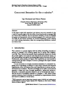
notion of subterm. Should for instance y be considered a subterm of λx. x which is after all equivalent to λy. y? In order to arrive at a viable notion of higher-order subterms we define a CRS for decomposing higher-order terms. The decomposition ‘remembers’ the abstractions encountered and ‘saves’ them as part of the such obtained components which we call ‘generated subterms’. § 1.2.9 (prefixed subterms). Viable notions of subterms for λ-terms in a higherorder formalisation require a stipulation on how to treat variable binding when descending into the body of a λ-abstraction. For this purpose we enrich the syntax of λ-terms with a parenthesised prefix of abstractions (similar to a proof system for weak µ-equality in [15, Figure 12]). An expression (λx1 . . . xn ) M represents a partially decomposed λ-term: the body M typically contains free occurrences of variables which in the original λ-term were bound by λabstractions that have been split off by decomposition steps. The role of such abstractions has then been taken over by abstractions in the prefix (λx1 . . . xn ). In this way expressions with abstraction prefixes can be kept closed under decomposition steps. § 1.2.10 (decomposition CRSs). On these prefixed λ-terms, we will define two closely related rewrite systems Reg and Reg+ . Rewrite sequences in Reg and in Reg+ deconstruct λ-terms by steps that typically decompose applications and λ-abstractions that occur just below the abstraction prefix. Reg and Reg+ differ with respect to the steps for removing vacuous prefix bindings they facilitate: while such bindings can always be removed by pertinent steps in Reg, the system Reg+ only enables steps that remove vacuous bindings at the end of the abstraction prefix. § 1.2.11 (scope-delimiting strategies). For each of these systems we consider a family of strategies that make deterministic choices concerning the application of the steps for removing vacuous prefix bindings: we call these strategies ‘scope-delimiting strategies’ for Reg, and ‘scope+ -delimiting strategies’2 for Reg+ . Scope-delimiting strategies S for Reg and scope+ -delimiting strategies S+ for Reg+ induce rewrite relations →S and →S+ , respectively. These families of rewrite strategies define respective notions of ‘generated subterm’, and they give rise to differently strong concepts of regularity: a λ-term M is called regular (strongly regular) if there is a rewrite strategy S for Reg (a rewrite strategy S+ for Reg+ ) such that the set of from M →S -reachable (→S+ -reachable) generated subterms is finite. 2 We

usually say ‘extended scope’ when pronouncing scope+ , see § 1.4.5


λx

λx

λy

λy

@

@ x

@

λy

@

@ x

.. .

y

syntax tree

λy x

λy @ x

@

x

.. .

scopes

scope+

y

()T

λy

λ (λx) λy.T y x x

y

λ (λxy) T y x

S

@0

y

λx

y

@ .. .

λx

@

λy @

y

@

@

λx

x

@

binding–capturing chains

λx

@

y

λx

λy @

x

@

y

λx

.. .

29

@1

(λxy) T y

(λxy) x

@0 @1

S

(λxy) T

(λxy) y (λx) x

S

(λx) T

→S+eag -generated subterms

Figure 1.4. Various depictions of the strongly regular infinite λ-term that is expressed by the λletrec -term let f = λxy. f y x in f .


30

Example 1.2.12 (Reg+ -decomposition). Before giving definitions of the decomposition CRSs (introduced in section 1.4) let us consider an example and decompose3 the λ-term M of the form M = λxy. M y x from example 1.2.4. The set of generated subterms consists of these prefixed terms (in no particular order): () M (λx) λy. M y x (λxy) M y x (λxy) M y (λxy) M (λx) M (λxy) y (λxy) x (λx) x. Here, (λxy) M y for instance is a witness for M y being a (generated) subterm of M , with the variables x and y being bound ‘somewhere above’. We could of course also have written (λxz) M z, which is equivalent. So why is the subterm (λxy) x in the list along with (λx) x, if x occurs at a position where both x and y have been bound? It is, because the decomposition rewrite systems include rules to remove variables from the prefix when no longer required (for leaving the scope). See fig. 1.4 for the reduction graph (Terminology 1.3.10) of M , which illustrates how the decomposition deconstructs M into the generated subterms above. Since () M has only 9 different →S+eag -reducts, the term M is strongly regular. § 1.2.13 (result). The generalisations of the concept of regularity to λ-terms suggest the question: do the expressibility results in [13] for regular first-order trees with respect to systems of recursion equations, rational expressions, or µ-terms also generalise in an appropriate way? We tackle only the case of strong regularity here, and obtain an expressibility result with respect to the λletrec , the λ-calculus with letrec. We show that an infinite unfolding is unique if it exists, and it can be obtained as the limit of an infinite rewrite sequence of unfolding steps. We prove that a λ-term is λletrec -expressible if and only if it is strongly regular. This result confirms a conjecture4 by Blom in [8, Section 1.2.4]. § 1.2.14 (chapter overview). section 1.3 introduces formalisms used in this chapter, predominantly concerning abstract rewriting systems and rewriting strategies. In section 1.4 we introduce rewriting systems for decomposing λterms into ‘generated subterms’, and we show some properties of these systems 3 The term is decomposed with respect to the ‘eager scope-delimiting’ strategy S+ eag for Reg+ ; see definition 1.4.34. 4 Cf. the last sentence of [8, Section 1.2.4]: ‘We conjecture that the set of regular lambdatrees is precisely the set of lambda-trees that can be obtained as the unwinding of terms with letrec’. Mind that ‘regular lambda-trees’ there correspond to strongly regular λ-terms in our sense, and that the notion of ‘sub-tree’ of a ‘lambda-tree’ corresponds to our notion of →S+ -generated subterm with respect to a scope+ -delimiting strategy S+ for Reg+ .


31

in connection to so-called scope-delimiting strategies. Also in this section, we define regularity and strong regularity for λ-terms employing the concepts of generated subterms and scope-delimiting strategies. In section 1.5 we adapt the rewrite systems for decomposing λ-terms and the notions of scope-delimiting strategies to the λ-calculus with letrec. In section 1.6, we develop proof systems for the notions of regularity and strong regularity, for equality of strongly regular λ-terms, and for the property of a λletrec -term to unfold to a λ-term. In section 1.7 we examine the binding structure of λ-terms (binding–capturing chains) and connect to the concepts introduced so far. In section 1.8 we establish the correspondence between strong regularity and λletrec -expressibility for λ-terms. In section 1.9 we introduce ‘λ-transition-graphs’ of λ-terms and of λletrec -terms as labelled transition graphs in which the edges carry one of the four different labels @0 , @1 , λ, and S. Section 1.10 summarises the above results.

1.3

Preliminaries

This section gathers known concepts vital to this chapter. Some notions concerning rewriting are recapitulated from [51], for others references are given. Some definitions of known concepts are simplified or tailored to our purposes. Notation 1.3.1 (∣w∣, length of a word w). For words w over some alphabet we denote the length of w by ∣w∣. We will use the following specific version of K˝onig’s Lemma. § 1.3.2 (K˝onig’s Lemma). Let G = ⟨V, E⟩ be an undirected graph with set V of vertices and set E of edges. Suppose that G has infinitely many vertices (V is infinite), that it is connected (for all vertices v, w ∈ V there exists a path in G from v to w) and that every vertex has finite degree (it is adjacent to only finitely many other vertices in G). Then for every vertex v ∈ V , G contains an infinitely long simple path from v, that is, a path starting at v without repetition of vertices.5 5 This formulation corresponds to the following original formulation by D´ enes K˝ onig [38, page 80] “Satz 3: Jeder unendliche zusammenh¨ angende Graph G endlichen Grades besitzt einen einseitig unendlichen Weg, wobei der Anfangspunkt P0 dieses Weges beliebig vorgeschrieben werden kann.” in connection with the definition [38, page 10 ] “Eine unendliche Menge von Kanten Pi Pi+1 (i = 0, 1, . . . in inf.), bzw. der durch sie gebildete Graph, heißt ein einseitig unendlicher Weg, falls f¨ ur i ≠ j stets Pi ≠ Pj ist.”


32

Rewriting Relations Notation 1.3.3 (R ⋅ S, composition of relations R and S). For relations R ⊆ A × B and S ⊆ B × C we denote by R ⋅ S the composition of R with S defined by R ⋅ S ∶= {⟨x, z⟩ ∣ (∃y ∈ B)⟨x, y⟩ ∈ R ∧ ⟨y, z⟩ ∈ S} ⊆ A × C. Notation 1.3.4 (R∗ , reflexive transitive closure of a relation R). For a relation R ⊆ A×B we denote by R∗ the reflexive transitive closure of R under composition, for which it holds that R∗ ∶= ⋃i∈N Ri where R0 ∶= idA ∶= {⟨x, x⟩ ∣ x ∈ A} and, for all i ∈ N, Ri+1 ∶= R ⋅ Ri .

Abstract Rewriting Systems We use abstract rewriting systems (ARSs) to reason about CRSs (from which we derive the ARSs) and more specifically about the set of terms that a term can be reduced to in an arbitrary number of reductions. ARSs are essentially binary relations on sets. They are in a sense graph-like structures, and more tangible in comparison to CRSs and therefore easier to manipulate. § 1.3.5 (abstract rewriting systems). An abstract rewriting system (ARS) is a quadruple ⟨O, Φ, src, tgt⟩ consisting of a set O of objects, a set Φ of steps, and src, tgt ∶ Φ → O, the source and target functions. For objects o ∈ O we denote by Φout (o) and by Φin (o) the set of steps in Φ that depart (are outgoing steps) from o, and that arrive (are incoming steps) at o, respectively. We say that an ARS is finite if Φ is finite. § 1.3.6 (ARS induced by a CRS/iCRS). Let C be a CRS/iCRS over signature Σ with rules R and let Ter(Σ)/Ter∞ (Σ) be the set of terms over Σ. We call the ARS A = ⟨O, Φ, src, tgt⟩ the ARS induced by C where: O = Ter(Σ) / O = Ter∞ (Σ) Φ = {⟨s, ρ, t⟩ ∣ s, t ∈ O, ρ ∈ R, s →ρ t} src ∶ ⟨s, ρ, t⟩ ↦ s tgt ∶ ⟨s, ρ, t⟩ ↦ t Notation 1.3.7 (induced ARS steps). While the ARS formalism makes no qualitative distinction between different kinds of steps (Φ being an unstructured set in the definition of ARS), in § 1.3.6 we retain the original information from the CRS C as to which rule a step stems from (Φ being a set of triples). This allows us to do more fine-grained reasoning and we will continue to write


33

o1 →ρ o2 to indicate that there is a step φ ∈ Φ with src(φ) = o1 and tgt(φ) = o2 which is due to the application of a CRS rule ϱρC , or even o1 →A.ρ o2 to indicate which ARS we mean specifically. We sometimes also name the step specifically and write φ ∶ o1 →ρ o2 or φ ∶ o1 →A.ρ o2 . § 1.3.8 (sub-ARS). Let A1 = ⟨O1 , Φ1 , src1 , tgt1 ⟩ and A2 = ⟨O2 , Φ2 , src2 , tgt2 ⟩ be ARSs. We say that A1 is a sub-ARS of A2 if O1 ⊆ O2 , Φ1 ⊆ Φ2 , and src1 , tgt1 are the restrictions of src2 and tgt2 , respectively, to Φ1 , which are required to be total functions. This implies that, for all φ ∈ Φ1 , it holds that src2 (φ) = src1 (φ) ∈ O1 , and tgt2 (φ) = tgt1 (φ) ∈ O1 . § 1.3.9 (generated sub-ARS). For an object o ∈ O of an ARS A = ⟨O, Φ, src, tgt⟩ we denote by (o ↠) ∶= ⟨O′ , Φ′ , src′ , tgt′ ⟩ the sub-ARS of A generated by o, where O′ comprises only the objects from O that are reachable from o by an arbitrary number of steps (or no steps) and with Φ′ , src′ , tgt′ being the restrictions of Φ, src, tgt to the objects in O′ and to steps between objects in O′ . We write (o ↠A ) to explicitly refer to a specific ARS. Terminology 1.3.10 (reduction graph). We call (o ↠) the reduction graph of o, and (o ↠A ) the reduction graph of o with respect to A.

ARS Strategies Next we will give definitions for history-free and history-aware strategies for ARSs. The latter is based on the notion of ARS labelling which in turn is based on the notion of ARS bisimulations. Note that ARS bisimulation is solely introduced for the sake of defining ARS labellings and is not to be confused with bisimulation between LTSs or TRSs. § 1.3.11 (bisimulation between ARSs). Let Ai = ⟨Oi , Φi , srci , tgti ⟩ for i ∈ {1, 2} be ARSs. A relation B ⊆ (O1 × O2 ) ∪ (Φ1 × Φ2 ), which relates objects with objects and steps with steps, is called an ARS bisimulation between A1 and A2 if the following holds: ○ if B relates two objects, then B also relates their outgoing steps: ∀⟨o1 , o2 ⟩ ∈ O1 × O2 o1 B o2 ⇒ ∀φ1 ∈ Φ1out (o1 ) ∃φ2 ∈ Φ2out (o2 ) φ1 B φ2 ∧ ∀φ2 ∈ Φ2out (o2 ) ∃φ1 ∈ Φ1out (o1 ) φ2 B φ1


34

○ if B relates two steps, then B also relates their sources and targets: ∀⟨φ1 , φ2 ⟩ ∈ Φ1 × Φ2 φ1 B φ2 ⇒ src1 (φ1 ) B src2 (φ2 ) ∧ tgt1 (φ1 ) B tgt2 (φ2 ) In this work we need ARS-bisimulation only to define ARS-labellings: § 1.3.12 (labellings of ARSs). Let A = ⟨O, Φ, src, tgt⟩ and A′ = ⟨O′ , Φ′ , src′ , tgt′ ⟩ be ARSs. (i) An ARS bisimulation L between A and A′ is called a labelling of A to A′ , and A′ the L-labelled version of A, if the converse L⌣ of L is a function L⌣ ∶ O′ ∪ Φ′ → O ∪ Φ, and if additionally, for all o′ ∈ O′ and o ∈ O with o L o′ , the restriction L⌣ ∣ Φ′out (o′ ) ∶ Φ′out (o′ ) → Φout (o) of L⌣ to the steps departing from o′ is bijective. (ii) A rewrite labelling L of A to A′ is a pair ⟨L, l⟩ consisting of a labelling L of A to A′ together with an initial labelling function l mapping objects of A to bisimilar objects of A′ . § 1.3.13 (history-free strategy). A history-free strategy for an abstract rewriting system A is a sub-ARS of A that has the same objects, and the same normal forms as A. § 1.3.14 (history-aware strategy). A history-aware strategy for an abstract rewriting system A is a history-free strategy for the L-labelled version of A with respect to, and together with, a rewrite labelling ⟨L, l⟩ of A. § 1.3.15 (history-aware and history-free strategies). While strategies are simply defined as sub-ARSs of an ARS, here one may think of them as restrictions on the applicability of CRS rules. This is because in this work we consider ARSs that are induced by a CRS. A history-free strategy cannot restrict the applicability of a CRS rule to some term differently depending on the history (i.e. the previously applied rules) of that term. In history-aware strategy, on the other hands, terms are coupled with additional information that can be used to record the history of a term. Thus, how the applicability of CRS rules are restricted can differ depending on that record. By a strategy for A we will mean a history-free strategy or a history-aware strategy for A.


35

§ 1.3.16 (projecting history-aware strategies to history-free strategies). Let S be a history-aware strategy for A, and let A′ be that L-labelled version of A which S is a history-free strategy for. Then S projects to a history-free ˇ of A. The projection is defined by L, which induces a local bijective strategy S correspondence between outgoing steps of related sources of A and A′ . Mind ˇ may become non-deterministic. Furthermore, every that for deterministic S, S rewrite sequence according to S in A′ projects to a unique rewrite sequence in ˇ A (which is a rewrite sequence according to S). The last mentioned fact makes it possible to speak, for a given rewrite labelling, of rewrite sequences of a history-aware strategy for the objects of the original ARS. Let S be a history-aware strategy for an ARS A, and o an object of A. Suppose that S is a sub-ARS of the L-labelled version A′ of A for some rewrite labelling ⟨L, l⟩ of A. Then by a rewrite sequence of S on o (in A) we will mean the projection to A of a rewrite sequence of S (in A′ ) on the result l(o) of the initial labelling applied to o.

Labelled Transition Systems § 1.3.17 (labelled transition systems). A labelled transition system (LTS) is a triple L = ⟨S, L, T ⟩ consisting of a set S of states, a set L of labels, and a set T ⊆ S × L × S of L-labelled transitions. We write s1 →a s2 to denote labelled transitions, indicating that ⟨s1 , a, s2 ⟩ ∈ T . § 1.3.18 (bisimulation between LTSs). Let L1 = ⟨S1 , L, T1 ⟩ and L2 = ⟨S2 , L, T2 ⟩ be a LTSs over a common set of labels. A bisimulation on L is a binary relation R ⊆ S1 × S2 that satisfies, for all s1 ∈ S1 and s2 ∈ S2 : (i) if s1 R s2 and s1 →a s′1 , then there exists s′2 ∈ S2 such that s2 →a s′2 and s′1 R s′2 ; (ii) if s1 R s2 and s2 →a s′2 , then there exists s′1 ∈ S1 such that s1 →a s′1 and s′1 R s′2 . Two states s1 ∈ S1 and s2 ∈ S2 are bisimilar, denoted by s1 ↔ s2 , if there exists a bisimulation R such that s1 R s2 . Remark 1.3.19 (ARSs versus LTSs). Note that labelled transition systems (LTSs) are essentially the same as (indexed) ARSs [51, 1.1]. Traditionally, research about LTSs is more concerned with the transitions and their labels


36

while research about ARSs is more concerned with set of objects and their reachability. This is reflected in a different definition of bisimulation for the two systems. Only on LTSs the bisimulation is sensitive to transition labels; ARSs do not have explicit labels on their steps. In this work we adhere to the tradition. We use ARSs for the definition of (strong) regularity which depends on whether the set of reachable terms is finite, and we use LTSs to define a graph representation for λ-terms on which we study properties revolving around (functional) bisimulation. § 1.3.20 (labelled transition graphs). A labelled transition graph (LTG) G is a pointed LTS, that is, G = ⟨S, L, i, T ⟩ where ⟨S, L, T ⟩ is an LTS, and i ∈ S, which is called the initial state. § 1.3.21 (bisimulation between LTGs). Two LTGs G1 = ⟨S1 , L, i1 , →1 ⟩ and G1 = ⟨S2 , L, i2 , →2 ⟩ are bisimilar if there is a bisimulation on the underlying LTSs that relates the initial states i1 and i2 with one another.

iCRS Terms § 1.3.22 (iCRS preterms, iCRS terms). When speaking of ‘infinite terms’ for CRSs over some signature we draw on [51, 12.4] and [31] where metaterms of iCRSs are defined by means of metric completion. The metric is defined on α-equivalence classes of finite metaterms dependent on the minimal depth at which two finite preterms belonging to the equivalence classes have a ‘conflict’. iCRS terms are defined as the objects formed by the metric completion process. They can be represented as equivalence classes of infinite preterms, which we call iCRS preterms, with respect to a notion of α-equivalence that again is based on the notion of ‘conflict’ (see also [51, Definition 12.4.1]). iCRS preterms are infinite ordered dyadic trees in which each node is either labelled by a variable name, and then the node does not have a successor, or by named abstractions λx (with some variable name x), and then the node has a single successor node, or by an application symbol, and then the node has a right and a left successor node. Definition 1.3.23 (α-equivalence for iCRS preterms, Schroer-style proof system). The notion of α-equivalence on iCRS preterms based on the absence of conflicts can be described by provability in the proof system A∞ S (Σ) in fig. 1.5 which is an adaptation of a proof system due to Schroer [26]. The proof system A∞ S (Σ) over signature Σ consists of the axioms and rules displayed in fig. 1.5 and contains a rule f for every f ∈ Σ. Provability in A∞ S (Σ) of an equation


c = c const

37

s[x ∶= c] = t[y ∶= c] [] [x]s = [y] t

s1 = t1 ...... sn = tn f f (s1 , . . . , sn ) = f (t1 , . . . , tn ) Figure 1.5. Schroer-style proof system A∞ S (Σ) for α-equivalence of iCRS preterms over signature Σ: for every f ∈ Σ with arity n, A∞ S (Σ) contains a rule f . In instances of the rule [ ], the constant c is chosen fresh for s and t. Substitution which occurs in the assumption of [ ] denotes substitution by variable replacement on iCRS preterms. It needs not to be capture-avoiding because of the freshness of the substituant.

between preterms is defined as the existence of a possibly infinite, completed derivation: for example, by ∞ ⊢A∞S s = t we mean the existence of a possibly infinite proof tree D∞ with conclusion s = t such that maximal threads from the conclusion upwards either have length ω, or have finite length and end at a leaf that carries an axiom. (We will generally use the decorated turnstyle symbol ∞ ⊢ to indicate provability by a completed, possibly infinite derivation.) However, closer to coinductive proof systems for λ-terms that we develop is the following different, but equivalent characterisation of α-equivalence for infinite iCRS preterms, a variant for iCRS terms of a proof system for αequivalence between finite λ-terms due to Kahrs (see [26]). Definition 1.3.24 (α-equivalence for iCRS preterms, Kahrs-style proof system). The proof system A∞ K (Σ) for α-equivalence on iCRS preterms over signature Σ consists of the axioms and the rules in fig. 1.6 with, for every f ∈ Σ, a rule f . Provability of an equation between preterms in A∞ K (Σ) is defined, analogously as in fig. 1.5, as the existence of a possibly infinite, completed derivation. This formulation of α-equivalence for λ-terms will be the key to our formulation of a ‘coinduction principle’ for λ-terms in theorem 1.9.12. § 1.3.25 (infinite rewrite relation, →»). For an iCRS with rewrite relation →, we denote by →» the infinite rewrite relation induced by strongly convergent and continuous rewrite sequences of arbitrary (countable) ordinal length. Hereby strong convergence means that, at every limit ordinal, the depth of the rewrite


{⃗ xy}y = {⃗ z u} u

38

0

{⃗ x} s = {⃗ z }t (if y does not occur in s, S and w does not occur in t) {⃗ xy}s = {⃗ z w}t {⃗ xy} s = {⃗ z u}t [] {⃗ x} [y] s = {⃗ z } [u]t {⃗ x} s1 = {⃗ y }t1 ...... {⃗ x} sn = {⃗ y } tn f {⃗ x}f (s1 , . . . , sn ) = {⃗ y }f (t1 , . . . , tn ) Figure 1.6. Kahrs-style proof system A∞ K (Σ) for α-equivalence on iCRS preterms over signature Σ: for every f ∈ Σ with arity n, A∞ K (Σ) contains a rule f.

activity in the rewrite sequence’s terms tends to infinity. Continuity means that the terms of the rewrite sequence converge, in the metric space of infinite terms, at every limit ordinal. By →ω we will denote the rewrite relation induced by strongly continuous →-rewrite-sequences of length ω.

1.4

Regular and strongly regular λ-terms

§ 1.4.1 (regularity). For infinite first-order trees the concept of regularity is well-known and well-studied [13]. Regularity of a labelled tree6 is defined as the existence of only finitely many subtrees and implies the existence of a finite graph that unfolds to that tree. In this section we generalise the notion of regularity to trees with a binding mechanism, i.e. to λ-terms specifically. We give a definition for regularity which corresponds to regularity of a term when regarded as a first-order tree, and for strong regularity, which will be shown in the following sections to coincide with λletrec -expressibility. 6 By a ‘labelled tree’ we here mean a finite or infinite tree whose nodes are labelled by function symbols with a fixed arity. The arity determines the number of (ordered) successor nodes each node has.


39

§ 1.4.2 (decomposition CRSs Reg and Reg+ ). We define regularity and strong regularity in terms of rewriting systems that will be called Reg and Reg+ . Rewrite sequences in these systems inspect a given term coinductively in the sense that a rewrite sequence corresponds to a decomposition of the term along one of its paths from the root. Both Reg and Reg+ extend a kernel system Reg− comprising three rewrite rules which denote whether the position just passed in the tree is an abstraction or an application and in the second case whether the application is being followed to the left or to the right. § 1.4.3 (prefixed terms). The rewriting systems are defined on λ-terms enriched by what we call an abstraction prefix, by which the terms can be kept closed during the deconstruction. This is crucial for the definition of the rewriting system as a CRS. While intuitively it is clear that the λ-term M N is composed of the subterms M and N , abstractions are more problematic. In a first-order setting one could say that λx. M contains M as a subterm, but if x occurs freely in M then M would be an open term. That means that the scrutinisation of an abstraction would be able to go from a closed term to an open term, which would run counter to the interpretation of a higher-order term as an α-equivalence class. In the definition of the rewriting systems below this issue is resolved as follows. When inspecting an abstraction, the binder is eliminated but moved from the scrutinised subterm into the prefix. That guarantees that the term as a whole remains closed. Example 1.4.4. In λx. λy. x x y for instance the path from the root to the second occurrence of x then corresponds to the rewrite sequence: () λx. λy. x x y →λ (λx) λy. x x y →λ (λxy) x x y →@0 (λxy) x x →@1 (λxy) x. § 1.4.5 (scope and scope+ ). The Reg and the Reg+ system extend Reg− by a scope-delimiting rule, which signifies that the scope of an abstraction has ended, with both systems being based on different notions of scope. Reg relies on what we simply call scope of an abstraction: the range from the abstraction up to the positions under which the bound variable does not occur anymore. We base Reg+ on a different notion of scope, called scope+ (pronounced ‘extended scope’), which is strictly nested. The scopes+ of an abstraction extends its scope by encompassing all scopes+ that are opened within its range. As a consequence, scopes+ do no overlap partially (see fig. 1.7) but are strictly nested. In a sense scope+ is the transitive closure of scope; this becomes obvious in definition 1.7.9 where a precise definition of scope and scope+ is given. In [5] scopes+ are called ‘skeletons’.


λx

λx

λy

λy

@

@ y

@ x

40

x

y

@ x

x

Figure 1.7. The difference between scope and scope+ § 1.4.6 (scope+ -delimiters identify abstractions). When every scope+ is closed by the scope+ -delimiting rule then the sequence of rewrite steps alone (i.e. without the terms themselves) unambiguously determines which abstraction a variable occurrence belongs to. Example 1.4.7. The rewrite sequence from above would then have one additional scope+ -delimiting step asserting that the variable at the end of the path is indeed x and not y: () λx. λy. x x y →λ (λx) λy. x x y →λ (λxy) x x y →@0 (λxy) x x →@1 (λxy) x →S (λx) x § 1.4.8 (abstraction prefix and scope+ ). The abstraction prefix not only keeps the term closed but also denotes which scope+ is still open, which provides the information to decide applicability of the scope+ -delimiting rule. Example 1.4.9. The last step closes the scope+ of y, therefore that variable is removed from the prefix. The rewrite sequence for the path to the occurrence of y does not include a scope+ -delimiting step: () λx. λy. x x y →λ (λx) λy. x x y →λ (λxy) x x y →@1 (λxy) y § 1.4.10 (nameless representation for λ-terms). Ultimately, the Reg+ rewriting system defines nameless representations for λ-terms related to the de-Bruijn notation for λ-terms. Considering the de-Bruijn representation of the above term λ. λ. S(0) S(0) 0 we find that the position of the →S -steps indeed coincides with the position of the S markers. However, the rewrite system Reg+ permits more flexibility for the placement of →S -steps. Example 1.4.11. For example the path from example 1.4.7 to the second occurrence of x can also be witnessed by the following rewrite sequence: () λx. λy. x x y →λ (λx) λy. x x y →λ (λxy) x x y →@0 (λxy) x x →S


41

(λx) x x →@1 (λx) x. Here the scope+ of y is closed earlier. This would correspond to λ. λ. S(0 0) 0 in de-Bruijn notation, or more precisely, in a variant of the de-Bruijn notation which permits the scope/scope+ -delimiter S to occur anywhere between a variable occurrence and its binding abstraction. § 1.4.12 (scope delimiters in the literature). This variation of the de-Bruijn notation [10], in which S-symbols can be used anywhere in the term signify the end of a scope, is due to Paterson [7]. The idea is also used in [47] and related to an even more flexible end-of-scope symbol λ [26]. Definition 1.4.13 (CRS terms with abstraction prefixes). The CRS signature for (λ), the λ-calculus with abstraction prefixes, extends the CRS signature Σλ for λ (see definition 0.5.4) and consists of the set Σ(λ) = Σλ ∪ {pren ∣ n ∈ N} of function symbols, where for n ∈ N the function symbols pren for prefix λabstractions of length n are unary (have arity one). CRS terms with leading prefixes pren ([x1 ]. . . [xn ]M ) will informally be denoted by (λx1 . . . xn ) M , abbreviated as (λ⃗ x) M . Definition 1.4.14 (the CRSs Reg− , Reg, Reg+ for decomposing λ-terms). Consider the following CRS rule schemes over Σ(λ) : 0 ϱ@ x), Z1 (⃗ x))) → pren ([x1 . . . xn ]Z0 (⃗ x)) ∆ ∶ pren ([x1 . . . xn ] app(Z0 (⃗ 1 ϱ@ x), Z1 (⃗ x))) → pren ([x1 . . . xn ]Z1 (⃗ x)) ∆ ∶ pren ([x1 . . . xn ] app(Z0 (⃗

ϱλ∆ ∶ pren ([x1 . . . xn ] abs([xn+1 ] Z(⃗ x))) → pren+1 ([x1 . . . xn+1 ]Z(⃗ x)) ϱS∆ ∶ pren+1 ([x1 . . . xn+1 ]Z(x1 , . . . , xn )) → pren ([x1 . . . xn ] Z(x1 , . . . , xn )) ϱdel ∆ ∶ pren+1 ([x1 . . . xn+1 ]Z(x1 , . . . , xi−1 , xi+1 , . . . , xn+1 )) → pren ([x1 . . . xi−1 xi+1 . . . xn ]Z(x1 , . . . , xi−1 , xi+1 , . . . , xn+1 )) + @1 λ 0 By Reg− we denote the CRS with rules ϱ@ ∆ , ϱ∆ , and ϱ∆ . By Reg (by Reg ) we S denote the CRS consisting of all of the above rules except the rule ϱ∆ (except the − + rule ϱdel ∆ ). The rewrite relations of Reg , Reg, and Reg are denoted by →reg− , →reg and →reg+ , respectively. And by →@0 , →@1 , →λ , →S , →del , we respectively @1 λ 0 denote the rewrite relations induced by each of the single rules ϱ@ ∆ , ϱ∆ , ϱ∆ , S del ϱ∆ , and ϱ∆ .

§ 1.4.15 (Reg− , Reg, and Reg+ in informal notation). For better readability we will from now on rely on the informal notation corresponding to definition 1.4.14


42

which is as follows: 0 ϱ@ ∆

∶ (λx1 . . . xn ) M0 M1 → (λx1 . . . xn ) M0

1 ϱ@ ∆ ϱλ∆ ϱS∆

∶ (λx1 . . . xn ) M0 M1 → (λx1 . . . xn ) M1 ∶ (λx1 . . . xn ) λxn+1 . M0 → (λx1 . . . xn+1 ) M0 ∶ (λx1 . . . xn+1 ) M0 → (λx1 . . . xn ) M0 (if the binding λxn+1 is vacuous)

ϱdel ∆

∶ (λx1 . . . xn+1 ) M0 → (λx1 . . . xi−1 xi+1 . . . xn+1 ) M0 (if the binding λxi is vacuous)

Remark 1.4.16. Be reminded that as mentioned in Notation 0.6.4 we will at times omit the ∆ and write ϱρ instead of ϱρ∆ . § 1.4.17 (Reg+ defines nameless representations). Considering the reduction graphs from fig. 1.8 without labels on their nodes we see that only from the Reg+ graph the original term can be reconstructed unambiguously. For example, the path to the rightmost occurrence of x has the rewrite sequence in Reg →λ . →λ . →@0 . →del . →@1 which witnesses an occurrence of y in place of x at the same position. This ambiguity plays a role for the definition of λ-transition-graphs in section 1.9, and is discussed in that context in § 1.9.14. § 1.4.18 (→reg+ ⊆ →reg ⊆ →reg− ). Note that →reg is contained in →reg− , and since the rule ϱdel generalises the rule ϱS , →reg+ is contained in →reg . We will specifically need the following statement later on: Proposition 1.4.19. Every rewrite sequence in Reg+ corresponds directly to a rewrite sequence in Reg by exchanging →S -steps with →del -steps. § 1.4.20 (abstract prefix symbol). We are only interested in terms which have a single occurrence of the abstraction prefix symbol at the outermost position. Note that the rules in Reg and Reg+ guarantee that every reduct of a term of the form (λ⃗ x) M is again a term of this form. Therefore we define:


λ

λ

λ

x

x

x

λ

λ

λ

xy

xy

xy

@0 @1 xy

@0 @1 xy

43

xy

del @0 @1

xy

xy

@0 @1 del

x

@0 @1

@0 @1

xy

xy

y

del

S

(M ↠Reg )

@0 @1

x

xy

@0 @1

x

(M ↠Reg− )

xy

S

x

(M ↠Reg+ )

Figure 1.8. The reduction graphs of M = () λx. λy. x x y with respect to Reg− /Reg/Reg+ . Note, that in the vertices not the entire (λ)-terms are displayed but only the respective prefixes. Definition 1.4.21 (prefixed λ-terms). By Ter∞ ((λ)) we denote the subset of closed iCRS terms over Σ(λ) with the restrictions: ○ Every term M ∈ Ter∞ ((λ)) has a prefix at its root and nowhere else: M is of the form pren ([x1 ] . . . [xn ] M ) and M has no occurrences of function symbols prei for any i ∈ N. ○ Otherwise a CRS abstraction can only occur directly beneath an abssymbol. Ter∞ ((λ)) is more formally specified in definition 1.6.3. Proposition 1.4.22. Ter∞ ((λ)) is closed under →reg− , →reg , and →reg+ . Definition 1.4.23 (the ARSs Reg− , Reg, Reg+ ). We denote by Reg− , Reg and Reg+ the ARSs induced by the iCRSs derived from Reg− , Reg, Reg+ , restricted to terms in Ter∞ ((λ)).


44

Proposition 1.4.24. The restrictions of the rewrite relations of Reg− , Reg and Reg+ to Ter∞ ((λ)), the set of objects of Reg− , Reg, and Reg+ , have the following properties: (i) →del is confluent, and terminating. (ii) →del one-step commutes with →λ , →@0 , →@1 , →S : ←del ⋅ →ρ ⊆ →ρ ⋅ ←del

∀ρ ∈ {λ, @0 , @1 , S}

(iii) →del can be postponed: →del ⋅ →ρ ⊆ →ρ ⋅ →del

∀ρ ∈ {λ, @0 , @1 , S}

(iv) →S ⊆ →del and thus →reg+ ⊆ →reg . Furthermore →reg− ⊂ →reg+ ⊂ →reg . (v) →S is deterministic, hence confluent, and terminating. (vi) →S one-step commutes with →@0 , and →@1 : ←S ⋅ →@i ⊆ →@i ⋅ ←S

∀i ∈ {0, 1}

(vii) (λx) x is the sole term in →reg -normal-form. →reg+ -normal-forms are of the form (λx1 . . . xn ) xn . (viii) →reg and →reg+ are finitely branching, and – on finite terms – terminating. Proof. Most properties, including those concerning commutation of steps, are easy to verify by analysing the behaviour of the rewrite rules in Reg on terms of Ter∞ ((λ)). For →reg+ ⊂→reg in (iv) note that, for example, (λxy) y →reg (λy) y by a →del -step, but that (λxy) y is a →S -normal-form, and hence also a →reg+ -normalform. Concerning (viii) we first argue for finite branchingness of →reg and →reg+ on Ter∞ (λ): this property follows from the fact that, on a term (λ⃗ x) M with just one abstraction in its prefix, of the constituent rewrite relations →@0 , →@1 , →λ , →S , →del of →reg and →reg+ only →del can have branching degree greater than one, which in this case then also is bounded by the length ∣⃗ x∣ of the abstraction prefix. For termination of →reg and →reg+ on finite terms with just a leading abstraction prefix we can restrict to →reg , due to (iv), and argue as follows: on finite terms in Ter∞ ((λ)), in every →reg -rewrite-step either the size


45

of the body of the term decreases strictly, or the size of the body stays the same, but the length of the prefix decreases by one. Hence in every rewrite step the measure ⟨body size, prefix length⟩ on terms decreases strictly in the (well-founded) lexicographic ordering on N × N. Corollary 1.4.25 (→del and →S are normalising). Note that as a consequence of proposition 1.4.24 (i) and (v), the rewrite relations →del and →S are normalising on Ter∞ (λ). Proposition 1.4.26. The following statements hold: x) M a term in Reg with ∣⃗ x∣ = n ∈ N. Then the number of terms (i) Let (λ⃗ ). (λ⃗ y ) N in Reg with (λ⃗ y ) N ↠del (λ⃗ x) M and ∣⃗ y ∣ = n + k ∈ N is (n+k n (ii) Let T be a finite set of terms in Reg, and k ∈ N. Then also the set of terms in Reg that are the form (λ⃗ y ) N with ∣⃗ y ∣ ≤ k and that have a ↠del -reduct in T is finite. Proof. From (λ⃗ y) M (y) = (λy1 . . . yn+k ) N (y1 , . . . , yn+k ) ↠del (λx1 . . . xn ) M (x1 , . . . , xn ) = (λ⃗ x) M (⃗ x) it follows that there are i1 , . . . , in ∈ {1, . . . , n + k} with i1 < i2 < . . . < in such that the term (λ⃗ y ) M (y) is actually of the form (λy1 . . . yn+k ) N (yi1 , . . . , yin ) and furthermore (λyi1 . . . yin ) N (yi1 , . . . , yin ) = (λx1 . . . xn ) M (x1 , . . . , xn ). Hence the number of terms (λ⃗ y ) M (y) with ↠del -reduct (λ⃗ x) M (⃗ x) is equal to the number of choices i1 , . . . , in ∈ {1, . . . , n + k} such that i1 < i2 < . . . < in . This establishes statement (i). Statement (ii) is an easy consequence. Lemma 1.4.27. On Ter∞ ((λ)), the rewrite relations →reg and →reg+ have the following further properties with respect to →del , →S , →!del , and →!S : ↞del ⋅ →reg ⊆ (→!del ⋅ →=reg− )⋅ ↞del ↞del ⋅ ↠reg ⊆ (→!del ⋅ →=reg− )∗ ⋅ ↞del ↞del ⋅ →reg+ ⊆ (→!S ⋅ →=reg− )⋅ ↞del ↞del ⋅ ↠reg+ ⊆ (→!S ⋅ →=reg− )∗ ⋅ ↞del Proof. These commutation properties, which can be viewed as projection properties, can be shown by arguments with diagrams using the commutation properties in proposition 1.4.24.


46

Remark 1.4.28. The commutation properties in lemma 1.4.27 can be refined to state that →λ -steps project to →λ -steps, and →@0 -steps and →@1 -steps project to →@0 -steps and →@1 -steps, accordingly. As an immediate consequence of lemma 1.4.27 we obtain the following lemma, which formulates a connection via projection between rewrite sequences in Reg (in Reg+ ) and →del -eager (→S -eager) rewrite sequences in Reg (in Reg+ ) that do not contain →λ -steps, →@0 -steps, or →@1 -steps on terms that allow →del -steps (→S -steps). Lemma 1.4.29. The following statements hold: (i) Every (finite or infinite) rewrite sequence in Reg of the form τ ∶ (λ⃗ x0 ) M0 →reg (λ⃗ x1 ) M1 →reg . . . →reg (λ⃗ xk ) Mk →reg . . . projects over a rewrite sequence π ∶ (λ⃗ x0 ) M0 ↠del (λ⃗ x′0 ) M0 to a →del eager rewrite sequence in Reg of the form τˇ ∶ (λ⃗ x′0 ) M0 →!del ⋅ →=reg− (λ⃗ x′1 ) M1 →!del ⋅ →=reg− . . . . . . →!del ⋅ →=reg− (λ⃗ x′k ) Mk →!del ⋅ →=reg− . . . in the sense that (λ⃗ xi ) Mi ↠del (λ⃗ x′i ) Mi for all i ∈ N less or equal to the length of τ . (ii) Every (finite or infinite) rewrite sequence in Reg+ of the form τ ∶ (λ⃗ y0 ) N0 →reg+ (λ⃗ y1 ) N1 →reg+ . . . →reg+ (λ⃗ yk ) Nk →reg+ . . . projects over a rewrite sequence π ∶ (λ⃗ y0 ) N0 ↠del (λ⃗ y0′ ) N0 to a →S -eager + rewrite sequence in Reg : τˇ ∶ (λ⃗ y0′ ) N0 →!S ⋅ →=reg− (λ⃗ y1′ ) N1 →!S ⋅ →=reg− . . . . . . →!S ⋅ →=reg− (λ⃗ yk′ ) Nk →!S ⋅ →=reg− . . . in the sense that (λ⃗ yi ) Ni ↠S (λ⃗ yi′ ) Ni for all i ∈ N less or equal to the length of τ . § 1.4.30 (non-determinism of →reg and →reg+ ). On terms in Ter∞ ((λ)), which have just one prefix at the top of the term, there are two different causes for non-determinism of the rewrite relations in Reg and Reg+ : First, since the


47

left-hand sides of the rules ϱ@0 and ϱ@1 coincide, these rules enable different steps on the same term, producing the left- and respectively the right subterm of the application immediately below the prefix. Second, the rules ϱdel and ϱS can be applicable in situations where also one of the rules ϱ@0 , ϱ@1 , or ϱλ is applicable (see for instance fig. 1.8, in the middle). Whereas the first kind of non-determinism is due to the ‘observer’ having to observe the two different subterms of an application in a λ-term, the second is due to a freedom of the observer as to when to attest the end of a scope/scope+ in the analysed λ-term. § 1.4.31 (outlook: λ-transition-graphs). In the definition below we define strategies for Reg and Reg+ that only allow the former source of non-determinism while forbidding the second kind. The intention is that the reduction graph of a term with respect to such a strategy corresponds to the term’s syntax tree. These reduction graphs can be seen as a nameless graph representation for λ-terms. We will introduce and study such representations (called λ-transition-graphs) in section 1.9 and a further adaptation (λ-term-graphs) in chapter 2. Definition 1.4.32 (scope/scope+ -delimiting strategy). We call a strategy S for Reg (for Reg+ ) a scope-delimiting strategy (scope+ -delimiting strategy) if the source of a step is non-deterministic (that is, it is the source of more than one step) if and only if it is the source of precisely a →@0 -step and a →@1 -step. § 1.4.33 (alternative formulation of definition 1.4.32). We can define a bit more verbosely: a strategy S for Reg (for Reg+ ) is called a scope-delimiting (scope+ -delimiting) strategy if ○ every source of a step is one of three kinds: the source of a →λ -step, the source of a →del -step (a →S -step), or the source of both a →@0 -step and a →@1 -step with the restriction that (in all three cases) it is not the source of any other step. Heeding the fact that sources of →λ -steps are never sources of →@i -steps, and vice versa, this condition can be relaxed to: ○ no source of a →λ -step or a →@i -step for i ∈ {0, 1} is also the source of a →del -step (→S -step), and every source of a →@i -step for i ∈ {0, 1} is the source of both a →@0 -step and a →@1 -step, but not of any other step. Definition 1.4.34 (eager scope/scope+ -delimiting strategy). The eager scopedelimiting strategy Seag for Reg is defined as the restriction of rewrite steps in Reg to eager application of the rule ϱdel : applications rules other than ϱdel are


48

λ

λ

λ

λ

x

x

x

x

λ

λ

λ

λ

xy

xy

xy

xy

@0 @1

@0 @1

@0

@0 @1

@1

xy

xy

xy

xy

xy

del

del

@0 @ @11

del

@0 @ @11

x

y

xy

y

S

x

xy

del

@0 @1

S

x

x

x

x

(M ↠Seag )

(M ↠Slazy )

@0 @1

(M ↠S+eag )

xy

xy

xy

(M ↠S+lazy )

Figure 1.9. Reduction graphs of M = λx. λy. x x y with respect to different Reg and Reg+ strategies; compare: fig. 1.8. Again note, that the labels do only show the prefixes associated with each term. only allowed if ϱdel is not applicable. Analogously, the eager scope+ -delimiting strategy S+eag for Reg+ is defined as the restriction of rewrite steps in Reg+ to eager application of the rule ϱS . Definition 1.4.35 (lazy scope/scope+ -delimiting strategy). The lazy scopedelimiting strategy Slazy for Reg is defined as the restriction of rewrite steps in Reg to lazy application of the rule ϱdel : applications of ϱdel are only allowed when other rules are not applicable. Analogously, the lazy scope+ -delimiting strategy S+lazy for Reg+ is defined as the restriction of rewrite steps in Reg+ to lazy application of the rule ϱS . § 1.4.36 (history-aware versus history-free scope-delimiting strategies). The history-free strategy obtained by projection from a history-aware scopedelimiting strategy is not in general a scope-delimiting strategy. This is due to the non-determinism which may be introduced by the projection. Consider


@0

@0 @1

@1

λ

λ

λ

x

x

x

λ

λ

λ

xy

xy

xy @0

49

@1

@0

@1

@0 @1

xy

xy

xy

del

@0 @ @11

del

x

xy

y

@0 @1 x

del

xy del

@0 @1 del

x @0 @1

xy

xy

y

del x

Figure 1.10. On the left: reduction graph of M M with M = λx. λy. x x y with respect to the history-aware strategy for Reg constructed by using Seag on the left component and Slazy on the right component of M M . On the right: reduction graph with respect to the history-free strategy obtained by projection. Note: vertex labels only show prefixes. for example the term M M with M = λx. λy. x x y and the history-aware strategy constructed by using Seag on the left component and Slazy on the right component of M M . See fig. 1.10 for the reduction graph. The reduction graph w.r.t. the history-free strategy obtained by projection, however, bears the kind of non-determinism that is not permitted for a scope-delimiting strategy, in the form of a vertex that is the source of both a →del - and a →@i -step. The following proposition formulates a property of the eager scope-delimiting (scope+ -delimiting) strategy for Reg (in Reg+ ) that assigns it a special status: the target of every rewrite sequence with respect to Seag (with respect to S+eag ) can be reached, modulo some final →del -steps (→S -steps), also by a rewrite sequence with respect to an arbitrary scope-delimiting (scope+ -delimiting) strategy. Furthermore, rewrite sequences with respect to Seag (with respect to


50

S+eag ) are able to mimic rewrite sequences with respect to an arbitrary scopedelimiting (scope+ -delimiting) strategy, up to trailing →del -steps (→S -steps) applied to the latter. Definition 1.4.37. Let →1 , →2 , →3 be rewrite relations. The rewrite relation →1 is called cofinal for →2 if ↠2 ⊆ ↠1 ⋅ ↞2 . We say that →1 is cofinal for →2 with trailing →3 -steps if ↠2 ⊆ ↠1 ⋅ ↞3 . Furthermore we say that →1 factors into →2 and →3 if →1 ⊆ →2 ⋅ →3 . Proposition 1.4.38. For all scope-delimiting strategies S on Reg and all scope+ -delimiting strategies S+ on Reg+ the following holds: (i) ↠Seag factors into ↠S and ↠del . ↠S+eag factors into ↠S+ and ↠S . (ii) →Seag is cofinal for →S with trailing →del -steps. →S+eag is cofinal for →S+ with trailing →S -steps. Definition 1.4.39 (generated subterms). Let S be a scope-delimiting strategy for Reg/Reg+ . For every M ∈ Ter∞ (λ), the terms in the set STS (M ) are called the generated subterms of M with respect to S, where STS (M ) is the set of objects of the generated sub-ARS (() M ↠S ), or in other words, the set of ↠S -reducts of () M : STS ∶ Ter∞ (λ) → ℘(Ter∞ ((λ))) M ↦ O

where ⟨O, Φ, src, tgt⟩ = (() M ↠S )

Definition 1.4.40 (S-regularity). Let A be an abstract rewriting system, and S a strategy for A. We say that an object o in A is S-regular in A if the set of generated subterms STS (o) of o is finite. Definition 1.4.41 (regular and strongly regular λ-terms). A λ-term M is called regular (strongly regular) if there exists a scope-delimiting strategy S for Reg (a scope+ -delimiting strategy S+ for Reg+ ) such that M is S-regular (is S+ -regular). Corollary 1.4.42 (regularity and strong regularity). A λ-term M is regular (strongly regular) if and only if the set STS (M ) of generated subterms of M with respect to some scope-delimiting strategy (scope+ -delimiting strategy) S is finite.


51

λ a λ ab λ

@0 @1

a

ab

ab

λ

λ

S

ab

abc

a

@0 @1

@0

@1

ab

ab

abc

abc

del

del

λ

S

b

a

abcd

ab

@0 @1 .. .

abcd S abc

Figure 1.11. Reduction graphs (with prefixes as vertex labels) of: left: example 1.2.2 w.r.t. Seag . The dotted line denotes node equality with the connected nodes representing identical (α-equivalent) terms. They are drawn as two separate nodes instead of one to avoid confusion as to which variable (it is a) is removed from the prefix by the incoming del-edge. middle: example 1.2.2 w.r.t. an arbitrary scope+ -delimiting strategy for Reg+ (and also with respect to Slazy ). The vertical dots denote an infinite growth of the graph. right: example 1.2.5 w.r.t. an arbitrary scope/scope+ -delimiting strategy for Reg+ /Reg.


52

Proposition 1.4.43 (finiteness ⇒ strong regularity ⇒ regularity). (i) Every strongly regular λ-term is also regular. (ii) Finite λ-terms are strongly regular. Proof. For statement (i), let M be a λ-term, and let S+ be a scope+ -delimiting strategy for Reg+ by which STS+ (M ) is finite. Due to proposition 1.4.19 S+ can be modified to yield a scope-delimiting strategy S for Reg by replacing →S -steps with →del -steps. Then there is a stepwise correspondence between →S+ -rewrite-sequences and →S -rewrite-sequences that pass through the same terms. Consequently, the sets of ↠S+ -reducts and ↠S -reducts of () M coincide: STS (M ) = STS+ (M ). It follows that STS (M ) is finite. For statement (ii), note that by proposition 1.4.24 (viii), and K˝onig’s Lemma every finite term in Ter∞ ((λ)) has only finitely many reducts with respect to ↠reg and ↠reg+ . It follows that for every finite λ-term M and every scopedelimiting strategy S on Reg, or on Reg+ , the number of ↠S -reducts of () M is finite. Proposition 1.4.44 (eager scope-closure and regularity). For all λ-terms M the following statements hold: (i) M is regular if and only if M is Seag -regular. (ii) M is strongly regular if and only if M is S+eag -regular. Proof. We only prove (i), because (ii) can be established analogously. The implication “⇐” follows from the definition of regularity. For “⇒”, let M be a regular λ-term. Then there exists a scope-delimiting strategy S so that STS (M ) is finite. Since by proposition 1.4.38 (i) every ↠Seag -rewrite-sequence factors into an (↠S ⋅ ↠del )-rewrite-sequence, it follows that every term in STSeag (M ) is the ↠del -reduct of a term in STS (M ). As every term in Ter∞ ((λ)) has only finitely many ↠del -reducts, it follows that also STSeag (M ) is finite. Example 1.4.45 (regular and strongly regular terms). The following examples demonstrate the connection between (strong) regularity and, as illustrated in fig. 1.11, the finiteness of the ARSs generated by different Reg/Reg+ strategies. ○ example 1.2.2 is regular but not strongly regular. ○ example 1.2.5 is strongly regular.


53

To further illustrate the statements made in example 1.4.45 let us consider various Reg and Reg+ rewrite sequences corresponding to infinite paths through the terms. Example 1.4.46. For the term M from example 1.2.2, we first introduce a finite CRS based notation, as a ‘higher-order recursive program scheme’. We can represent M by λa. recM (a) together with the CRS rule recM (X) →recM λx. recM (x) X. It holds that λa. recM (a) →»recM M . Using this notation we can finitely describe the infinite path down the spine of example 1.2.2 by the cyclic Seag -rewrite-sequence: →λ →recM →λ →@0 →del =

() λa. recM (a) (λa) recM (a) (λa) λb. recM (b) a (λab) recM (b) a (λab) recM (b) (λb) recM (b) (λa) recM (a)

In Reg+ the rewriting sequence for the same path is invariant over all scope+ delimiting strategies and necessarily infinite: () λa. recM (a) (λa) λb. recM (b) a (λab) λc. recM (c) b (λabc) λd. recM (d) c

→λ (λa) recM (a) →λ (λab) recM (b) a →λ (λabc) recM (c) b →λ (λabcd) recM (d) c

→recM →@0 (λab) recM (b) →recM →@0 (λabc) recM (c) →recM →@0 . . .

Example 1.4.47. As an illustration of a regular term we study M defined as the unfolding of let f = λxy. f y x in f from example 1.2.4. It is strongly regular since the infinite path through the term can be witnessed by this cyclic Reg+


54

rewriting sequence: () M =

() λxy. M y x

→λ

(λx) λy. M y x

→λ

(λxy) M y x

→@0 (λxy) M y →@0 (λxy) M →S

(λx) M

→S

() M ...

See also fig. 1.12 for a graphical illustration of the reduction graph. § 1.4.48 (eager scope-closure is necessary). The restriction of proposition 1.4.44 to the eager scope-delimiting strategy cannot be relaxed to arbitrary scopedelimiting strategies. The term in example 1.4.47 for instance is S+eag -regular but not S+lazy -regular (see fig. 1.12). Definition 1.4.49 (grounded cycles in Reg, Reg+ ). Let τ ∶ (λ⃗ x 0 ) M0 → (λ⃗ x1 ) M1 → . . . be a finite or infinite rewrite sequence with respect to →reg or →reg+ . By a grounded cycle in τ we mean a cycle (λ⃗ xi ) Mi → (λ⃗ xi+1 ) Mi+1 → . . . → (λ⃗ xi+k ) Mi+k = (λ⃗ xi ) Mi , in τ , where i ∈ N and k ≥ 1, with the additional property that ∣⃗ xi+j ∣ ≥ ∣⃗ xi ∣ for all j ∈ {0, . . . , k} (i.e. the lengths of the abstraction prefixes in the terms of the cycle is greater or equal to the length of the abstraction prefix at the first and final term of the cycle). Proposition 1.4.50 (infinite S-rewrite-sequences contain grounded cycles). Let M be a λ-term that is S-regular for some scope/scope+ -delimiting strategy S. Then every infinite rewrite sequence with respect to S contains a grounded cycle. Proof. Since the argument is analogous in both cases, we only treat strongly regular terms. Let M be a λ-term that is S+ -regular for some scope+ -delimiting strategy S+ , and let τ ∶ M = (λ⃗ x0 ) M0 →S+ (λ⃗ x1 ) M1 →S+ . . . be an infinite + rewrite sequence. As M is S -regular, the sequence {(λ⃗ xi ) Mi }i∈N of terms on τ contains only finitely many different terms. Let l ∶= lim inf{∣⃗ xi ∣}i∈N , that is,


55

λ a λ λ

ab

x

@0 S

@0

λ

ab

ab

xy

@0 @1

S

@1

ab

xy

xy

λ

@0 @1

S

abc

x

λ

xy

xy

@1

S

ab

a

abcd

x

@0

.. .

@1

abcd

abcd

@0 @1

S

abcd

abc

Figure 1.12. Reg+ -reduction-graphs of ⟦let f = λxy. f y x in f ⟧λ with respect to the scope+ -delimiting strategies S+eag (left) and S+lazy (right).


56

the minimum of abstraction prefix lengths that appears infinitely often on τ . Let {(λ⃗ xij ) Mij }j∈N be the subsequence of {(λ⃗ xi ) Mi }i∈N consisting of terms with prefix length l, and such that, for all k ≥ i0 , ∣⃗ xk ∣ ≥ l. Since also this subsequence contains only finitely many terms, there exist j1 , j2 ∈ N, j1 < j2 such that (λ⃗ xij1 ) Mij1 = (λ⃗ xij2 ) Mij2 . By the choice of the subsequence it follows that (λ⃗ xij1 ) Mij1 →S+ . . . →S+ (λ⃗ xij2 ) Mij2 is a grounded cycle in τ . § 1.4.51. We round off this section by providing a motivation for the system Reg+ in terms of an operation ‘parse’ that when applied to a λ-term (i) decomposes it into its generated subterms, and (ii) recombines the generated subterms encountered in the decomposition analysis with, in the limit, the original term as the result. With this purpose in mind, we define a CRS Parse+ . (λ) Definition 1.4.52 (Parse+ ). Let Σ(λ) ∪ {parse+n ∣ n ∈ N} be the parse+ = Σ extension of the CRS signature for (λ), where for n ∈ N, the symbols parse+n have arity n. By Parse+ we denote the CRS over Σ(λ) parse+ with the following rules: + ⃗ ϱ@ xn ] app(Z0 (⃗ xn ), Z1 (⃗ xn )))) → parse+ ∶ parsen (Xn , pren ([⃗ + ⃗ + ⃗ app(parse (Xn , pre ([⃗ xn ] Z0 (⃗ xn ))), parse (Xn , pre ([⃗ xn ]Z1 (⃗ xn )))) n

n

n

n

⃗ n , pre ([⃗ ϱλparse+ ∶ parse+n (X xn , y)))) → n xn ] abs([y] Z(⃗ + ⃗ abs([y] parse (Xn , y, pre ([⃗ xn ] [y]Z(⃗ xn , y)))) n+1

n+1

ϱSparse+ ∶ parse+n+1 ())X1 , . . . , Xn+1 (pren+1 ([⃗ xn+1 ]Z(⃗ xn )) → parse+n (X1 , . . . , Xn , pren ([⃗ xn ] Z(⃗ xn ))) ϱ0parse+ ∶ parse+n (X1 , . . . , Xn , pren ([⃗ xn ] xn )) → Xn We denote by →parse+ the rewrite relation induced by this CRS. § 1.4.53 (Parse+ contains Reg+ ). Observe that the rules ϱ@i for i ∈ {0, 1}, ϱλ , λ S and ϱS of the CRS Reg+ are contained within the rules ϱ@ parse+ , ϱparse+ , ϱparse+ , + respectively, of the CRS Parse , in the sense that applications of the latter rules include applications of the former. This has as a consequence that repeated →parse+ -steps on a term () M lead to terms that contain generated subterms of M as closed subexpressions. Furthermore →parse+ -rewrite-sequences on () M are possible that move redexes simultaneously deeper and deeper, analysing


57

ever larger parts of M , and at the same time recreating a larger and larger λ-term parts (stable prefix contexts) of M , the original term. Proposition 1.4.54. For every term M ∈ Ter∞ (λ) it holds: (i) Parse+ analyses M into its generated subterms: If parse+0 (() M ) ↠parse+ M ′ , then all subexpressions starting with pren (for some n ∈ N) in M ′ are generated subterms of M . Moreover, for every generated subterm (λ⃗ y ) N of M , there exists a ↠parse+ -reduction M ′′ of M such that (λ⃗ y) N is contained in M ′′ . (ii) Parse+ reconstructs M : parse+0 (() M ) →»parse+ M . Example 1.4.55. Let M be the infinite unfolding of let f = λxy. f y x in f for which we use as a finite representation the equation M = λxy. M y x. In Parse+ , M is decomposed, and composed again, by the infinite rewrite sequence (see also example 1.2.4): parse+0 (() M ) =

parse+0 (() λx. λy. M y x)

→parse+ .λ λx′ . parse+1 (x′ , (λx′ ) λy. M y x′ ) →parse+ .λ λx′ . λy ′ . parse+2 (x′ , y ′ , (λx′ y ′ ) M y ′ x′ ) →parse+ .@ λx′ . λy ′ . parse+2 (x′ , y ′ , (λx′ y ′ ) M y ′ ) parse+2 (x′ , y ′ , (λx′ y ′ ) x′ ) →parse+ .S λx′ . λy ′ . parse+2 (x′ , y ′ , (λx′ y ′ ) M y ′ ) parse+1 (x′ , (λx′ ) x′ ) →parse+ .0 λx′ . λy ′ . parse+2 (x′ , y ′ , (λx′ y ′ ) M y ′ ) x′ →parse+ .@ λx′ . λy ′ . parse+2 (x′ , y ′ , (λx′ y ′ ) M ) parse+2 (x′ , y ′ , (λx′ y ′ ) y ′ ) x′ →parse+ .0 λx′ . λy ′ . parse+2 (x′ , y ′ , (λx′ y ′ ) M ) y ′ x′ →parse+ .S λx′ . λy ′ . parse+1 (x′ , (λx′ ) M ) y ′ x′ →parse+ .S λx′ . λy ′ . parse+0 (() M ) y ′ x′ =

λx′ . λy ′ . parse+0 (() λx. λy. M y x) y ′ x′

→parse+ .λ . . .

Note that the generated subterms of M appear as the last arguments of the parse+i -symbols in this rewrite sequence.


1.5

58

Observing λletrec -terms by their generated subterms

§ 1.5.1 (overview). In this section we adapt the concepts developed so far for the infinitary λ-calculus to λletrec . By combining the rules of R▽ with those of Reg and Reg+ , respectively, we obtain the CRSs Regletrec and Reg+letrec for the deconstruction of λletrec -terms furnished with an abstraction prefix. We define scope-delimiting and scope+ -delimiting strategies for Regletrec and Reg+letrec as before by excluding all non-determinism except for sources of →@0 -steps and →@1 -steps. Definition 1.5.2 (the CRSs Regletrec and Reg+letrec for decomposing λletrec -terms). We extend Σλletrec (see definition 0.5.4) by function symbols λ pren with arity one to obtain the signature Σ(λ) letrec = Σletrec ∪ {pren ∣ n ∈ N}. We denote the induced set of (finite) prefixed λletrec -terms by Ter((λletrec )) and we adopt the same informal notation for (λletrec ) as for (λ) (see definition 1.4.13). On the signature Σλletrec we define the CRS Regletrec (the CRS Reg+letrec ) with the rules as the union of the rules of R▽ and Reg (the union of the rules of R▽ and Reg+ ). § 1.5.3 (list of rules for Regletrec /Reg+letrec ). The rules of Regletrec /Reg+letrec letrec nil consist of the set of rules arising from the rule schemes ϱλ▽ , ϱ@ , ϱrec ▽ , ϱ▽ ▽ , ϱ▽ , ϱred ▽ from the unfolding CRS R▽ , joined with the rules arising from the rule + @0 λ del S 1 , ϱ@ schemes ϱ∆ ∆ , ϱ∆ , ϱ∆ /ϱ∆ from the decomposition CRS Reg/Reg . Notation 1.5.4 (rewrite relations for Regletrec /Reg+letrec ). To avoid ambiguity when referring to the rewriting relations induced by the rules of Regletrec /Reg+letrec , we will prefix the rule names of R▽ with ▽. Thus, we will denote the induced rewrite relations for Regletrec /Reg+letrec as: →▽.λ , →▽.@ , →▽.letrec , →▽.rec , →▽.nil , →▽.red , →@0 , →@1 , →λ , →del /→S . Definition 1.5.5 (the ARSs Reg letrec , Reg +letrec ). By Reg letrec , and Reg +letrec we denote the ARSs that result by restricting the ARSs induced by Regletrec , and Reg+letrec , respectively, to the subset Ter(λletrec ) of terms. The lemmas below state a number of simple rewrite properties for Reg letrec and Reg +letrec concerning the interplay between unfolding and decomposition steps. Lemma 1.5.6. On Ter((λletrec )), the rewrite relations in Regletrec and Reg+letrec have the following properties:


59

(i) →▽ one-step commutes with →λ , →@0 , →@1 , →S , and →del : ←▽ ⋅ →λ

⊆

→λ ⋅ ←▽

←▽ ⋅ →@i

⊆

→@i ⋅ ←▽

←▽ ⋅ →S

⊆

→S ⋅ ←▽

←▽ ⋅ →del

⊆

→del ⋅ ←▽

(i ∈ {0, 1})

(ii) Reg letrec and Reg +letrec have the same normal forms as Reg and Reg+ , respectively: (λx) x is the only term in Ter((λletrec )) in →reg -normal-form. Every →reg+ -normal-form in Ter((λletrec )) is of the form (λx1 . . . xn ) xn . Proof. The commutation properties in (i) are easy to verify by analysing the behaviour of the rewrite rules in Reg letrec and in Reg +letrec on the terms of Ter((λletrec )). The statement in (ii) follows from proposition 1.4.24 (i), and (viii): Normal forms with respect to Reg letrec and Reg +letrec can only be λ-terms without occurrences of letrec, since every occurrence of letrec in a λletrec -term gives rise to a →▽ -redex. Lemma 1.5.7. The rewrite relation →!▽ω (to →▽ -normal-form in at most ω steps) one-step commutes with →λ , →@0 , →@1 , →S , and →del : ←!▽ω ⋅ →λ ⊆ →λ ⋅ ←!▽ω

←!▽ω ⋅ →@i ⊆ →@i ⋅ ←!▽ω

←!▽ω

←!▽ω

⋅ →S ⊆ →del ⋅

←!▽ω

⋅ →del ⊆ →del ⋅

(i ∈ {0, 1})

←!▽ω

This implies, for prefixed terms that have unfoldings that: ⟦(λ⃗ x) λy. L0 ⟧λ →λ ⟦(λ⃗ xy) L0 ⟧λ

⟦(λ⃗ x) L0 L1 ⟧λ →@i ⟦(λ⃗ x) Li ⟧λ (i ∈ {0, 1})

(λ⃗ x) M →S (λ⃗ x′ ) M ⇒ ⟦(λ⃗ x) M ⟧λ →S ⟦(λ⃗ x′ ) M ⟧λ

(λ⃗ x) M →del (λ⃗ x′ ) M ⇒ ⟦(λ⃗ x) M ⟧λ →del ⟦(λ⃗ x′ ) M ⟧λ Furthermore it holds: ←!▽ω ⋅ →▽ ⊆ ←!▽ω . Proof. The commutation properties with the rewrite relation →!▽ω can be shown by using refined versions of the commutation properties in lemma 1.5.6 (i), in which the minimal depth of unfolding steps is taken account of. When denoting


60

by →≥n ▽ the rewrite relation that is generated by →▽ -steps of depth ≥ n, then the following properties hold: ≥n ←≥n ▽ ⋅ →λ ⊆ →λ ⋅ ←▽

←≥n+1 ⋅ →@i ⊆ →@i ⋅ ←≥n ▽ ▽

←≥n+1 ⋅ →S ⊆ →S ⋅ ←≥n ▽ ▽

←≥n+1 ⋅ →del ⊆ →del ⋅ ←≥n ▽ ▽

Using these properties, strongly convergent →▽ -rewrite-sequences can be shown to project, via →λ -, →@i -, →del -, and →S -steps, to strongly convergent →▽ rewrite-sequences. The property ←!▽ω ⋅ →▽ ⊆ ←!▽ω can be shown by using refined versions of the elementary diagrams from the confluence proof that take the minimal depths of steps into account. § 1.5.8 (scope/scope+ -delimiting strategy for Reg letrec /Reg +letrec ). As for Reg/Reg+ we require of scope/scope+ -delimiting strategies to have deterministic →del /→S -steps. As we did for definition 1.4.32, we will also fix all non-determinism except for the choice between @0 and @1 . Definition 1.5.9 (scope/scope+ -delimiting strategy for Reg letrec /Reg +letrec ). A strategy S for Reg letrec (Reg +letrec ) will be called a scope-delimiting (scope+ delimiting) strategy if: ○ S is deterministic for sources of →λ -steps, →del -steps (→S -steps), and all letrec-unfolding steps (i.e. all →▽.ρ -steps for every rule ϱρ▽ of R▽ ). ○ S enforces eager application of ϱred ▽ : every source of a step in S according to an application of a rule different from ϱred ▽ is not the source of a →red -step in the underlying ARS. We say that such a strategy S is a lazy-unfolding scope-delimiting strategy (a lazy-unfolding scope+ -delimiting strategy) if furthermore: ○ S applies the rules of R▽ except for ϱred ▽ only at the root of the term, i.e. directly beneath the abstraction prefix. ○ S uses the rules of R▽ other than ϱred ▽ in a lazy way: every source of a step in S with respect to a rule of R▽ other than ϱred ▽ is not also the source of a step in the underlying ARS, with respect to one of the rules of Reg (of Reg+ ).


61

Notation 1.5.10. For every scope-delimiting strategy S on Reg letrec (on Reg +letrec ), we denote by →S.ρ the rewrite relation that is induced by those steps according to S due to applications of the rule ρ of Reg letrec (of Reg +letrec ). § 1.5.11 (deterministic unfolding). Note that in definition 1.5.9 we do not only require of a strategy to eliminate the non-determinism with respect to ϱdel ∆ -steps @1 0 (ϱS∆ -steps) but all non-determinism except for the ϱ@ /ϱ -non-determinism. ∆ ∆ This restriction will play a role later for the definition of λ-transition-graphs in section 1.9, and aso in this section for defining projections of scope/scope+ delimiting strategies for λletrec -terms to scope/scope+ -delimiting strategies for λ-terms. + § 1.5.12 (eager application of ϱred ▽ ). By requiring scope/scope delimiting red strategies to apply ϱ▽ eagerly we can exploit a useful property with respect to free variables of a term: if (λ⃗ x) L ∈ Ter((λletrec )) is in →▽.red -normal-form, then the free variables occurring in M correspond to the free variables of ⟦L⟧λ .

§ 1.5.13 (unfolding of prefixed terms). Note that we have just applied ⟦⋅⟧λ to a prefixed term while in definition 0.7.1 ⟦⋅⟧λ is only defined for ‘normal’, unprefixed terms from Ter(λletrec ). We will continue to do so in the rest of this section and assume that the domain of ⟦⋅⟧λ is extended in the obvious way to terms in Ter((λletrec )).

Definition 1.5.14 (S-productive terms). Let L be a λletrec -term, and S a scopedelimiting strategy for Reg letrec or a scope+ -delimiting strategy for Reg +letrec . We say that L is S-productive if every infinite rewrite sequence on L with respect to S contains infinitely many steps according to →S.@0 , →S.@1 , or →S.λ . Definition 1.5.15 (generated subterms of λletrec -terms). We extend the domain of ST from definition 1.4.39 to λletrec -terms. Let S be a scope-delimiting strategy for Reg letrec /Reg +letrec . For every L ∈ Ter(λletrec ), STS (L) is defined as the set of objects of the sub-ARS (() L ↠S ), or in other words, the set of ↠S -reducts of () L: STS ∶ Ter(λletrec ) → ℘(Ter((λletrec ))) L ↦ O

where ⟨O, Φ, src, tgt⟩ = (() L ↠S )

§ 1.5.16. The following lemma states that every scope/scope+ -delimiting strategy for Reg +letrec (on λletrec -terms), when restricted to the reducts of a λletrec -term L that expresses a λ-term M , projects to the restriction of a scope+ -delimiting strategy for Reg+ (on λ-terms) to reducts of M . And it


62

asserts a similar statement for scope-delimiting strategies. The proof uses the commutation properties described in lemma 1.5.7 between the infinite unfolding →!▽ω and the decomposition rewrite relations →λ , →@0 , →@1 , →S , and →del . Lemma 1.5.17 (projection of scope-delimiting strategies). Let S be a scope/scope+ -delimiting strategy S for Reg letrec /Reg +letrec , and let L be a λletrec term that is S-productive. Then there exists a (history-aware) scope/scope+ ˇ for Reg/Reg+ such that the generated sub-ARS (⟦L⟧λ ↠ˇ ) delimiting strategy S S of ⟦L⟧λ is the projection (under the unfolding mapping ⟦⋅⟧λ ) of the generated sub-ARS (L ↠S ) of L, in the sense that for all L′ in (L ↠S ) it holds: L′ ↠S.▽ ⋅ →S.∆ L′′ Ô⇒ ⟦L′ ⟧λ →ˇS ⟦L′′ ⟧λ

⟦L′ ⟧λ →ˇS M ′′ Ô⇒ (∃L′′ ) L′ ↠S.▽ ⋅ →S.∆ L′′ ∧ M ′′ = ⟦L′′ ⟧λ ˇ As a consequence, ⟦L⟧λ is S-regular if L is S-regular. Proof sketch. We can utilise lemma 1.5.7 to make commuting diagrams out ˇ of the two formulas above (for any given L′ ), which allows us to determine S ˇ with respect to all terms in (L ↠S ). This freedom in the definition of S also guarantees the property in the second implication in the lemma. Definition 1.5.18 (Parse+▽ ). By Parse+▽ we denote the CRS comprising the rules of Parse+ as well as the unfolding rules from R▽ . Example 1.5.19. When applied to let f = λxy. f y x in f , the rewrite relation in Parse+▽ unfolds and decomposes, but at the same time recreates the corresponding λ-term (see also example 1.2.4 and example 1.4.55). In the rewriting sequence below, we prefix the rewrite relations that are due to rules from R▽ with ▽, while the rewrite relations due to rules from Parse+▽ are not


63

prefixed. parse+0 (() let f = λxy. f y x in f ) →▽.rec parse+0 (() let f = λxy. f y x in λxy. f y x) →▽.λ

parse+0 (() λx. let f = λxy. f y x in λy. f y x)

→λ

λx. parse+1 (x, (λx) let f = λxy. f y x in λy. f y x)

→▽.λ

λx. parse+1 (x, (λx) λy. let f = λxy. f y x in f y x)

→λ

λxy. parse+2 (x, y, (λxy) let f = λxy. f y x in f y x)

→▽.@

λxy. parse+2 (x, y, (λxy)

((let f = λxy. f y x in f y)) ) ((let f = λxy. f y x in x))

→▽.red λxy. parse+2 (x, y, (λxy) (let f = λxy. f y x in f y) (let in x)) →▽.nil λxy. parse+2 (x, y, (λxy) (let f = λxy. f y x in f y) x) →@

λxy.

((parse+2 (x, y, (λxy) let f = λxy. f y x in f y))) ((parse+2 (x, y, (λxy) x)))

→S

λxy.

((parse+2 (x, y, (λxy) let f = λxy. f y x in f y))) ((parse+1 (x, (λx) x)))

→0

λxy. (parse+2 (x, y, (λxy) let f = λxy. f y x in f y)) x

→▽.@

λxy. (parse+2 (x, y, (λxy)

((let f = λxy. f y x in f )) )) x ((let f = λxy. f y x in y))

→▽.red λxy. (parse+2 (x, y, (λxy) (let f = λxy. f y x in f ) (let in y))) x →▽.nil λxy. (parse+2 (x, y, (λxy) (let f = λxy. f y x in f ) y)) x ((parse+2 (x, y, (λxy) let f = λxy. f y x in f ))) x ((parse+2 (x, y, (λxy) y)))

→@

λxy.

→0

λxy. (parse+2 (x, y, (λxy) let f = λxy. f y x in f )) y x

→S

λxy. (parse+1 (x, (λx) let f = λxy. f y x in f )) y x

→S

λxy. (parse+0 (() let f = λxy. f y x in f )) y x

→▽.rec λxy. . . . y x Lemma 1.5.20. For all closed L ∈ Ter(λletrec ) the following statements are equivalent: (i) L expresses an infinite λ-term M , that is, L →ω ▽ M.


64

(ii) parse+0 (() L) →ω parse+ M , for some infinite λ-term M . ▽

(iii) L is S+ -productive for some scope+ -delimiting strategy S+ . (iv) L is S+ -productive for every scope+ -delimiting strategy S+ . Proof. Let L ∈ Ter(λletrec ). We show the lemma by establishing the implications in the following order: “(iv) ⇒ (iii) ⇒ (ii) ⇒ (i) ⇒ (iv)”. The implication “(iv) ⇒ (iii)” is clear: (iv) implies that L is productive for e.g. the lazy-unfolding, eager scope+ -delimiting strategy for Reg +letrec . For showing the implication “(iii) ⇒ (ii)”, let S be a scope+ -delimiting strategy for Reg+ such that L is S-productive. Then the strategy S defines a →parse+▽ -rewrite-sequence τ on parse+0 (() L) by using S to define next steps on subexpressions that are of the form parse+n (. . . , pren ([x1 , . . . , xn ] P )) in already obtained reducts: if on a term (λx1 , . . . , xn ) P the strategy S prescribes a →▽ -step, then this step is adopted in τ ; if S prescribes a →λ -step, then τ can continue with a →parse+ .λ -step; if S prescribes a →@0 - and a →@1 -step, then τ can continue with a →parse+ .@ -step. For the construction of τ , possible steps in subexpressions parse+n (. . . , pren ([x1 , . . . , xn ] P )) at parallel positions have to be interleaved to ensure that the reduction work is done in an outermost-fair way. Productivity of S on L ensures that always after finitely many steps inside a subexpression parse+n (. . . , pren ([x1 , . . . , xn ]P )) the function symbol parse+n disappears at this position (either entirely, or it is moved deeper over a λ-abstraction or an application). In the terms of the rewrite sequence τ larger and larger λ-term contexts appear at the head. Hence τ is strongly convergent, and it obtains, in the limit, an infinite λ-term; thus it witnesses τ ∶ parse+0 (() L) →ω parse+ M . ▽

For the implication “(ii) ⇒ (i)”, suppose that τ is a rewrite sequence that witnesses parse+0 (() L) →ω M for some infinite λ-term M . Since the →parse+ parse+ ▽ steps require already unfolded parts of the term, they have to ‘shadow’ unfolding steps. All →▽ -steps in τ take place beneath symbols parse+n . So the possibility of →parse+ -steps during τ depends on the unfolding steps during τ , but not vice versa. Hence a rewrite sequence τ ′ on parse+0 (() L) can be constructed that only adopts the →▽ -steps from τ . Since τ is strongly convergent and converges + to M , τ ′ witnesses parse+0 (() L) →ω ▽ parse0 (() M ). By dropping the ‘non+ participant’ prefix context parse0 (() ◻) from all terms in τ ′ , and adapting the steps accordingly, a rewrite sequence τ ′′ is obtained that witnesses τ ′′ ∶ L →ω ▽ M. We show the implication “(i) ⇒ (iv)” indirectly. So we assume that there is a scope+ -delimiting strategy S such that L is not S-productive. As in the proof


65

above of “(iii) ⇒ (ii)”, S defines an outermost-fair →parse+▽ -rewrite-sequence τ on parse+0 (() L). But since S here is a strategy that is not productive for L, it follows that, due to its construction, τ does not succeed in ‘pushing’ all function symbols letrec to deeper and deeper depth, and thereby building up an infinite λ-term. Instead, this outermost-fair →parse+▽ -rewrite-sequence contains infinitely many steps at the position of an outermost occurrence of letrec. Since, other than the →▽ -steps, the →parse+ -steps (which always take place above outermost occurrences of letrec-symbols) cannot be the reason for this, the same stagnation of an outermost-fair unfolding process takes place if the →parse+ -steps are postponed, that is dropped from τ . In this way, by again dropping the ‘non-participant’ prefix context parse+0 (() ◻) from the terms of τ , and adapting the steps accordingly, we obtain an outermost-fair →▽ -rewrite-sequence starting on () L that does not converge to an infinite λ-term. But then lemma 0.7.13 implies that L does not unfold to an infinite λ-term.

1.6

Proving regularity and strong regularity

§ 1.6.1 (overview). In this section we introduce proof systems that are sound and complete for the notions of regular, and strongly regular λ-terms. In order to prove soundness and completeness, we establish, as auxiliary results, a correspondence between scope/scope+ -delimiting strategies for Reg/Reg+ and closed derivations in the corresponding proof systems. Then we introduce a proof system that is sound and complete for equality between strongly regular λ-terms. Furthermore, we give two proof systems that are sound and complete for the property of λletrec -terms to unfold to λ-terms. And finally, we show the following part of our characterisation result: λ-terms that are unfoldings of λletrec -terms are strongly regular. We start with a more formal definition of λ-terms and λletrec -terms than definition 1.4.21, by means of derivability in a proof system that formalises term decomposition. Definition 1.6.2 (λ-terms). We define the set of prefixed λ-terms as those terms in Ter(Σ(λ) ) for which there exists a possibly infinite, completed (see definition 1.3.24) derivation in the proof system Ter∞ (λ) with axioms and rules as shown in fig. 1.13: Ter∞ ((λ)) ∶= {M ∈ Ter(Σ(λ) ) ∣

∞

⊢Ter∞ (λ) M }


(λ⃗ xy) y

0

(λ⃗ xy) M0 λ (λ⃗ x) λy. M0

66

(λ⃗ x) M0 (λ⃗ x ) M1 @ (λ⃗ x ) M0 M1

(λx1 . . . xn−1 ) M S (if the binding λxn is vacuous) (λx1 . . . xn ) M Figure 1.13. Proof system Ter∞ (λ) for defining the set of λ-terms. (λ⃗ xf1 . . . fn ) M0 ... (λ⃗ xf1 . . . fn ) Mn letrec (λ⃗ x) let f1 = M1 , . . . , fn = Mn in M0 Figure 1.14. Proof system Ter(λletrec ) for defining the set of λletrec -terms defined as an extension of Ter∞ (λ) in fig. 1.13 by an additional rule (letrec)

The set of plain λ-terms are those terms that comply with the previous definition when equipped with an empty prefix: Ter∞ (λ) ∶= {M ∈ Ter(Σλ ) ∣ () M ∈ Ter∞ ((λ))} Definition 1.6.3 (λletrec -terms). The set of prefixed λletrec -terms comprises those terms out of Ter(Σ(λ) letrec ) for which there exists a finite derivation in the proof system Ter(λletrec ) (fig. 1.14): Ter((λletrec )) ∶= {M ∈ Ter(Σ(λ) letrec ) ∣ ⊢Ter(λletrec ) M } The set of plain λletrec -terms are those terms that comply with the previous definition when equipped with an empty prefix: Ter(λletrec ) ∶= {M ∈ Ter(Σλletrec ) ∣ () M ∈ Ter((λletrec ))} Building on rules already used in the proof systems for term formation in λ and (λ) from the definition above, we now introduce proof systems for regularity and strong regularity of λ-terms in λ. Definition 1.6.4 (proof systems Reg, and Reg+ , Reg+0 ). The naturaldeduction style proof system Reg+ for recognising strongly regular λ-terms contains the axioms and rules as shown in fig. 1.15. In particular, the rule FIX


67

is a natural-deduction style derivation rule in which marked assumptions from the top of the proof tree can be discharged. Instances of this rule carry the side-condition that the depth ∣D0 ∣ of the immediate subderivation D0 of its premise is greater or equal to 1 (hence this subderivation contains at least one rule instance, and, importantly, for a topmost occurrence of FIX, D0 must have a bottommost instance of one of the rules (λ), (@), or (S)). The variant Reg+0 of Reg contains the same axioms and rules as Reg+ , but in it instances of FIX are subject to the additional side-condition: for all (λ⃗ y ) N on threads in D0 from open marked assumptions ((λ⃗ x) M )u downwards it holds that ∣⃗ y ∣ ≥ ∣⃗ x∣. The natural-deduction style proof system Reg for recognising regular λterms differs from Reg+ by the absence of the rule (S), and the presence instead of the rule (del) in fig. 1.16, and by the restriction of the axiom scheme (0) to the more restricted version displayed in fig. 1.16. Provability of a term in (λ) in one of these proof systems is defined as the existence of a closed derivation: for R ∈ {Reg, Reg+ , Reg+0 } we denote by ⊢R (λ⃗ x) M the existence of a proof tree D with conclusion M and with rule instances of R such that all marked assumptions at the top of the D are discharged at some instance of the rule FIX. Remark 1.6.5 (Reg+ versus Reg+0 ). While it will be established in proposition 1.6.14 that provability in Reg+ and Reg+0 coincides, the difference between these systems will come to the fore in annotated versions that are purpose-built for the extraction of λletrec -terms that express λ-terms. This will be explained and illustrated later in example 1.8.6, using annotated versions of the two derivations in example 1.6.8 above. Remark 1.6.6. The proof system Reg+ is related to a proof system for nameless, finite terms in the λ-calculus that is used in [47, sec. 2] as part of a translation of λ-terms into ‘Lambdascope’ interaction nets, which are used for optimal evaluation (in the sense of Lévy) of λ-terms. The proposition below explains that the side-condition on instances of FIX from the proof systems above to have immediate subderivations D0 with ∣D0 ∣ ≥ 1 entails a ‘guardedness’ property for threads from such instances upwards to discharged instances. Proposition 1.6.7 (cycles are guarded). Let D be a derivation in Reg, in Reg+ or in Reg+0 possibly with open marked assumptions. Then for all instances ι of


(λ⃗ xy) M0 λ (λ⃗ x) λy. M0

(λ⃗ xy) y

68

(λ⃗ x ) M0 (λ⃗ x ) M1 @ (λ⃗ x ) M 0 M1 (λx1 . . . xn−1 ) M (if the binding S λxn is vacuous) (λx1 . . . xn ) M

0

[(λ⃗ x) M ]u D0 (λ⃗ x) M FIX, u (if ∣D0 ∣ ≥ 1) (λ⃗ x) M Figure 1.15. The natural-deduction style proof system Reg+ for strongly regular λ-terms is an extension of Ter∞ (λ) by one additional rule FIX. In the variant system Reg+0 , instances of FIX are subject to the following sidecondition: for all (λ⃗ y ) N on threads in D0 from open marked assumptions ((λ⃗ x) M )u downwards it holds that ∣⃗ y ∣ ≥ ∣⃗ x∣.

(λ⃗ xy) M0 λ (λ⃗ x) λy. M0

(λy) y

0

(λ⃗ x ) M0 (λ⃗ x ) M1 @ (λ⃗ x ) M 0 M1

(λx1 . . . xi−1 xi+1 . . . xn ) M (if the binding del λxi is vacuous) (λx1 . . . xn ) M [(λ⃗ x) M ]u D0 (λ⃗ x) M FIX, u (if ∣D0 ∣ ≥ 1) (λ⃗ x) M

Figure 1.16. The natural-deduction style proof system Reg for regular λterms arises from the proof system Reg+ by replacing the rule (S) with the rule (del) for the introduction of vacuous bindings in the λ-abstraction prefixes, and by replacing the axiom scheme (0) of Reg+ by the more restricted version here.


69

the rule FIX in D it holds: every thread from ι upwards to a marked assumption that is discharged at ι passes at least one instance of a rule (λ) or (@). Proof. Since for Reg+ and Reg+0 the argument is analogous, we only consider derivations in Reg. So, let D be a derivation in Reg. Furthermore, let ι be an instance of the rule FIX in D with conclusion (λ⃗ x) M , and let π be a thread from the conclusion of ι upwards to a marked assumption ((λ⃗ x) M )u . Let κ be the topmost instance of FIX in D that is passed on π. By its side-condition, the immediate subderivation of κ has depth greater or equal to 1, and hence there is at least one instance of a rule (λ), (@), or (del) passed on π above κ. If there is an instance of (λ) or (@) on this part of π, we are done. Otherwise only rules (del) are passed on π above κ. But since the rule (del) decreases the length of the abstraction prefix in the term occurrences in a pass from the conclusion to the premise, and since the length of the abstraction prefix at the start of π is the same as at the end of π, namely ∣⃗ x∣, it follows that at least one occurrence of a rule that increases the length of the abstraction prefix must also have been passed on π, on the segment from ι to κ. Since the only rule of Reg that increases the length of an abstraction prefix in a pass from conclusion to a premise is the rule (λ), we have also in this case found a desired rule instance on π. Example 1.6.8 (difference between Reg+ and Reg+0 ). Let M be the infinite unfolding of let f = λxy. f y x in f for which we use as a finite representation the equation M = λxy. M y x. This term admits the following two derivations in Reg+ , with the latter having some redundancy: (() M )u S (λx) M 0 S (λxy) y (λxy) M @ (λxy) M y (λxy) M y x (λx) λy. M y x () λxy. M y x () M

0 (λx) x S (λxy) x @ λ λ FIX, u

Chapter 1. Expressibility in λletrec ((λx) λy. M y x)u λ () M S (λx) M 0 S (λxy) y (λxy) M @ (λxy) M y (λxy) M y x (λx) λy. M y x (λx) λy. M y x () M

70

0 (λx) x S (λxy) x @ λ FIX, u λ

Note that the first derivation is also a derivation in Reg+0 , but that this is not the case for the secord derivation, as for the occurrence of FIX the side-condition in the system Reg+0 is violated: on the path from the marked assumption ((λx) λy. M y x)u down to the instance of FIX there is the occurrence () M of a term with shorter prefix than the term in the assumption and in the conclusion. See example 1.4.47 for a rewriting sequence in Reg+ corresponding to the leftmost path in both derivations, and also fig. 1.12 for the corresponding transition graph. Example 1.6.9 (difference between Reg and Reg+ ). The infinite λ-term from example 1.2.2 with the Reg/Reg+ -transition-graphs shown in fig. 1.11 is derivable in Reg by the following closed derivation using the notation from example 1.4.46: (λa) recM (a)

³¹¹ ¹ ¹ ¹ ¹ ¹ ¹ ¹ ¹ ¹ ¹ ¹ ¹ ¹ ¹ ¹ ·¹ ¹ ¹ ¹ ¹ ¹ ¹ ¹ ¹ ¹ ¹ ¹ ¹ ¹ ¹ ¹ ¹µ 0 ((λb) recM (b))u (λa) a del del (λab) recM (b) (λab) a @ (λab) recM (b) a λ (λa) λb. recM (b) a FIX, u (λa) recM (a) λ () λa. recM (a) When trying to construct a derivation for this term in Reg+ from the bottom upwards, the rules of Reg+ apart from FIX offer only deterministic choices, resulting in an infinite proof tree of the form:

Chapter 1. Expressibility in λletrec ⋮ 0 (λabcde) recM (e) (λabc) c λ S (λabcd) λe. recM (e) (λabcd) c 0 @ (λab) b (λabcd) recM (d) c λ S (λabc) λd. recM (d) c (λabc) b @ (λabc) recM (c) b λ (λab) λc. recM (c) b (λab) recM (b) a λ (λa) λb. recM (b) a λ () λa. recM (a)

71

0 (λa) a S (λab) a @

But then, since this proof tree does not contain repetitions, the use of the rule FIX in order to discharge assumptions is impossible. Consequently, the term is not derivable in Reg+ . For the Reg and Reg+ rewriting sequences corresponding to the leftmost paths through the two proofs above, see example 1.4.46. The corresponding transition graphs are displayed in fig. 1.11. Proposition 1.6.10 (correspondence between proof systems and decomposition CRSs). Let D be a derivation in Reg/Reg+ with conclusion (λ⃗ x) M . Then every path in D from the conclusion upwards corresponds to a →reg /→reg+ rewrite-sequence from (λ⃗ x) M : passes over instances of FIX correspond to empty rewrite steps; passes over instances of (@) to the left and to the right correspond to →@0 - and →@1 -steps, respectively; passes over instances of (λ) correspond to →λ -steps; passes over instances of (del)/(S) correspond to →del /→S -steps. The same holds for (finite or infinite) cyclic paths in D that return, possibly repeatedly, from a marked assumption at the top down to the conclusion of the instance of FIX at which the respective assumption is discharged. Proof. The proposition is an easy consequence of the following facts: passes from a term in the conclusion of an instance ι of one of the rules (λ), (del), (S) to the term in the premise of ι correspond to →λ -, →del -, and →S -steps, respectively; passes from a term in the conclusion of an instance of (@) to the left and the right premise correspond to →@0 -steps and →@1 -steps, respectively. § 1.6.11 (proofs and scope/scope+ -delimiting strategies). Observe that, for the derivation D in example 1.6.8, the →reg+ -rewrite-sequences that correspond to paths in D as described in proposition 1.6.10 are actually rewrite sequences with respect to the eager scope+ -delimiting strategy S+eag for Reg+ . This illustrates


72

the general situation, formulated by the lemma below: paths in a derivation D in Reg/Reg+ from the conclusion upwards correspond to rewrite sequences according to some – usually history-aware – scope/scope+ -delimiting strategy S, which can be extracted from D. Lemma 1.6.12 (from Reg/Reg+ -derivations to scope/scope+ -delimiting strategies). Let M ∈ Ter∞ (λ), and let D be a closed derivation in Reg (in Reg+ ) with conclusion () M . Then there exists an, in general history-aware, scope-delimiting strategy SD for Reg (scope+ -delimiting strategy SD for Reg+ ) with the following properties: (i) Every (possibly cyclic) path in D from the conclusion upwards corresponds to a rewrite sequence with respect to SD starting on () M in the sense of proposition 1.6.10 where passes over instances of the rules (@) to the left and to the right correspond to →SD .@0 -steps and →SD .@1 -steps, respectively, and passes over instances of (λ) and of (del) (of (S)) correspond to →SD .λ -, and →SD .del -steps (→SD .S -steps). (ii) Every rewrite sequence that starts on () M and proceeds according to SD corresponds to a (possibly cyclic) path in D starting at the conclusion in upwards direction: thereby a →SD .@0 -step and a →SD .@1 -step corresponds to a pass over (possibly successive FIX-instances, or from a marked assumption to the instance of FIX that binds it, followed by) an instance of (@) in direction left and right, respectively; a →SD .λ -step or →SD .del step (→SD .S -step) corresponds to a pass over (possibly FIX-instances and assumption bindings to FIX-instances) an instance of (λ) or (del) (of (S)), respectively. (iii) STSD (M ) = {(λ⃗ y ) N ∣ the term (λ⃗ y ) N occurs in D}. Proof. The proof defines a history-aware strategy SD for Reg+ as a modification of an arbitrary (history-free) strategy for Reg+ lifted to a labelled version of Reg+ . Thereby the modification is performed according to a given derivation D, and the construction will guarantee that (i), (ii), and (iii) hold. We establish the lemma only for the case of derivations in Reg+ , since the case of derivations in Reg can be treated analogously. So, let D be a derivation in Reg+ with conclusion () M . In a first step we decorate D with position labels such that a derivation (lb) ̂+ in fig. 1.17 is D with conclusion ∶ (λ) M in the variant proof system Reg obtained. Note that the decoration process can be carried out in a bottom-up

Chapter 1. Expressibility in λletrec l ∶ (λ⃗ xy) M0 λ l ∶ (λ⃗ x) λy. M0

l ∶ (λ⃗ xy) y

0

73

l 0 ∶ (λ⃗ x ) M0 l 1 ∶ (λ⃗ x) M1 @ l ∶ (λ⃗ x ) M0 M1 l ∶ (λx1 . . . xn−1 ) M (if xn does not S occur in M ) l ∶ (λx1 . . . xn ) M

[l ∶ (λ⃗ x) M ]u D0 l ∶ (λ⃗ x) M FIX, u (if ∣D0 ∣ ≥ 1) l ∶ (λ⃗ x) M ̂+ for decorating Reg+ -derivations with labels Figure 1.17. Proof system Reg ∗ in {0, 1} .

manner, where the label in the conclusion of a rule instance determines the label in the premise(s) if that is not an already labelled term, and where in the case of instances of the rule of FIX also the labels in marked assumptions are determined. In a second step we use the decorated version D(lb) of D to define a history-aware strategy SD according to which the term () M can be reduced as ‘prescribed’ by D(lb) . Since the derivations can only determine the strategy SD on terms occurring in D, we also have to define SD on other terms. This will be done by choosing an arbitrary (but here: history-free) scope+ -delimiting strategy S for Reg, and basing the definition of SD on it. We start by defining a labelling of Reg+ as the ARS for which SD will be defined as a history-free strategy, which together with an initial labelling l then yields a history-aware strategy for Reg+ . Assuming Reg+ = ⟨Ter∞ ((λ)), Φ, src, tgt⟩ as the formal representation of Reg+ , we define the ARS


74

̂+ ∶= ⟨Ter((λ)), Φ, ̂ ŝ ̂ where Reg rc, tgt⟩ Ter((λ)) ∶= {l ∶ (λ⃗ y ) N ∣ (λ⃗ y ) N ∈ Ter∞ ((λ)), l ∈ {0, 1} } ̂ ∶= {⟨l ∶ (λ⃗ Φ y ) N, φ, l′ ∶ (λ⃗ y ′ ) N ′ ⟩ ∣ the following holds} ∗

̂+ with l ∶ (λ⃗ there is an instance of (λ), (@), or (S) in Reg y) N in the conclusion and the term l′ ∶ (λ⃗ y ′ ) N ′ in the premise, and with φ ∶ (λ⃗ y ) N →reg+ (λ⃗ y ′ ) N ′ (one of) the corresponding + step(s) in Reg ̂ → Ter((λ)) are defined as projections on the first, and ̂ ∶Φ and where ŝ rc, tgt ̂ Then respectively, the third component of the triples that constitute steps in Φ. the relation L ∶={⟨(λy) N, l ∶ (λy) N ⟩ ∣ (λy) N ∈ Ter∞ ((λ)), l ∈ {0, 1} } ̂ ∪ {⟨φ, ⟨(λy) N, φ, (λy) N ⟩⟩ ∣ ⟨(λy) N, φ, (λy) N ⟩ ∈ Φ} ∗

̂+ . As initial labelling we choose the function l that is a labelling of Reg+ to Reg ∞ is defined by l ∶ Ter ((λ)) → Ter((λ)), (λ⃗ x) M ↦ ∶ (λ⃗ x) M . and which adds the label ‘’. Now we define the strategy SD with: ̂ on-D(lb) ∪ Φ ̂ not-on-D(lb) , ŝ ̂ ′⟩ SD ∶= ⟨Ter((λ)), Φ rc′ , tgt ̂ on-D(lb) ∶= {⟨l ∶ (λ⃗ ̂ ∣ the following holds} Φ y ) N, φ, l′ ∶ (λ⃗ y′ ) N ′ ⟩ ∈ Φ there is an instance of (λ), (@), or (S) in D(lb) with l ∶ (λ⃗ y) N in the conclusion and the term l′ ∶ (λ⃗ y ′ ) N ′ in the premise, and with φ ∶ (λ⃗ y ) N →reg+ (λ⃗ y ′ ) N ′ (one of) the corresponding + step(s) in Reg ̂ not-on-D(lb) ∶= {⟨l ∶ (λ⃗ ̂ ∣ the following holds} Φ y ) N, φ, l′ ∶ (λ⃗ y′ ) N ′ ⟩ ∈ Φ l ∶ (λ⃗ y ) N does not occur in D(lb) , φ is a step according to S ̂ ′ are the appropriate restrictions of ŝ ̂ where ŝ rc′ , tgt rc and tgt. + ̂ Note that, by its definition, SD is a sub-ARS of Reg . Now for showing that ̂+ , it has to be established that S is SD is a (history-aware) strategy for Reg D ̂+ of Reg+ . For this it remains a history-free strategy for the lifted version Reg ̂+ . So, let to show that every normal form of SD is also a normal form of Reg ∞ ̂+ . Then also l ∶ (λ⃗ y ) N ∈ Ter ((λ)) be such that it is not a normal form of Reg


75

(λ⃗ y ) N is not a normal form of Reg+ . For showing that there is a step in SD with this labelled term as a source we will distinguish two cases, i.e. whether l ∶ (λ⃗ y ) N occurs on D(lb) or not. For the second case, we assume that l ∶ (λ⃗ y ) N does not occur in D(lb) . ′ ′ Then there is a step φ ∶ ((λ⃗ y ) N ) →S ((λ⃗ y ) N ) in the scope-delimiting strategy ̂+ S in Reg+ , which gives rise to the step φ ∶ (l ∶ (λ⃗ y ) N ) → (l′ ∶ (λ⃗ y ′ ) N ′ ) in Reg and in SD . For the first case, we assume that l ∶ (λ⃗ y ) N occurs in D(lb) , and we fix an ̂+ , o occurrence o. Since by assumption l ∶ (λ⃗ y ) N is not a normal form of Reg cannot be the occurrence of an axiom (0), and hence it is either an occurrence as the conclusion of an instance of one of the rules (λ), (@), (S) in D(lb) , or as a marked assumption in D(lb) . If o is the conclusion of an instance ι of (λ), (@), or (S), then ι defines a step on l ∶ (λ⃗ y ) N which also is a step in SD . If o is the conclusion of an instance of FIX in D, then we consider an arbitrary path π in D(lb) from o upwards towards a leaf of D(lb) . Since, due to the side-condition of the rule FIX, immediate subderivations of instances of FIX consist of at least one rule application, π cannot consist merely of applications of FIX. Hence by following π from o upwards, after a number of successive instances of FIX, each of which have l ∶ (λ⃗ y ) N as conclusion and premise, an instance of one of the rules (λ), (@), (S) follows, which witnesses a step with source (λ), (@), (S) ̂+ and in S . Finally, if o is an occurrence in a marked assumption at in Reg D the top of the proof tree D(lb) , then, since D(lb) is a closed derivation and due to the form of instances of the assumption-discharging rule FIX, there is also an occurrence o′ of l ∶ (λ⃗ y ) N as the conclusion of an instance of FIX in D(lb) . Now the argument above can be applied to the occurrence o′ to obtain a step of SD on l ∶ (λ⃗ y) N . By construction SD conforms to (i) and (ii) because of the inclusion of ̂ on-D(lb) and Φ ̂ not-on-D(lb) respectively; (iii) follows from (ii). Φ Lemma 1.6.13 (from scope/scope+ -delimiting strategies to + Reg/Reg -derivations). Let M ∈ Ter∞ (λ), and let S be a scope-delimiting strategy for Reg (a scope+ -delimiting strategy for Reg+ ) such that STS (M ) is finite. Then there exists a closed derivation D in Reg (in Reg+0 , and hence in Reg+ ) with conclusion () M such that the following properties hold (note the minor differences with the items (i), (ii), and (iii) in lemma 1.6.12): (i) Every (non-cyclic) path in D from the conclusion upwards to a leaf of the proof tree D corresponds to a →S -rewrite-sequence starting on () M where passes over instances of the rules (@) to the left and to the right correspond


76

to →S.@0 - and →S.@1 -steps, respectively, and passes over instances of (λ) and of (del) (of (S)) correspond to →S.λ -, and →S.del -steps (→S.S -steps); passes from the conclusion to the premise of instances of FIX correspond to empty steps. (ii) Every sufficiently long →S -rewrite-sequence on (λ⃗ x) M has an initial segment that corresponds to a (non-cyclic) path in D from the conclusion upwards to a leaf of the proof tree: thereby a →S.@0 -step or →S.@1 -step corresponds to a pass over (possibly some FIX-instances followed by) an instance of (@) in direction left and right, respectively; a →S.λ -step or →S.del -step (→S.S -step) corresponds to a pass over (possibly some FIXinstances followed by) an instance of (λ) or (del) (of (S)), respectively. (iii) STS (M ) ⊆ {(λ⃗ y ) N ∣ the term (λ⃗ y ) N occurs in D}. Proof. We will argue only for the part of the statement of the lemma concerning a scope+ -delimiting strategy for Reg+ , since the case with a scope-delimiting strategy for Reg can be established analogously. Let M be an λ-term, and let S be a scope+ -delimiting strategy for Reg such that STS (M ) is finite. Now let D0 be the (trivial) derivation with conclusion () M , which, in case that this is not an axiom of Reg+0 (and Reg+ ), is also an assumption, and then is of the form (() M )u , carrying an assumption marker u. If D0 is an axiom, then it is easy to verify that the statements (i), (ii), and (iii) hold. Otherwise we construct a sequence D1 , D2 , . . . of derivations where each Dn satisfies the properties (i), (ii), and (iii), where terms in marked assumptions are not also terms in axioms 0, and where Dn+1 extends Dn by one additional rule instance above a marked assumption in Dn : For the extension step on a derivation Dn , a marked assumption ((λ⃗ y ) N )u in Dn is picked with the property that the term (λ⃗ y ) N does not appear in the thread down to the conclusion of Dn . Suppose that the →S -rewrite-sequence from the conclusion of Dn up to the marked assumption is of the form: τ ∶ () M = (λ⃗ x0 ) M0 →S (λ⃗ x1 ) M1 →S . . . →S (λ⃗ xm ) Mm = (λ⃗ y) N Note that, since by assumption (λ⃗ y ) N is not a term in an axiom 0 of Reg+0 , it follows by proposition 1.4.24 (viii), that it is not a →reg+ -normal-form. Then depending on whether the possible next step(s) in an →S -rewrite that extends τ by one step is a →S.λ -, →S.del -step, or either a →S.@0 -steps or a →S.@1 -steps,


77

the derivation Dn is extended above the marked assumption ((λ⃗ y ) N )u by an application of λ, S, or @, respectively. For example in the case that τ extends by one additional step to either of the two rewrite sequences: τi ∶ () M = (λ⃗ x0 ) M0 →S . . . →S (λ⃗ xm ) M m =(λ⃗ xm ) Mm,0 Mm,1 →S.@i (λ⃗ xm ) Mm,i with i ∈ {0, 1}, the derivation Dn of the form: ⟨((λ⃗ xm ) Mm,0 Mm,1 )u ⟩ Dn () M is extended to Dn+1 : ((λ⃗ xm ) Mm,0 )u0 ((λ⃗ xm ) Mm,1 )u1 @ ⟨(λ⃗ xm ) Mm,0 Mm,1 ⟩ Dn () M for two fresh assumption markers u0 and u1 (the angle brackets ⟨. . .⟩ are used here to indicate just a single formula occurrence at the top of the proof tree Dn ). If either of (λ⃗ xm ) Mm,0 or (λ⃗ xm ) Mm,1 is an axiom, then the assumption marker is removed and the formula is marked as an axiom 0, accordingly. Note that, if the statements (i), (ii), and (iii) are satisfied for D = Dn , then this is also the case for D = Dn+1 . Furthermore, terms in marked assumptions are not terms in axioms of Reg+0 . The extension process continues as long as Dn contains a marked assumption ((λ⃗ y ) N )v without a ‘Reg+0 -admissible repetition’ beneath it, by which we mean the occurrence o of the term (λ⃗ y ) N on the thread down to the conclusion in D, but strictly beneath the marked assumption, such that furthermore all terms on the part of the thread down to o have an abstraction prefix of length greater or equal to ∣⃗ y ∣. (Note the connection to the side-condition on instances of the rule FIX in Reg+0 , and, in particular, that marked assumptions with an Reg+0 -admissible repetition beneath it could be discharged by an appropriately introduced instance of FIX in Reg+0 .) That the extension process terminates can be seen as follows: Suppose that, to the contrary, it continues indefinitely. Then, since the derivation size increases strictly in every step, an infinite proof tree D∞ is obtained in the limit, which due to finite branchingness of the proof tree and K˝onig’s Lemma


78

possesses an infinite path π starting at the conclusion. Now note that due to (i), π corresponds to an infinite →S -rewrite-sequence. Due to proposition 1.4.50, this infinite rewrite sequence must contain a grounded cycle. However, the existence of such grounded cycle contradicts the termination condition of the extension process, because every grounded cycle provides an Reg+0 -admissible repetition. Let DN , for some N ∈ N, be the derivation that is reached when no further extension step, as described, is possible. By the construction the statements (i), (ii), and (iii) are satisfied for D = DN . Furthermore, DN is a derivation in Reg+ and Reg+0 in which every leaf at the top is either an axiom 0 or an assumption ((λ⃗ y ) N )u marked with a unique marker u, and for every such marked assumption in DN , there is a Reg+0 -admissible repetition strictly beneath it. This fact enables us to modify DN into a closed derivation in Reg+0 by closing all open assumptions by newly introduced applications of the rule FIX. More precisely, steps of the following kind are carried out repeatedly. A derivation with occurrences of a number of marked assumptions ((λ⃗ y ) N )ui highlighted together with a single occurrence of the term (λ⃗ y ) N in its interior that indicates the Reg+0 -admissible repetition for the displayed marked assumptions: ⟨((λ⃗ y ) N )u1 ⟩ . . . ⟨((λ⃗ y ) N )uk ⟩ D000 ⟨(λ⃗ y) N ⟩ D00 () M is modified into: ⟨((λ⃗ y ) N )w ⟩ . . . ⟨((λ⃗ y ) N )w ⟩ D000 (λ⃗ y) N FIX, w ⟨(λ⃗ y) N ⟩ D00 () M where w is a fresh assumption marker. In every such transformation step the number of open assumptions is strictly decreased, but the properties (i), (ii), and (iii) (for D the resulting derivation of such a step) is preserved. Hence after finitely many such transformation steps a derivation D in Reg+0 without open


79

assumptions and with the properties (i), (ii), and (iii) is reached, and obtained as the result of this construction. As a consequence of the two lemmas above, derivability in Reg+ and in Reg+0 coincides: Proposition 1.6.14 (Reg+ ≡ Reg+0 ). ∀M ∈ Ter∞ (λ) ⊢Reg+ () M ⇐⇒ ⊢Reg+0 () M Proof. The direction “⇐” follows by the fact that every derivation in Reg+0 is also a derivation in Reg+ . For the direction “⇒”, let M be an infinite term such that ⊢Reg+ () M . By lemma 1.6.12 there exists a scope+ -delimiting strategy S+ such that STS+ (M ) is finite. But then it follows by lemma 1.6.13 that there is also a closed derivation in Reg+0 with conclusion () M , and hence that ⊢Reg+0 () M . Now we have assembled all auxiliary statements that we use for proving a theorem that tightly links derivability in the proof system Reg with regularity, and derivability in Reg+ and in Reg+0 with strong regularity, of λ-terms. Theorem 1.6.15. The following statements hold for the proof systems Reg, Reg+ , Reg+0 : (i) Reg is sound and complete for regular λ-terms. M ∈ Ter∞ (λ) it holds: ⊢Reg () M

if and only if

That is, for all

M is regular.

(ii) Reg+ and Reg+0 are sound and complete for strongly regular λ-terms. That is, for all M ∈ Ter∞ (λ) the following statements are equivalent: (a) M is strongly regular. (b) ⊢Reg+ () M . (c) ⊢Reg+0 () M . Proof. Since the proof of statement (ii) of the theorem can be carried out analogously (taking into account proposition 1.6.14), we argue here only for statement (i). For “⇒” in (i), let M be a λ-term that is regular. Then there exists a scope-delimiting strategy S on Reg such that STS (M ) is finite. By lemma 1.6.13


80

pren+1 ([x1 . . . xn y] y) = pren+1 ([z1 . . . zn u] u)

0

(y does not occur pren ([x1 . . . xn ] s) = pren ([z1 . . . zn ] t) S free in s; w does pren+1 ([x1 . . . xn y] s) = pren+1 ([z1 . . . zn w]t) not occur free in t)

pren+1 ([x1 . . . xn y]s) = pren+1 ([z1 . . . zn u] t) λ pren ([x1 . . . xn ] abs([y] s)) = pren ([z1 . . . zn ] abs([u] t)) pren ([x1 . . . xn ] s0 ) = pren ([y1 . . . yn ] t0 ) pren ([x1 . . . xn ] s1 ) = pren ([y1 . . . yn ] t1 ) @ pren ([x1 . . . xn ]s0 s1 ) = pren ([y1 . . . yn ] t0 t1 ) Figure 1.18. Proof system EQ∞ α for equality of preterms in (λ) modulo ≡α .

(λ⃗ xy) y = (λ⃗ z u) u

0

(λ⃗ xy) M = (λ⃗ z u) N λ (λ⃗ x) λy. M = (λ⃗ z ) λu. N

(λ⃗ x) M = (λ⃗ z) N (if y does not occur in M , S and w does not occur in N ) (λ⃗ xy) M = (λ⃗ z w) N (λ⃗ x) M0 = (λ⃗ y ) N0 (λ⃗ x) M1 = (λ⃗ y ) N1 @ (λ⃗ x) M0 M1 = (λ⃗ y ) N0 N1 Figure 1.19. Proof system EQ∞ for equality of terms in (λ) in informal notation. it follows that there exists a closed derivation D in Reg with conclusion () M . This derivation witnesses ⊢Reg () M . For “⇐” in (i), suppose that ⊢Reg () M . Then there exists a closed derivation D in Reg with conclusion () M . Now lemma 1.6.12 entails the existence of a scope-delimiting strategy S in Reg+ such that, in particular, STS (M ) is finite. This fact implies that M is regular. For defining a proof system for equality of strongly regular λ-terms, we first give a specialised version of the proof system A∞ K (for α-equivalence of iCRS


81

preterms) for (λ)-preterms, and a corresponding system on (λ)-terms. ∞ ∞ Definition 1.6.16 (proof systems EQ∞ α , EQ ). The proof system EQα for αequivalence of infinite preterms in (λ) consists of the rules displayed in fig. 1.18. The proof system EQ∞ for equality of infinite terms in (λ) consists of the rules ∞ displayed in fig. 1.19. Provability in EQ∞ is defined, analogous α and in EQ ∞ to the proof system AK from definition 1.3.24, as the existence of a completed (possibly infinite) derivation, and will, as done for A∞ S in definition 1.3.23, be indicated using the symbol ∞ ⊢.

Proposition 1.6.17. The following statements hold for the proof systems ∞ EQ∞ α and EQ . (i) EQ∞ α is sound and complete for ≡α on (λ)-preterms. That is, the following holds for all closed preterms s and t in (λ): ∞

⊢EQ∞ pre0 (s) = pre0 (t) α

if and only if

s ≡α t.

(ii) EQ∞ is sound and complete for equality between (λ)-terms. That is, the following holds for all terms M and N in (λ): ∞

⊢EQ∞ M = N

if and only if

M = N.

Proof. For statement (i) it suffices to show that, for an equation pre0 (s) = pre0 (t) between preterms of (λ), derivability in EQ∞ α coincides with derivability of this equation in the general proof system A∞ K for α-equivalence between iCRS preterms in definition 1.3.24. Given a derivation D∞ in EQ∞ α , a derivation ∞ DK in A∞ K results by replacing each formula occurrence pren ([x1 . . . xn ] s) = pren ([y1 . . . yn ] t) by the formula occurrence {x1 . . . xn }s = {y1 . . . yn }t and adding an instance of the rule for the function symbol pre0 at the bottom. Then instances of the axioms and rules (0), (@), (λ), and (S) in D∞ correspond to ∞ instances of axioms and rules (0), (app), ([ ]), and (S) in DK , respectively. This proof transformation also has an inverse. For “⇐” in statement (ii) it suffices to note: Every scope+ -delimiting strategy for Reg+ can be used to stepwise extend finite derivations in EQ∞ with conclusion () M = () M by one additional rule application above a leaf containing a formula (λy) N = (λy) N that is not an axiom 0, which implies that (λy) N is not a normal form of →reg+ . If these extensions are carried out in a fair manner by extending all non-axiom leafs at depth n in the proof tree before proceeding with leafs at depth > n, then in the limit a completed derivation in EQ∞ is obtained.


82

[(λ⃗ x) M = (λ⃗ y ) N ]u D0 (λ⃗ x) M = (λ⃗ y) N FIX, u (if ∣D0 ∣ ≥ 1) (λ⃗ x) M = (λ⃗ y) N Figure 1.20. The rule FIX, which is added to the rules of EQ∞ from fig. 1.19 in order to obtain the proof system Reg+= for equality of strongly regular λ-terms. For “⇒” in statement (ii), suppose that D∞ is a completed derivation in EQ∞ with conclusion () M = () N . Let pre0 (s) and pre0 (t) be preterm representatives of () M and () N , respectively. Now a completed derivation ∞ Dpter in EQ∞ α can be found by developing it step by step from the conclusion pre0 (s) = pre0 (t) upwards, parallel to D∞ , and following the rules of EQ∞ α , which are invertible (that is, the premises of a rule instance are uniquely determined ∞ by the conclusion). Then Dpter is a preterm representative version of D∞ . By using (i), it follows that s ≡α t. Since s and t are preterm representatives of M and N , respectively, M = N follows. Definition 1.6.18 (the proof system Reg+= ). The natural-deduction-style proof system Reg+= for equality of strongly regular λ-terms has all the rules of the proof system EQ∞ from definition 1.6.16 and fig. 1.19, and additionally, the rule FIX in fig. 1.20. But contrary to the definition in EQ∞ , provability of an equation (λ⃗ x) M = (λ⃗ x) N in Reg+= is defined as the existence of a finite closed derivation with conclusion (λ⃗ x) M = (λ⃗ x) N . Theorem 1.6.19. Reg+= is sound and complete for equality between strongly regular λ-terms. That is, for all strongly regular λ-terms M and N it holds: ⊢Reg+= M = N

M = N.

if and only if

Proof sketch. Let M and N be strongly regular λ-terms. In view of proposition 1.6.17 (ii), it suffices to show: ⊢Reg+= M = N

if and only if

∞

⊢EQ∞ M = N .

(1.1)

For showing “⇐” in (1.1), let D∞ be a derivation in EQ∞ with conclusion () M = () N . Since paths in D∞ correspond to →reg+ -rewrite-sequences,


83

{[(λ⃗ x) cfi ]ui }i=1,...,n Dj {. . . (λ⃗ x) Lj [f⃗ ∶= ⃗cf⃗] . . .}j=0,...,n (λ⃗ x) let f1 = L1 . . . fn = Ln in L0

FIXletrec , u1 , . . . , un

where cf1 , . . . , cfn are distinct constants fresh for L1 , . . . , Ln , and substitutions Lj [f⃗ ∶= ⃗cf⃗] stands for Lj [f1 ∶= cf1 , . . . , fn ∶= cfn ]. side-conditions: ∣⃗ y ∣ ≥ ∣⃗ x∣ holds for the prefix length of every (λ⃗ y ) N on a thread in Dj for j ∈ {0, . . . , n} from an open assumptions ((λ⃗ x) cfi )ui downwards; for bottommost instances: the arising derivation is guarded on access path cycles.

Figure 1.21. The rule FIXletrec for the natural-deduction style proof systems Regletrec and Reg+letrec on λletrec -terms.

and since the number of generated subterms of both M and N are finite (as a consequence of their strong regularity), on every infinite thread equation repetitions occur. These repetitions can be used to cut all infinite threads by appropriate introductions of instances of FIX in order to obtain a finite and closed derivation in Reg+= with the same conclusion. For showing “⇒” in (1.1), let D be a closed derivation in Reg+= with conclusion () M = () N . Now D can be unfolded into an infinite derivation D∞ in EQ∞ by repeatedly removing a bottommost instance of FIX and inserting its immediate subderivation above each of the marked assumptions the instance discharges. If this process is organised in a fair manner with respect to bottommost instances of FIX, then in the limit an infinite completed proof tree with conclusion () M = () N in EQ∞ is obtained. For productivity of this process it is decisive that the side-condition on every instance ι of the rule FIX guarantees that on threads from the conclusion of ι to a marked assumption that is discharged by ι at least one instance of a rule different from FIX is passed. For the purpose of the following definition and the respective proof system in fig. 1.21 we extend the signature Σλletrec of Regletrec and Reg+letrec by an infinite


84

set of constants for which we use the symbol c as syntactical variables which frequently carry index subscripts. Definition 1.6.20 (proof systems Regletrec , Reg+letrec , and ug − Regletrec , ug − Reg+letrec ). The proof systems Reg+letrec and Regletrec for λletrec -terms arise from the proof systems Reg+ and Reg (see definition 1.6.4, fig. 1.15 and fig. 1.16), respectively, by replacing the terms in the axioms (0), and rules (λ), (@), (S) and (del) through λletrec -terms with abstraction prefixes accordingly, and by replacing the rule FIX with the rule FIXletrec in fig. 1.21. The sidecondition concerning access path cycles on the derivation arising by an instance of FIXletrec pertains only to bottommost occurrences of this rule, and is explained below. By FIX−letrec we mean the variant of the rule FIXletrec in which the sidecondition concerning guardedness of the arising derivation on access path cycles has been dropped. By ug − Regletrec /ug − Reg+letrec we denote the variants of Regletrec /Reg+letrec , respectively, in which the rule FIXletrec is replaced by the rule FIX−letrec . Let D be a derivation in one of these proof systems. By an access path of D we mean a (possibly cyclic) path π in D such that: (a) π starts at the conclusion and can proceed in upwards direction; (b) at instances of (@), π can step from the conclusion to one of the premises; (c) at instances of FIXletrec , π can step from the conclusion to the rightmost premise (which corresponds to the body of the let-expression); (d) when arriving at a marked assumption ((λ⃗ x) cfi )ui that is discharged at an application of FIXletrec of the form as displayed in fig. 1.21, π can step over to the conclusion (λ⃗ x) Li [f⃗ ∶= ⃗cf⃗] of the subderivation Di of that application of FIXletrec , and proceed from there, again in upwards direction. For every formula occurrence o in D, by a relative access path from o we mean a path with the properties (b)–(d) that starts at o and proceeds in upwards direction. An access path (or relative access path) in D is cyclic if there is a formula occurrence in D that is visited more than once. Now we say that D is guarded on access path cycles if every cyclic access path contains, on each of its cycles, at least one guard, that is, an instance of a rule (λ) or (@). We say that D is guarded if every relative access path contains a guard on each of its cycles. Example 1.6.21. The λletrec -term L1 = let f = f, g = λx. x in λy. g admits the following closed derivation D1 in Regletrec /Reg+letrec :


85

(() cg )u2 del/S 0 (λy) cg (λx) x λ λ () λy. cg (() cf )u1 () λx. x FIXletrec , u1 , u2 () let f = f, g = λx. x in λy. g This derivation can be built in a straightforward way, from the bottom upwards. Note that D is guarded on access path cycles, and hence that the instance of FIXletrec at the bottom is a valid one, because: D does not possess any cyclic access paths. In particular, there is no access path in D1 that reaches the first premise of the instance of FIXletrec : this premise is the starting point of an unguarded relative access path, which entails that D1 itself is not guarded. Now consider the λletrec -term L2 = let f = f, g = λx. x in λy. f g. When trying to construct a derivation in Regletrec /Reg+letrec for this term in a bottom-up manner, one arrives at the closed derivation D2 in ug − Regletrec /ug − Reg+letrec : (() cf )u1 (() cg )u2 del/S del/S (λy) cf (λy) cg @ 0 (λy) cf cg (λx) x λ λ () λy. cf cg (() cf )u1 () λx. x FIX−letrec , u1 , u2 () let f = f, g = λx. x in λy. f g However, D2 is not a valid derivation in Regletrec /Reg+letrec , as the inference step at the bottom is an instance of FIX−letrec , but not of FIXletrec , because the side-condition on the arising derivation to be guarded on access path cycles is not satisfied: now there is an access path that reaches the first premise of the derivation and that continues looping on this an unguarded cycle. Since the bottom-up search procedure for derivations is deterministic in this case, it follows that () L2 is not derivable in Reg nor in Reg+ . Similar as the correspondence, stated by proposition 1.6.10, between (possibly cyclic) paths in a derivation in Reg and Reg+ starting at the conclusion and rewrite sequences with respect to →reg and →reg+ on the infinite term in the conclusion, there is also the following correspondence between access paths in a derivation in Regletrec and Reg+letrec , and rewrite sequences with respect to →reg and →reg+ on the λletrec -term in the conclusion. Proposition 1.6.22. Let D be a derivation in Regletrec or ug − Regletrec (in Reg+letrec or in ug − Reg+letrec ) with conclusion (λ⃗ x) L.


86

Then every access path in D to an occurrence o of a term (λ⃗ y ) P corresponds to a →reg -rewrite-sequence (λ⃗ x) L ↠reg (λ⃗ y ) let B in P˜ (to a →reg+ -rewritesequence (λ⃗ x) L ↠reg+ (λ⃗ y ) let B in P˜ ), where B arises as the union of all outermost binding groups in conclusions of instances of FIXletrec below o, and (λ⃗ y ) P = (λ⃗ y ) P˜ [f⃗ ∶= ⃗cf⃗] where f⃗ is comprised of the function variables occurring in B and ⃗cf⃗ distinct constants for f⃗ as chosen by D. More precisely: (a) a pass over an instance of FIXletrec corresponds to an empty or →▽.letrec -step, dependent on whether the instance is the bottommost FIXletrec -instance or not; (b) a pass over an instance of the rule (@) to the left/to the right corresponds to a →@0 -step/→@1 -step, which, if the application is somewhere above an instance of FIXletrec , has to be preceded by a →▽.@ -step; (c) a pass over an instance of the rule (λ) corresponds to a →λ -step which, if the application is above an instance of FIXletrec , has to be preceded by a →▽.λ -step; (d) a pass over an instance of the rule (del)/(S) corresponds to a →del /→S -step, possibly preceded by an application of →▽.red . (e) a step from a marked assumption to a premise of a FIXletrec -instances, a step as described in (c) of the definition of access paths, corresponds to an →▽.rec -step followed by a →▽.red -step. Example 1.6.23. The λletrec -term let f = let g = f in g in f from example 0.3.10 does not unfold to a λ-term, as can be regognised considering this derivation: (cf )u (cg )v FIXletrec , v (cf )u () let g = f in g FIX−letrec , u () let f = let g = f in g in f The instance of FIX−letrec at the bottom is not an instance of FIXletrec , since it is not guarded (has an unguarded cyclic access path that reaches and cycles on the left premise of the instance of FIXletrec . Lemma 1.6.24. Let D be a closed derivation in ug − Regletrec (in ug − Reg+letrec ) with conclusion () L. Then there exists a scope-delimiting (scope+ -delimiting) strategy SD for Reg letrec (for Reg +letrec ) with the following properties:


87

(i) Every access path in D corresponds to a rewrite sequence with respect to SD starting on () L in the sense of proposition 1.6.22. (ii) Every rewrite sequence that starts on () L and proceeds according to SD corresponds to an access path in D with correspondences as described in proposition 1.6.22. RRR (λ⃗ ˜ ⎧ ⎫ ⎪ ⎪ RRR y ) let B in P arises from an⎪ ⎪ ⎪ ⎪ ⎪ ⎪ R occurrence of (λ⃗ ⎪ y ) P on an ⎪ (iii) STSD (L) = ⎨(λ⃗ y ) let B in P˜ RRRR ⎬. ⎪ R access path of D as described ⎪ ⎪ R ⎪ R ⎪ ⎪ ⎪ RRR in proposition 1.6.22 ⎪ ⎪ ⎪ ⎩ ⎭ R As a consequence of that D is finite, L is SD -regular. (iv) L is SD -productive ⇔ D is guarded (i.e. D derivation in Regletrec (Reg+letrec )). Proof. Given a closed derivation D with conclusion () L (for example) in ug − Reg+letrec , a scope+ -delimiting strategy SD for Reg +letrec such that (i)–(iv) hold can be extracted from D similar as in the proof of a scope+ -delimiting strategy SD in Reg+ was extracted from a closed derivation in Reg+ . That the extracted strategy SD is productive (not productive) for L if D is guarded (not guarded) can be seen by the fact that SD -rewrite-sequences correspond to access paths of D in the sense as stated by proposition 1.6.22. Now we will prove that derivability in ug − Regletrec /ug − Reg+letrec is guaranteed for all λletrec -terms, and that derivability in Regletrec /Reg+letrec is a property of a λletrec -term that is decidable by an easy parsing process. Proposition 1.6.25. The following statements hold: (i) For every λletrec -term L, () L is derivable both in ug − Regletrec and in ug − Reg+letrec . (ii) For every λletrec -term L, derivability of () L in Reg+letrec is decidable in at most quadratic time in the size of L. Proof. For (i) note that for every λletrec -term L, a closed derivation DL with conclusion () L in ug − Reg+letrec can be produced by a bottom-up construction following the term structure of L. Hereby use of the rules (S) can be restricted to instances immediately below marked assumptions such that, viewed from a (non-cyclic) path π from the conclusion upwards to a marked assumption, these (S)-instances are only introduced to shorten the frozen abstraction prefixes by


88

all λ-abstractions that have become frozen on π (in order to conform to the side-condition on FIX−letrec -instances to have the same frozen abstraction prefix lengths in the discharged marked assumptions as in the conclusion and in the premises). Now for (ii) in order to decide derivability of () L in Reg+letrec , it suffices to decide whether the derivation DL in ug − Reg+letrec obtained as described above, or its bottommost instance of FIX−letrec if there is any, is guarded on all of its access path cycles. (Note that in the construction of DL only the freedom in placing instances of (S) has been used in a certain, namely lazy, way. The specific placement of instances of these rules does not interfere with the existence or non-existence of guards, that is instances of λ or @ on cycles of access paths.) For this it remains to check whether every cycle on an access path in DL has a guard. This can be done by exploring the proof tree of DL according to all possible access paths (until for the first time a cycle is concluded) and checking for the existence of guards on cycles. We now can prove soundness and completeness of the proof system Reg+letrec for the property of λletrec -terms to unfold to λ-terms. Theorem 1.6.26. Reg+letrec is sound and complete for the property of λletrec terms to unfold to a λ-term. That is, for every term L ∈ Ter(λletrec ) the following statements are equivalent: (i) L expresses a λ-term. (ii) ⊢Reg+letrec () L. Proof. For the proof of both directions of the equivalence, let L ∈ Ter(λletrec ). For showing the implication (i) ⇒ (ii), we argue indirectly, and therefore assume that () L is not derivable in Reg+letrec . Then, while () L is not derivable in Reg+letrec , there is, by proposition 1.6.25 (i), a derivation D in ug − Reg+letrec that is not guarded. It follows by lemma 1.6.24, and in particular due to lemma 1.6.24 (iv), that there is a scope+ -delimiting strategy SD for Reg+ such that L is not SD -productive. Then it follows by lemma 1.5.20, using (i) ⇒ (iv) there, that L does not unfold to a λ-term. For showing the implication (ii) ⇒ (i), let D be a closed derivation in Reg+letrec with conclusion () L. It follows by lemma 1.6.24 that there is a scope+ delimiting strategy S for Reg such that L is S-productive. Then lemma 1.5.20 implies that L unfolds to a λ-term.


89

§ 1.6.27 (soundness and completeness of Regletrec ). Also the proof system Regletrec can be shown to be sound and complete for the property of λletrec -terms to unfold to λ-terms. To establish this in analogy with the route of proof we pursued here, a CRS Parse similar to Parse+ (see definition 1.4.52) could be defined by replacing the rule ϱSparse+ by a rule ϱdel parse+ that can compress more abstraction prefixes, similar as the rule ϱdel of Reg can compress more reg + S abstraction prefixes than the rule ϱreg+ of Reg . Then furthermore also a lemma analogous to lemma 1.5.20 can be formulated, proved, and used in a similar way. We now arrive at a theorem that states one direction of our main characterisation result (theorem 1.8.13 in section 1.8) that will link λletrec expressibility to strong regularity of λ-terms. Theorem 1.6.28. Every λletrec -expressible λ-term is strongly regular. Proof. Let M be a λ-term that is expressible by a λletrec -term L, that is, L →ω ▽ M holds. Then by theorem 1.6.26 there exists a closed derivation D in Reg+letrec with conclusion () L. Now lemma 1.6.24 guarantees a scope+ -delimiting strategy SD for Reg +letrec such that L is SD -regular. Then lemma 1.5.17 gives a scope+ ˇD for Reg + ˇ delimiting strategy S letrec such that M = ⟦L⟧λ is SD -regular. It follows that M is strongly regular.

1.7

Binding–Capturing Chains

§ 1.7.1 (overview). In this section we develop a characterisation for strong regularity of λ-terms by means of the ‘binding–capturing chains’ occurring in a term. This concept is related to the notions of scope and scope+ as explained informally in § 1.4.1. Binding–capturing chains occur whereever scopes overlap; and they are fully contained within scopes+ . First we give definitions for the concepts involved: binding, capturing, and binding–capturing chains. Then we show that strong regularity of regular λ-terms is equivalent to the absence of infinite binding–capturing chains. § 1.7.2 (binding and capturing). We will define binding and capturing as relations on the positions of a λ-term. Binding relates an abstraction with the occurrences of the variable it binds. If p is the position of an abstraction (λx. . . .) that abstracts over x and q is the position of an occurrence of x that is bound by the abstraction, then we will write p ⟜ q and say that p ‘binds’ q.


90

λa

λa

λa

λb

λb

λb

@

@

@

a

λc @

.. .

@ c

@ b

λd .. .

@ c

a

λc

@ b

λd

a

λc

b

λd .. .

@ c

Figure 1.22. The term graph of the term in example 1.2.2 with its overlapping scopes (left), its nested scopes+ (middle), and with its binding (⟜) and capturing (⇢) links (right).

Capturing relates an abstraction with variables that occur freely underneath the abstraction. If p is the position of an abstraction, and q > p is the position of a variable that is free in the entire subterm at position p, then we will write p ⇠ q and say that p ‘captures’ q. See fig. 1.22 for an illustration of these concepts. § 1.7.3 (positions in iCRS terms). When we speak of positions in λ-terms (and thus iCRS terms) we act on the assumption that positions on iCRS terms are an established concept as for example in [31]. Note, however, that we deviate slightly from the scheme there in addressing the arguments of an app by 0 and 1 instead of 1 and 2. § 1.7.4 (binding–capturing chains in the literature). Binding–capturing chains have been used in [15] to study α-avoiding rewrite sequences in a rewrite calculus for µ-unfolding. They originate from the notion of ‘gripping’ due to [40], and from techniques developed in [46] concerning the notion of ‘holding’ of redexes (which is shown there as being ‘parting’ for CRSs, that is, never relating two residuals of the same redex). We now define ‘binding’ and ‘capturing’ formally as binary relations on the set of positions of λ-terms.


91

Definition 1.7.5 (binding, capturing). For every M ∈ Ter∞ (λ) we define the binary relations ⟜ and ⇢ on the set Pos(M ) ⊆ N∗ of positions of M : (i) We say that a binder at position p binds a variable occurrence at position q, symbolically p ⟜ q, if p is a binder position, and q a variable position in M , and the binder at position p binds the variable occurrence at position q. (ii) We say that a variable occurrence at position q is captured by a binder at position p, symbolically q ⇢ p (and that a binder at position p captures a variable occurrence at position q, symbolically p ⇠ q), if q is a variable position and p < q a binder position in M , and there is no binder position q0 in M with p ≤ q0 and q0 ⟜ q. Definition 1.7.6 (binding–capturing chain). Let M be a λ-term. A finite or infinite sequence ⟨p0 , p1 , p2 , . . .⟩ in Pos(M ) is called a binding–capturing chain in M if p0 is the position of an abstraction in M , and the positions in the sequence are alternatingly linked via binding and capturing, starting with a binding: p0 ⟜ p1 ⇢ p2 ⟜ . . .. § 1.7.7. Binding–capturing chains are closely related to the notion of scope and scope+ . In order to establish this, we first give precise definitions of the notions of scope and scope+ in terms of an ‘in-scope’ rewrite relation on the positions of a λ-term: While the scope of a binder position p is the set of positions between p and variable positions bound at p (the positions directly reachable by a single ‘in-scope’ step), the scope+ of p is the set of positions reachable by a finite number of successive ‘in-scope’ steps. Notation 1.7.8 (binder positions). In the following paragraphs for a given position p in some λ-term, we write bp(p) for the proposition ‘p is a binder position’. Definition 1.7.9 (scope and scope+ ). Let M be a λ-term. On the set Pos(M ) of M , the in-scope relation →sc (for M ) is defined by: p →sc q ⇐⇒ bp(p) ∧ ∃p′ ∈ Pos(M ) p ⟜= p′ ∧ p ≤ q ≤ p′ where ⟜= denotes the reflexive closure of the binding relation ⟜. For every binder position p ∈ Pos(M ), the scope of p in M and the scope+ of p in M are defined as the following sets of positions in M : scopeM (p) ∶= {q ∈ Pos(M ) ∣ p →sc q} scope+M (p) ∶= {q ∈ Pos(M ) ∣ p →+sc q}


92

(Note that the scopes and scopes+ of non-binder positions are empty sets.) The following proposition establishes that binding–capturing chains starting at a binder position p span the positions of the scope+ of p. Proposition 1.7.10 (binding, capturing, and scope/scope+ ). Let M be a λterm and p ∈ Pos(M ) be a binder position. Then for all positions q ∈ Pos(M ) the following statements hold: (i) p →sc q ∧ bp(q) ⇐⇒ p = q ∨ p ⟜ ⋅ ⇢ q (ii) p →+sc q ⇐⇒ ∃p′ ∈ Pos(M ) p (⟜ ⋅ ⇢)∗ ⋅ ⟜= p′ ∧ p ≤ q ≤ p′ (iii) scopeM (p) = {q ∈ Pos(M ) ∣ ∃p′ ∈ Pos(M )

p ⟜= p ′ } ∧ p ≤ q ≤ p′

(iv) scope+M (p) = {q ∈ Pos(M ) ∣ ∃p′ ∈ Pos(M )

p (⟜ ⋅ ⇢)∗ ⋅ ⟜= p′ } ∧ p ≤ q ≤ p′

Conversely, every position that is covered by a binding–capturing chain starting at a binding position p is in the scope+ of p: Proposition 1.7.11. Let ⟨p0 , p1 , p2 , . . .⟩ be a binding–capturing chain in a λterm M . Then it holds that p0 < p2 < . . ., and p0 < p1 , p2 < p3 , . . . . Furthermore, for all q with p0 ≤ q ≤ pn for some n ∈ N with pn being a position on the chain it holds that q ∈ scope+M (p0 ). § 1.7.12 (position-annotated variants Regpos and Reg+pos ). In order to study the relationship between rewrite sequences in Reg+ and binding–capturing chains we first introduce a position-annotated variant of Reg+ . The idea is, that when a prefixed term (λy1 . . . yn ) N is obtained as a generated subterm of a λ-term M by a →reg or →reg+ rewrite sequence τ on () M , then in the positionq annotated rewrite system a prefixed term (λy1 , . . . , yn )p1 ...pn N is obtained by an annotated version τˆ of the rewrite sequence τ such that: the positions p1 , . . . , pn are the positions in (the original λ-term) M from which the bindings λy1 , . . . , λyn in the abstraction prefix stem from; and q is the position in M of the body N of the subterm generated by τ .


93

§ 1.7.13 (position-annotated decomposition in informal notation). On Ter∞ ((λ)) we consider the following rewrite rules: q

qi

i %@ pos ∶ (λx1 . . . xn )p1 ,...,pn M0 M1 → (λx1 . . . xn )p1 ,...,pn Mi (i ∈ {0, 1})

q

q00

%λpos ∶ (λx1 . . . xn )p1 ,...,pn λy. M0 → (λx1 . . . xn y)p1 ,...,pn ,q M0 q

q

%Spos ∶ (λx1 . . . xn+1 )p1 ,...,pn+1 M0 → (λx1 . . . xn )p1 ,...,pn M0 (if the binding λxn+1 is vacuous)

%del pos

q

∶ (λx1 . . . xn+1 )p1 ,...,pn+1 M0 q → (λx1 . . . xi−1 xi+1 . . . xn+1 )p1 ,...pi−1 ,pi+1 ...pn+1 M0 (if the binding λxi is vacuous)

Note that in the rule %λpos the position changes from q to q00, because of the underlying CRS notation for terms in (λ): when a term abs([y] M0 ) starts at position q, then the CRS-binding is at position q0, and the body M0 starts at position q00. Definition 1.7.14 (position-annotated decomposition rewrite systems Reg−pos , Regpos , Reg+pos ). The CRS signature for (λ)pos , the λ-calculus with position-annotated abstraction prefixes is given by ∗ q λ Σ(λ) pos = Σ ∪ {pre⟨p1 ,...,pn ⟩ ∣ p1 , . . . , pn , q ∈ {0, 1} } where all of the function symbols preq⟨p1 ,...,pn ⟩ are unary. We consider the following CRS rule schemes over Σ(λ) pos : q i %@ pos ∶ pre⟨p1 ,...,pn ⟩ ([x1 . . . xn ] app(M0 , M1 ))

→ preqi ([x1 . . . xn ] Mi ) (i ∈ {0, 1}) ⟨p1 ,...,pn ⟩ %λpos ∶ preq⟨p1 ,...,pn ⟩ ([x1 . . . xn ] abs([y] M0 )) → preq00 ([x1 . . . xn y] M0 ) ⟨p1 ,...,pn ,q⟩ %Spos ∶ preq⟨p1 ,...,pn+1 ⟩ ([x1 . . . xn+1 ] M0 ) → preq⟨p1 ,...,pn ⟩ ([x1 . . . xn ] M0 ) q %del pos ∶ pre⟨p1 ,...,pn+1 ⟩ ([x1 . . . xn+1 ] M0 )

→ preq⟨p1 ,...pi−1 ,pi+1 ...pn+1 ⟩ ([x1 . . . xi−1 xi+1 . . . xn+1 ] M0 )

+ λ i By Reg−pos we denote the CRS with the rules %@ pos and %pos . By Regpos /Regpos @i λ del S we denote the CRS consisting of the rules %pos , %pos , and %pos /%pos . By Reg−pos , Regpos and Reg+pos we denote the ARSs induced by the iCRSs derived from Reg−pos , Regpos , Reg+ , restricted to position-annotated terms in Ter∞ ((λ)).


94

Proposition 1.7.15 (position-annotated rewrite sequences). It holds: (i) Every rewrite sequence τ ∶ (λ⃗ x0 ) M0 → (λ⃗ x1 ) M1 → . . . → (λ⃗ x n ) Mn

(1.2)

in Reg− , Reg, or Reg+ can be transformed (lifted) step by step, for a given ⃗ ∗ with ∣⃗ q0 ∈ N∗ and p⃗0 ∈ N p0 ∣ = ∣⃗ x0 ∣, by adding these and appropriate further position annotations q1 , . . . , qn ∈ N∗ and p⃗1 , . . . , p⃗n ∈ N⃗∗ , to a rewrite sequence: q

q

q

τˆ ∶ (λ⃗ x0 )p⃗00 M0 → (λ⃗ x1 )p⃗11 M1 → . . . → (λ⃗ xn )p⃗nn Mn

(1.3)

in Reg−pos , Regpos , or Reg+pos , accordingly, such that the result of dropping the position annotations in the prefix of τˆ is again τ . (ii) Conversely, every rewrite sequence ξ in Reg−pos , Regpos , or Reg+pos of the form (1.3) can be transformed step by step, by dropping the position annotations in the prefix, to a rewrite sequence ξˇ of the form (1.3) in Reg− , Reg, or Reg+ , respectively. The transformations in (i) and (ii) preserve eagerness/laziness of rewrite sequences. The proposition below characterises the binding relation ⟜ and the capturing relation ⇢ on the positions of an infinite term M with the help of rewrite sequences with respect to →reg− on () M in Reg−pos down to ‘variable q occurrences’ (λ⃗ x)p⃗ xi in M . Proposition 1.7.16 (binding, capturing, and Reg−pos rewrite sequences). For all M ∈ Ter∞ (λ) and positions p, q ∈ Pos(M ) it holds:

q

q

p⟜q⇔

there is a rewrite sequence ()⟨⟩ M ↠reg− (λx1 . . . xn )p1 ,...,pn xi with x1 . . . xn distinct, i ∈ {1, . . . , n}, such that p = pi

q⇢p⇔

there is a rewrite sequence ()⟨⟩ M ↠reg− (λx1 . . . xn )p1 ,...,pn xi with x1 . . . xn distinct, i ∈ {1, . . . , n}, such that p ∈ {pi+1 , . . . , pn }

The following lemmas describe the close relationship between, on the one hand, binding–capturing chains in a λ-term M , and on the other hand, →reg+ rewrite-sequences on () M in Reg+pos that are guided by the eager scope+ delimiting strategy.


95

Lemma 1.7.17 (binding–capturing chains). For all M ∈ Ter∞ (λ) the following statements hold: (i) If there is a rewriting sequence of the form

q

() M ↠S+eag (λx0 . . . xn1 )p0 ,...,pn N 1

q′

↠S+eag (λx0 . . . xn1 . . . xn2 )p0 ,...,pn

1

,...,pn2

O

then there exist qn1 +1 , . . . , qn2 ∈ Pos(M ) such that pn1 ⟜ qn1 +1 ⇢ pn1 +1 ⟜ . . . ⟜ qn2 ⇢ pn2 . (ii) If p0 ⟜ q1 ⇢ p1 ⟜ . . . ⟜ qn ⇢ pn is a binding–capturing chain in M , then there exist r0 , . . . , rm , s ∈ Pos(M ) with m ≥ n such that () M ↠S+eag s (λx0 . . . xm )r0 ,...,rm N and furthermore p0 , . . . , pn ∈ {r0 , . . . , rm } such that p0 < p1 < . . . < pn = rm . Lemma 1.7.18 (length of binding–capturing chains). Let M be a λ-term such that () M ↠S+eag (λx0 . . . xn ) N . Then M contains a binding–capturing chain of length n. Proof. By proposition 1.7.15 (i), the assumed rewrite sequence () M ↠S+eag (λx0 . . . xn ) N in Reg+ can be lifted to a rewrite sequence () M →S+eag q + (λx0 . . . xn )p0 ,...,pn N in Regpos . Then by lemma 1.7.17 (i), there exists a binding–capturing chain of length n. § 1.7.19 (binding–capturing chains and scope/scope+ ). The notion of scope and scope+ helps to understand the relationship between binding–capturing chains and rewrite sequences in Reg+ . A binding–capturing chain corresponds to the overlap of scopes, or in other words the nesting of scopes+ . An infinite binding– capturing chain thus corresponds to a infinitely deep nesting of scopes+ and therefore to an unrestricted growth of the prefix in certain rewriting sequences in Reg+ . Lemma 1.7.20 (infinite binding–capturing chains). Let M be a λ-term, and let τ be an infinite rewrite sequence in Reg w.r.t. the eager scope+ -delimiting strategy S+eag : τ ∶ () M = (λ⃗ x0 ) M0 →S+eag (λ⃗ x1 ) M1 →S+eag . . . →S+eag (λ⃗ xi ) Mi →S+eag . . . Furthermore suppose that for p ∶ N → N, i ↦ p(i) ∶= ∣⃗ xi ∣, the prefix length function associated with τ , there exists a lower bound lb ∶ N → N such that


96

lb is non-decreasing, and limn→∞ lb(n) = ∞. Then there exists an infinite binding–capturing chain in M . Proof. Let M , τ , p, lb as above. By proposition 1.7.15 (i), τ can be lifted to position annotated counterpart

q

q

τˆ ∶ () M = (λ⃗ x0 ) M0 →S+eag (λ⃗ x1 )p⃗11 M1 →S+eag . . . →S+eag (λ⃗ xi )p⃗ii Mi →S+eag . . . where, for all i ∈ N, qi are positions and p⃗i = ⟨p1 , . . . , pmi ⟩ vectors of positions, with mi ∈ N. Next we define the function: st ∶ N → N,

l ↦ st(l) ∶= min {i ∣ lb(i) ≥ l}

which is well-defined, since limn→∞ lb(n) = ∞. It describes a prefix stabilisation property: for every l ∈ N, it gives the first index i = st(l) with the property that the prefix of (λ⃗ xi ) Mi contains more than l abstractions, and (since lb is non-decreasing, and a lower bound for p) that from i onward the l-th abstraction never disappears again, for j ≥ i, in terms (λ⃗ xj ) Mj that follow in τ as well as in τˆ. Furthermore, st is non-decreasing, as an easy consequence of its definition, and unbounded: if st were bounded by M ∈ N, then ∀l ∈ N ∃i ∈ N i ≤ M ∧lb(i) ≥ l would follow, which cannot be the case since {lb(0), . . . , lb(M )} is a finite set. By non-decreasingness and unboundedness it also follows that limn→∞ st(n) = ∞. So when the rewrite sequence τˆ is split into segments indicated in qst(i)

() M ↠S+eag . . . ↠S+eag (λ⃗ xst(i) )p⃗

st(i)

Mst(i)

qst(i+1)

↠S+eag (λ⃗ xst(i+1) )p⃗

st(i+1)

Mst(i+1) ↠S+eag . . . qst(i)

xst(i) )p⃗ then it follows that all terms of the sequence after (λ⃗ Mst(i) have an st(i) abstraction prefix of length greater or equal to i, for all i ∈ N. Now note that in a step q

q′

(λ⃗ x)⟨p1 ,...,pn ⟩ N → (λ⃗ x′ )

⟨p′1 ,...,p′n′ ⟩

N′

in Regpos that does not shorten the abstraction prefix it holds that n ≤ n′ and p′1 = p1 , . . . , p′n = pn , that is, positions in the vector in the subscript of the abstraction prefix are preserved. As a consequence it follows for the rewrite sequence τˆ that for all i ∈ N and j > i the position vector p⃗st(j) in the term qst(j) (λ⃗ xst(j) )p⃗ Mst(j) is of the form st(j)

p⃗st(j) = ⟨p1,st(i) , . . . , pi,st(i) , pj,st(j) , . . . , pj,mj ⟩.


97

This implies furthermore that for all i ∈ N: p⃗st(i) = ⟨p1,st(1) , p2,st(2) , . . . , pi,st(i) , . . . , pi,mi ⟩. Then lemma 1.7.17 (i), implies the existence of positions q2 , q3 , . . . such that p1,st(1) ⟜ q2 ⇢ p2,st(2) ⟜ q3 ⇢ . . . ⇢ pi,st(i) ⟜ qi+1 ⇢ pi+1,st(i+1) ⟜ . . . and thereby, an infinite binding–capturing chain in M . Now we formulate and prove the main theorem of this section, which applies the concept of binding–capturing chain to pin down, among all λ-terms that are regular, those that are strongly regular. Theorem 1.7.21 (binding–capturing chains and strong regularity). A regular λ-term is strongly regular if and only if it contains only finite binding–capturing chains. And taking into account proposition 1.4.43 (i), we obtain: Corollary 1.7.22. A λ-term is strongly regular if and only if it is regular and contains only finite binding–capturing chains. Proof of theorem 1.7.21. Let M be a λ-term that is regular. For showing the implication “⇒”, we assume that M is also strongly regular. Then there exists a scope+ -delimiting strategy S such that STS (M ) is finite. By proposition 1.4.44 (i) it follows that then also STS+eag (M ) is finite for the eager scope+ -delimiting strategy S+eag in Reg+ . Now let n be the longest abstraction prefix of a term in STS+eag (M ). Then it follows by lemma 1.7.18 that the length of every binding–capturing chain in M is bounded by n − 1. Hence M only contains finite binding–capturing chains. In the rest of this proof, we establish the implication “⇐” in the statement of the theorem. For this we argue indirectly: assuming that M is not strongly regular, we show the existence of an infinite binding–capturing chain in M . So suppose that M is not strongly regular. Then for all scope+ -delimiting strategies S in Reg+ it holds that STS (M ) is infinite. This means that in particular STS+eag (M ) is infinite for the eager scope-delimiting strategy S+eag on Reg+ . It follows that the number of ↠S+eag -reducts, and hence the generated sub-ARS (() M ↠S+eag ) of () M in Reg+ is infinite. Since ↠S+eag on Reg+ has


98

branching degree ≤ 2 (branching actually only happens at sources of →@i -steps), it follows by K˝ onig’s Lemma that there exists an infinite rewrite sequence: τ ∶ () M = (λ⃗ x0 ) M0 →S+eag . . . →S+eag (λ⃗ xi ) Mi →S+eag . . .

(1.4)

in Reg+ that passes through distinct terms. By lemma 1.4.29 (i), this rewrite sequence projects to a rewrite sequence: τˇ ∶ () M = (λ⃗ x′0 ) M0 ↠Seag . . . ↠Seag (λ⃗ x′i ) Mi ↠Seag . . .

(1.5)

in Reg in the sense that: (λ⃗ xi ) Mi ↠del (λ⃗ x′i ) Mi

(for all i ∈ N).

(1.6)

Note that, in the terms, the projection merely shortens the length of the abstraction prefix. Since M is regular, STSeag (M ) is finite by proposition 1.4.44 (i), and hence it follows that only finitely many terms occur in τˇ. Now we will use this contrast with τ , and the fact that the terms of τ project to terms in τˇ via ↠del -prefix compression rewrite sequences, to show that the prefix lengths in terms of τ are unbounded, and stronger still, that these lengths actually tend to infinity. More precisely, we show the following: ∀l ∈ N ∃i0 ∈ N ∀i ≥ i0 ∣⃗ xi ∣ ≥ l

(1.7)

Suppose that this statement does not hold. Then there exists l0 ∈ N such that ∣⃗ xi ∣ < l0 for infinitely many i ∈ N. This means that there is an increasing sequence i0 < i1 < i2 < i3 < . . . in N such that: S ∶= {(λ⃗ xij ) Mij ∣ j ∈ N} is infinite

(1.8)

and for all (λ⃗ xij ) Mij ∈ S ∣⃗ xij ∣ < l0

(1.9)

(S is infinite since the terms in τ are distinct). On the other hand we have: T ∶= {(λ⃗ x′ij ) Mij ∣ j ∈ N} ⊆ STSeag (M ) is finite

(1.10)

because M is regular. However, since every term in S has a ↠del -reduct in T due to (1.6), as well as an abstraction prefix of a length bounded by l0 , it follows by proposition 1.4.26 (ii), that S also has to be finite, conflicting with (1.8). We have reached a contradiction, and thereby established (1.7). Now we are able to define a lower bound on the lengths of the prefixes in τ that fulfils the requirements of lemma 1.7.20. We define the function: lb ∶ N → N,

n ↦ lb(n) ∶= min{∣⃗ xn′ ∣ ∣ n′ ≥ n}


99

Its definition guarantees that lb is a lower bound on the prefix lengths in τ , and that lb is non-decreasing. Furthermore also limn→∞ lb(n) = ∞ follows by non-decreasingness, in addition to unboundedness of lb: for arbitrary l ∈ N, by (1.7) there exists n0 ∈ N such that ∣⃗ xn ∣ ≥ l holds for all n ∈ N, n ≥ n0 ; this entails lb(n0 ) ≥ l. Now since M , τ , together with lb as defined above, satisfy the assumptions of lemma 1.7.20, this lemma can be applied, yielding an infinite binding–capturing chain in M . Example 1.7.23 (infinite binding–capturing chain). The infinite λ-term from example 1.2.2 with a representation as a higher-order recursive program scheme in example 1.4.46, which was recognised there to be regular but not strongly regular, possesses an infinite binding–capturing chain as indicated on the right in fig. 1.22.

1.8

Expressibility by terms in λletrec

§ 1.8.1 (overview). In this section we finish the proof of our main characterisation result: we prove that every strongly regular λ-term is λletrec -expressible. For this purpose we introduce an annotated variant of one of the proof systems for strongly regular λ-terms. We show that every closed derivation in Reg+0 with conclusion () M , which witnesses that M is strongly regular, can be annotated, by adding appropriate λletrec -terms to each prefixed term in the derivation, into a derivation in the annotated system with conclusion () L ∶ M such that the λletrec -term annotation L expresses the λ-term M . We show the correctness of this construction by transforming the derivation in the annotated proof system into a derivation in the proof system Reg+= with conclusion () ⟦L⟧λ = () M , and then drawing upon the soundness of Reg+= with respect to equality of strongly regular λ-terms. We start by introducing a variant of the proof system Reg+0 in which the formulas are closed, prefixed, λletrec -term-annotated λ-terms. Definition 1.8.2 (the proof system ann − Reg+0 ). The formulas of the proof ⃗a system ann − Reg+0 are closed expressions of the form (λ⃗ x) L ∶ M with x variable prefix vector, λ⃗ x. L a λletrec -term, and λ⃗ x. M a λ-term. The axioms and rules of ann − Reg+0 are annotated versions of the axioms and rules of the proof system Reg+0 from definition 1.6.4 and fig. 1.15, and are displayed in fig. 1.23.


(λ⃗ xy) y ∶ y

0

100

(λ⃗ xy) L ∶ M λ (λ⃗ x) λy. L ∶ λy. M

(λ⃗ x) L0 ∶ M0 (λ⃗ x) L1 ∶ M1 @ (λ⃗ x) L0 L1 ∶ M0 M1 (λx1 . . . xn−1 ) L ∶ M S (if the binding λxn is vacuous) (λx1 . . . xn ) L ∶ M [(λ⃗ x) cu ∶ M ]u D0 (if ∣D0 ∣ ≥ 1, and ∣⃗ y ∣ ≥ ∣⃗ x∣ for all (λ⃗ x) L[u ∶= cu ] ∶ M y ) N on threads in D0 from open FIX, u (λ⃗ (λ⃗ x) (let u = L in u) ∶ M assumptions ((λ⃗ x) u ∶ M )u down) Figure 1.23. Annotated natural-deduction style proof system ann − Reg+0 for strongly regular λ-terms, a version of Reg+0 with λletrec -terms as annotations.

Remark 1.8.3. For an example that illustrates why we have chosen to formulate an annotated version only of the proof system Reg+0 , but not of Reg+ , please see example 1.8.6. The following proposition is a statement that is entirely analogous to proposition 1.6.7. Proposition 1.8.4 (cycles are guarded). For all for all instances ι of the rule FIX in a derivation D (possibly with open assumptions) in ann − Reg+0 it holds: every thread from ι upwards to a marked assumption that is discharged at ι passes at least one instance of a rule (λ) or (@). The lemma below states a straightforward connection between derivations in Reg+0 and derivations in its annotated version ann − Reg+0 . Lemma 1.8.5 (from Reg+0 - to ann − Reg+0 -derivations, and back). The following transformations are possible between derivations in Reg+0 and derivations in ann − Reg+0 : (i) Every derivation D in Reg+0 with conclusion (λ⃗ x) M can be transformed ˆ in ann − Reg+0 with conclusion (λ⃗ into a derivation D x) L ∶ M such


101

that there is a bijective correspondence between marked assumptions ˆ (As a ((λ⃗ y ) M )u in D and marked assumptions ((λ⃗ y ) u ∶ M )u in D. ˆ ˆ consequence, D is a closed derivation if D is closed.) More precisely, D can be obtained from D by replacing every term occurrence (λ⃗ y ) N by an occurrence of (λ⃗ y ) P ∶ N for a prefixed λletrec -term (λ⃗ y ) P with the property that every prefix variable yi bound in P is also bound in N . Thereby occurrences of marked assumptions and axioms 0 in D give rise ˆ respectively; to occurrences of marked assumptions and axioms 0 in D, + instances of the Reg0 -rules λ, @, S, and FIX in D give rise to instances ˆ respectively. of ann − Reg+0 -rules λ, @, S, and FIX in D, (ii) From every closed derivation D in ann − Reg+0 with conclusion (λ⃗ x) L ∶ M ˇ in Reg+0 with conclusion (λ⃗ a closed derivation D x) M can be obtained by dropping the annotations with λletrec -terms. Proof. Statement (i) of the lemma can be established through a proof by induction on the depth ∣D∣ of a derivation D in Reg+0 with possibly open assumptions. In the base case, axioms (0) of Reg+0 are annotated to axioms (0) of ann − Reg+0 , and marked assumptions ((λ⃗ y ) N )u in Reg+0 to marked u assumptions ((λ⃗ y ) cu ∶ N ) . In the induction step it has to be shown that a derivation D in Reg+0 with immediate subderivation D0 can be annotated to a ˆ in ann − Reg+0 , using the induction hypothesis which guarantees derivation D ˆ 0 of D0 has already been obtained. Then for that an annotated version D ˆ ˆ obtaining D from D0 the fact is used that the rules in ann − Reg+0 uniquely determine the annotation in the conclusion of an instance once the annotation(s) in the premise(s) (and in the case of FIX additionally the annotation markers used in the assumptions that are discharged) are given. In order to establish ˆ the that instances of S in D give rise to corresponding instances of S in D, part of the induction hypothesis is used which guarantees that the λletrec -term annotation in the premise contains not more variable bindings than the λ-term it annotates. Statement (ii) of the lemma is a consequence of the fact that, by dropping the λletrec -term-annotations, every instance of a rule of ann − Reg+0 give rise to an instance of the corresponding rule in Reg+0 . Formally the statement can again be established by induction on the depth of derivations in ann − Reg+0 . Example 1.8.6. The derivation Dl in Reg+0 from example 1.6.8 on the left can be annotated, as described by lemma 1.8.5 (ii), to obtain the following ˆ l in ann − Reg+0 : derivation D


102

(() cu ∶ M )u S (λx) cu ∶ M 0 0 S (λxy) cu ∶ M (λxy) y ∶ y (λx) x ∶ x @ S (λxy) cu y ∶ M y (λxy) x ∶ x @ (λxy) cu y x ∶ M y x λ (λx) λy. cu y x ∶ M y x λ () λxy. cu y x ∶ λxy. M y x FIX, u () (let u = λxy. u y x in f ) ∶ M Note that the term in the conclusion, which has been extracted by the annotation procedure, is actually the same as the λletrec -term let f = λxy. f y x in f which was used in example 1.6.8 to define M as its infinite unfolding. Furthermore note that, in a variant of ann − Reg+0 in which the ‘Reg+0 addition’ (concerning abstraction prefix lengths) to the side-condition of FIX is dropped, the derivation Dr in example 1.6.8 on the right could be annotated to ˆr : obtain the following proof tree D ((λx) cu ∶ λy. M y x)u λ () λx. cu ∶ M S (λx) λx. cu ∶ M 0 0 S (λxy) λx. cu ∶ M (λxy) y ∶ y (λx) x ∶ x @ S (λxy) (λx. cu ) y ∶ M y (λxy) x ∶ x @ (λxy) (λx. cu ) y x ∶ M y x λ (λx) λy. (λx. cu ) y x ∶ λy. M y x ι, u (λx) let u = λy. u y x in u ∶ λy. M y x λ () λx. let u = λy. u y x in u ∶ M ˆ r there occurs, on the Observe that, equally as was the case for Dr , also in D thread between the marked assumption at the top and the rule instance ι at which this assumption is discharged, a formula, namely () u ∶ M , that has a shorter abstraction prefix than the formula in the premise and conclusion of ι as well as in the assumption. Thus ι is not an instance of the rule FIX in ann − Reg+0 . ˆ r does not unfold to Furthermore note that the λletrec -term extracted by D M , and hence does not express M . This example shows that the side-condition on instances of FIX in ann − Reg+0 cannot be weakened to the form used for


103

{[(λ⃗ x) cfi ∶ Mi ]}i=1,...,n Dj {. . . (λ⃗ x) Lj [f⃗ ∶= ⃗cf⃗] ∶ Mj . . .}j=0,...,n (λ⃗ x) (let f1 = L1 . . . fn = Ln in L0 ) ∶ M0

FIXletrec

where cf1 , . . . , cfn are distinct constants fresh for L0 , . . . , Ln , and substitutions Ll [f⃗ ∶= ⃗cf⃗] stands for Ll [f1 ∶= cf1 , . . . , fn ∶= cfn ]. side-conditions: ∣⃗ y ∣ ≥ ∣⃗ x∣ holds for the prefix length of every (λ⃗ y ) N on a thread in Dj for 0 ≤ j ≤ n from an open assumptions ((λ⃗ x) cfi )ui downwards; for bottommost instances: the arising derivation is guarded on access path cycles. Figure 1.24. The proof system ann − Reg+letrec for λletrec -terms arises from the proof system ann − Reg+0 (see fig. 1.23) by replacing the rule FIX with the rule FIXletrec . the rule FIX in Reg+ when the aim is to extract a λletrec -term that unfolds to the infinite λ-term in the conclusion. The central property of the proof system ann − Reg+0 still remains to be shown: that the λletrec -terms in the conclusion of a derivation in this system does actually unfold to the infinite λ-term in the conclusion. This will be established below in lemma 1.8.11 and theorem 1.8.12. But as an intermediary proof system that will allow us to use results about the proof system Reg+letrec from section 1.6, we also introduce an annotated version of the rule letrec in Reg+letrec , and an according annotated proof system. Definition 1.8.7 (the proof system ann − Reg+letrec ). The proof system ann − Reg+letrec arises from Reg+0 by replacing the rule FIX by the rule FIXletrec in fig. 1.24, an annotated version of the rule FIXletrec from definition 1.6.20 and fig. 1.21. The side-condition on bottommost instances of FIXletrec to be guarded on access path cycles is analogous as explained in definition 1.6.20. Proposition 1.8.8 (from ann − Reg+letrec - to Reg+letrec -derivations). Let D be a closed derivation in ann − Reg+letrec with conclusion () L ∶ M . Then a closed


104

ˇ in Reg+letrec with conclusion () L can be obtained by removing the derivation D λ-terms in D while keeping the λletrec -term-annotations. Proposition 1.8.9 (from ann − Reg+0 - to ann − Reg+letrec -derivations). Every derivation D in ann − Reg+0 can be transformed into a derivation D′ in ann − Reg+letrec with the same conclusion and with the same open assumption classes. Proof. First note that ann − Reg+0 and ann − Reg+letrec differ only by the specific version of assumption-discharging rule in the system, FIX in ann − Reg+0 and FIXletrec in ann − Reg+letrec . For showing the proposition, let D be a derivation in ann − Reg+0 . We define a proof tree D′ , (intended to be a derivation in ann − Reg+letrec ) by repeatedly replacing topmost occurrences of FIX at the bottom of subderivations of the form as depicted in fig. 1.23, by simulating subderivations of the form: [(λ⃗ x) c u ∶ M ] u D0 u ((λ⃗ x) c u ∶ M ) (λ⃗ x) L[u ∶= cu ] ∶ M FIXletrec , u (λ⃗ x) (let u = L in u) ∶ M until all occurrences of instances of FIX have been replaced by instances of FIXletrec . The result is a proof tree with axioms and rules of ann − Reg+letrec + FIX−letrec , with the same conclusion and the same classes of open assumptions as D, but in which rule instances carrying the label FIXletrec might actually be instances of FIX−letrec , unless actually proven (as will be done below) to be instances of FIXletrec . Now first note that, due to the form of the introduced instances of FIXletrec , every formula occurrence in D is reachable on an access path of D′ . Second, note that relative access paths π ′ in D′ starting at the conclusion of an instance ι′ of FIXletrec up to a marked assumption that is discharged at ι′ descend from a thread π in D from the conclusion of an application ι of FIX up to a marked assumption that is discharged at ι. Since by proposition 1.8.4 the thread π ′ passes at least one instance of a rule (λ) or (@), this is also the case for π. As a consequence, all cycles on relative access paths are guarded. Thus D is guarded. Hence all occurrences of rule names FIXletrec in D′ rightly label occurrences of this rule, and D′ is a derivation in ann − Reg+letrec , which moreover is guarded.


105

ˆ l in example 1.8.6 can be transformed Example 1.8.10. The closed derivation D into the following closed derivation in ann − Reg+letrec : (() cu ∶ M )u 0 S (λx) cu ∶ M (λx) x ∶ x @ (λx) cu x ∶ M x 0 S (λxy) cu x ∶ M x (λxy) y ∶ y @ (λxy) cu x y ∶ M x y λ (λx) λy. cu x y ∶ M x y λ (() cu ∶ M )u () λxy. cu x y ∶ λxy. M x y FIXletrec , u () (let u = λxy. u x y in u) ∶ M Now we concentrate on the remaining matter of proving that the λletrec -term obtained by the annotation process from a closed derivation in Reg+0 to one in ann − Reg+0 does indeed unfold to the λ-term it annotates. For this, we establish a proof-theoretic transformation from derivations in ann − Reg+0 to derivations in Reg+= . Lemma 1.8.11 (from ann − Reg+0 - to Reg+= -derivations). Let D be a closed derivation in ann − Reg+0 with conclusion () L ∶ M . Then ⟦L⟧λ ↓, and D can be transformed into a closed derivation D′ in Reg+= with conclusion () ⟦L⟧λ = () M by: ○ replacing each formula occurrence o of (λ⃗ y ) P ∶ N in D by an occurrence of the formula ⟦(λ⃗ y ) let B in P˜ ⟧λ = (λ⃗ y ) N in D′ , where B arises as the union of all outermost binding groups in conclusions of instances of FIX at or below o, and where (λ⃗ y ) P = (λ⃗ y ) P˜ [f⃗ ∶= ⃗cf⃗] and f⃗ is comprised of the function variables occurring in B and ⃗cf⃗ are distinct constants for f⃗ as chosen by D; the unfoldings involved here are always defined. Proof. Let D be a closed derivation in ann − Reg+0 with conclusion () L ∶ M . By proposition 1.8.9, D can be transformed into a closed derivation D1 in ann − Reg+letrec with the same conclusion. Due to proposition 1.8.8, by dropping the infinite terms in D1 , a derivation D2 in Reg+letrec with conclusion () L can be obtained. Then it follows from theorem 1.6.26 that ⟦L⟧λ ↓, that is, that L unfolds to a λ-term. We have to show that the transformation of D into D′ as described in the statement of the lemma is, on the one hand, possible (that is, the unfolding of each prefixed λletrec -term is indeed defined), and on the other hand, that the


106

proof tree D′ obtained by these replacements is indeed a valid derivation in Reg+= . We argue for the possibility of these replacements and for their correctness locally, that is by carrying out the replacements from the bottom of D upwards, thereby recognising for every replacement step that it is possible, and that it indeed produces a valid inference in Reg+0 . As a typical example of the arguments necessary to establish this fact, we consider a derivation D in ann − Reg+0 with in it an instance of (λ) that immediately succeeds an instance of FIX: [(λ⃗ xy) cu ∶ M0 ]u D0 (λ⃗ xy) L0 [u ∶= cu ] ∶ M0 FIX, u (λ⃗ xy) let u = L0 in u ∶ M0 λ (λ⃗ x) (λy. let u = L0 in u) ∶ λy. M0 ′ D00 () L ∶ M According to the statement of the lemma, D is transformed into the following Reg+= -proof-tree: ˜ ′ , B ′ in u⟧λ = (λ⃗ . . . (⟦(λ⃗ xy) let B0 , u = L xy) M0 )u . . . 0 D0′ ˜ ′ in L ˜ ′ ⟧λ = (λ⃗ ⟦(λ⃗ xy) let B0 , u = L xy) M0

0 0 FIX, u ˜ ′ in u⟧λ = (λ⃗ ⟦(λ⃗ xy) let B0 , u = L xy) M0 0 λ ˜ ′ in u⟧λ = (λ⃗ x) λy. M0 ⟦(λ⃗ x) let B0 in λy. let u = L 0

′ D00

⟦() let in L⟧λ = () M

where B0 arises as the union of all outermost binding groups in conclusions of instances of FIX strictly below the visible instance of FIX, and B ′ is the union of all outermost binding groups in conclusions of instances of FIX strictly above the visible instance of FIX and below the indicated marked assumptions (this binding group differs for different marked assumptions of this assumption ˜ ′ is the result of replacing in L0 all occurrences of constants class), and where L 0 cf by the function variable f from which it originates.


107

Now assuming that the unfolding in the conclusion of the visible instance of (@) has been shown to exist, we want to recognise that this instance and the instance of FIX above are valid instances in Reg+0 . For the instance of (λ) we have to show: ˜ ′0 in u⟧λ ↓ ⟦(λ⃗ x) let B0 in λy. let u = L ˜ ′0 in L ˜ ′0 ⟧λ ↓ = (λ⃗ xy) let B0 , u = L xy) N0 ∧ Ô⇒ ∃λ⃗ xy. N0 ⟦(λ⃗

˜ ′0 in u⟧λ = (λ⃗ ⟦(λ⃗ x) let B0 in λy. let u = L x) λy. N0

This, however, is a straightforward consequence of the following →▽ -rewritesteps: ˜ ′0 in u →▽.λ (λ⃗ x) let B0 in λy. let u = L →▽.letrec

˜ ′0 in u (λ⃗ x) λy. let B0 in let u = L ˜ ′0 in u (λ⃗ x) λy. let B0 , u = L

in view of the fact that, by lemma 0.7.7, unfolding is uniquely normalising (in at most ω steps). And for the instance of FIX we have to show: ˜ ′0 in u⟧λ ↓ Ô⇒ ⟦(λ⃗ ˜ ′0 in L ˜ ′0 ⟧λ ↓ = (⋆) ⟦(λ⃗ xy) let B0 , u = L xy) let B0 , u = L ´¹¹ ¹ ¹ ¹ ¹ ¹ ¹ ¹ ¹ ¹ ¹ ¹ ¹ ¹ ¹ ¹ ¹ ¹ ¹ ¹ ¹ ¹ ¹ ¹ ¹ ¹ ¹ ¹ ¹ ¹ ¹ ¹ ¹ ¹ ¹ ¹ ¹ ¹ ¹ ¹ ¹ ¹ ¹ ¹¸¹ ¹ ¹ ¹ ¹ ¹ ¹ ¹ ¹ ¹ ¹ ¹ ¹ ¹ ¹ ¹ ¹ ¹ ¹ ¹ ¹ ¹ ¹ ¹ ¹ ¹ ¹ ¹ ¹ ¹ ¹ ¹ ¹ ¹ ¹ ¹ ¹ ¹ ¹ ¹ ¹ ¹ ¹ ¹ ¶ ˜ ′0 , B ′ in u⟧λ ↓ = (⋆) ∧ ⟦(λ⃗ xy) let B0 , u = L =(⋆) (actually the statement as in the second line has to be shown for every bindinggroup B ′ that occurs for marked assumptions discharged at the instance of FIX). This implication is a consequence of the →▽ -rewrite-steps: ˜ ′0 in u →▽.rec (λ⃗ ˜ ′0 in L ˜ ′0 (λ⃗ xy) let B0 , u = L xy) let B0 , u = L ˜ ′0 , B ′ in u →▽.red (λ⃗ ˜ ′0 in u (λ⃗ xy) let B0 , u = L xy) let B0 , u = L again in view of the statement of lemma 0.7.7. The arguments used here are typical, and can be carried out similarly also for showing that axioms (0), and instances of rules (@) and (S) in ann − Reg+0 derivations give rise to, under the transformation described in the statement of the lemma, valid instances of axioms (0), and instances of (@) and (S), respectively, in Reg+= -derivations. Theorem 1.8.12 (ann − Reg+0 and unfolding semantics). If ⊢ann−Reg+0 () L ∶ M holds for a λletrec -term L and a λ-term M , then L unfolds to M .


108

Proof. Suppose that D is a closed derivation in ann − Reg+0 with conclusion () L ∶ M . Lemma 1.8.11 entails that L unfolds to a λ-term, and moreover, that D can be transformed into a closed derivation D′ in Reg+= with conclusion () ⟦L⟧λ = () M . Then it follows by theorem 1.6.19 (applying soundness of Reg+0 with respect to the property of λletrec -terms to unfold to a λ-term that ⟦L⟧λ = M , and hence that L →ω ▽ M . In this way we have found a λletrec -term L that expresses M . We now arrive at our main characterisation result. Theorem 1.8.13 (λletrec -expressibility ∼ strong regularity). A λ-term is λletrec expressible if and only if it is strongly regular. Proof. Let M be a λ-term. The direction “⇒” is the statement of theorem 1.6.28. For showing the direction “⇐” in the statement of the theorem, we assume that M is strongly regular. Then by theorem 1.6.15 (ii), there exists a closed derivation D in Reg+ with conclusion () M . Due to lemma 1.8.5 (i), D can be ˆ in ann − Reg+0 with conclusion () L ∶ M , for transformed into a derivation D some λletrec -term L. Then it follows by theorem 1.8.12 that the λletrec -term L expresses M . As an immediate consequence of theorem 1.8.13 and of corollary 1.7.22 we obtain the following theorem, a summary of our main results: Theorem 1.8.14. For all λ-terms M the following statements are equivalent: (i) M is λletrec -expressible. (ii) M is strongly regular. (iii) M is regular, and it only contains finite binding–capturing chains.

1.9

λ-transition-graphs

§ 1.9.1 (Overview). In this section we introduce the concept of λ-transitiongraphs. λ-transition-graphs are a nameless graphical representations of λ-terms that arise naturally from the decomposition systems from this chapter. The λ-transition-graph of M is in fact almost identical to M ’s reduction graph with respect to some scope+ -delimiting strategy for Reg+ . The only difference is that the former is a (pointed) LTS and the latter an ARS. As explained earlier in


109

remark 1.3.19 these formalisms are essentially same, except for the definition of bisimulation, which for LTSs is sensitive to the transition labels. The main result of this section is a coinduction principle for λ-terms: two λ-terms are equal if and only if they have bisimilar λ-transition-graphs. § 1.9.2 (outlook: λ-term-graphs). The λ-transition-graphs which we study in this section will be further developed in chapter 2 into ‘λ-term-graphs’, which are first-order term graph and serve as a graphical representation of λ-terms and λletrec -terms. Definition 1.9.3 (transition system induced by an ARS). Let A = ⟨O, Φ, src, tgt⟩ be an ARS (or a sub-ARS (or a sub-ARS of a labelled version) of an ARS) that is induced by a CRS with rules R (see § 1.3.6). Note that, every step in Φ ∶ O × R × O carries information according to from which rule it stems from. By the LTS induced by A we mean the LTS LA = ⟨O, R, Φ⟩ in which the steps in A according to rule ρ are interpreted as transitions with label ρ. Definition 1.9.4 (transition graph of a λ-term). Let M be a λ-term with reduction graph (M ↠A ) w.r.t. to an ARS A and let ⟨O, R, T ⟩ be the LTS induced by (M ↠A ). We call the labelled transition graph GA (M ) = ⟨O, R, M, T ⟩ the transition graph of M w.r.t. A. Definition 1.9.5 (λ-transition-graph). We call a labelled transition graph G = ⟨S, L, i, T ⟩ a λ-transition-graph if: ○ it is connected ○ the labels are L = {λ, S, @0 , @1 } ○ there are no infinite paths in G consisting solely of S-transitions ○ every state s belongs to one of the following kinds: λ-states, S-states, and @-states, where – a λ-state is the source of precisely one λ-transition, and no other transitions: {⟨l, t⟩ ∣ s →l t} = {⟨λ, u⟩} for some u ∈ S. – a S-state is the source of precisely one S-transition, and no other transitions: {⟨l, t⟩ ∣ s →l t} = {⟨S, u⟩} for some u ∈ S. – a @-state is the source of precisely one @0 -transition and one @1 transition, and no other transitions: {⟨l, t⟩ ∣ s →l t} = {⟨@0 , f ⟩, ⟨@1 , x⟩} for some f, x ∈ S.


110

Proposition 1.9.6 (eager scope-closure yields λ-transition-graphs). Let S+ be a scope+ -delimiting strategy for Reg+ . For every term M ∈ Ter∞ ((λ)) the transition graph GS+ (M ) is a λ-transition-graph. We call GS+ (M ) the λ-transition-graph of M with respect to S+ . Proof. In the transition graph GS+ (M ) there cannot be infinitely many successive S-transitions because in the ARS that induces GS+ (M ), the rewrite relation →S is terminating, due to proposition 1.4.24 (v). § 1.9.7 (λ-transition-graphs of λletrec -terms). Along the lines of proposition 1.9.6 we can also view transition graphs of λletrec -terms as λ-transition-graphs; however, unfolding steps must not be included as transitions (let us call them silent transitions). As hinted at in § 1.5.11, here it is important to restrict scope/scope+ -delimiting strategies to ones that are deterministic in the application of unfolding rules. Definition 1.9.8 (LTS with silent steps). Let LA = ⟨O, R, Φ⟩ be the LTS induced by ARS A and let R0 be a subset of R. Then by the LTS induced by A with silent R0 -steps we mean the LTS LA,R0 = ⟨O, R, T ⟩ with T ∶= {⟨o, ρ, o′ ⟩ ∣

if o ↠R0 ⋅ →ρ o′ where ↠R0 are steps w.r.t. rules } in R0 , and →ρ is a step w.r.t. a rule ρ ∈ R ∖ R0

in which the steps in A according to rules in R0 are interpreted as silent transitions. Definition 1.9.9 (LTG with silent steps). Let o be an object of the ARS A and L(o↠),R0 = ⟨O, R, T ⟩ an LTS with silent R0 -steps. We call GA,R0 (o) ∶= ⟨O, R, o, T ⟩ the transition graph of o with silent R0 -steps. Proposition 1.9.10. Let S+ be a scope+ -delimiting strategy for Reg +letrec . For every term L ∈ Ter((λletrec )), the transition graph GS+ ,R▽ (L) of L is a λtransition-graph. Definition 1.9.11 (λ-transition-graph of a λletrec -term). Let L ∈ Ter((λletrec )) be a (prefixed) S+ -productive λletrec -term. For a scope+ -delimiting strategy S+ of Reg +letrec such that L is S+ -productive, we call the transition graph GS+ ,R▽ (L) the λ-transition-graph of L with respect to S+ . We also speak of λ-transitiongraphs of terms L ∈ Ter(λletrec ) or M ∈ Ter∞ (λ) by which we refer to the λ-transition-graphs of () L and () M , respectively.


111

Theorem 1.9.12 (coinduction principle for λ). For all λ-terms M and N the following statements are equivalent: (i) M = N . (ii) ⊢EQ∞ M = N . (iii) M and N have bisimilar λ-transition-graphs. Proof. In view of proposition 1.6.17 (ii), the logical equivalence between (i) and (ii), and the fact that (i) ⇒ (iii) clearly holds, it suffices to show that (iii) ⇒ (ii) holds. For this, suppose that GS+1 (M ) and GS+2 (N ) are bisimilar for some scope+ delimiting strategies S+1 and S+2 for Reg. But now bisimilarity of these transition graphs guarantees that a derivation D in EQ∞ with conclusion () M = () N can be constructed such that all threads in D correspond to →S+1 -rewrite-sequences on M and to →S+2 -rewrite-sequences on M , respectively. If the construction process is organised in a depth-fair manner (for example, all non-axiom leafs at depth n are extended by appropriate rule instances, before extensions are carried out at depth greater than n), then in the limit a completed derivation D∞ with conclusion () M = () N is obtained. This establishes ⊢EQ∞ M = N . Conjecture 1.9.13 (coinduction principle for λletrec ). For all L1 , L2 ∈ Ter(λletrec ) it holds that L1 = L2 if and only if L1 and L2 have bisimilar λ-transition-graphs. Proof sketch. In chapter 3 we develop a coinduction principle for λletrec (theorem 3.6.17) based on λ-term-graphs. λ-term-graphs are introduced in chapter 2 and are closely related to λ-transition-graphs. The conjecture can in all likelihood be validated by theorem 3.6.17 after relating λ-transition-graphs to λ-term-graphs in a formal manner. § 1.9.14 (only Reg+ defines nameless representations). The coinduction principle above holds for transition graphs derived from terms w.r.t. an eager scope+ -delimiting strategy for Reg+ . It cannot be extended to Reg, which is witnessed by the following counterexample. Consider the transition graph GSeag (M ) of the term M = λxy. x x y w.r.t. the eager scope-delimiting strategy Seag for Reg. The corresponding Reg-reduction graph is depicted on the left in fig. 1.9. Each of the following terms yields the exact same transition graph w.r.t. to an appropriately-chosen scope-delimiting


112

strategy for Reg. For the two terms in the middle the eager scope-delimiting strategy can be chosen. λxy. x x x

λxy. x x y

λxy. y y x

λxy. y y y

§ 1.9.15 (readback for λ-transition-graphs). The understanding of λ-transitiongraphs as nameless representations of λ-terms implies that from a such graphs the corresponding λ-term can be extracted. We define a function for this purpose by means of a CRS which implements the assembly of a λ-term from the infinite unfolding of a λ-transition-graph. The function is closely related to the Parse+ in the sense that Parse+ does both destruct and reconstruct the scrutinised term while rb only implements the reconstruction. Definition 1.9.16 (readback for λ-transition-graphs). rb ∶ Ter∞ ({0, λ, @, S}) ⇀ Ter∞ (λ) t ↦ rb(t) ∶= infinite normal form of rw0 (t) w.r.t. the following CRS: rwn (X1 , . . . , Xn , λ(t0 )) → abs([x] rwn+1 (X1 , . . . , Xn , x, t0 )) ⃗ @(t0 )t1 ) → app(rwn (X, ⃗ t0 ), rwn (X, ⃗ t1 )) rwn (X, ⃗ x, S(t0 )) → rwn (X, ⃗ t0 ) rwn+1 (X, rwn (X1 , . . . , Xn , 0) → Xn The function is partial because rwn is unproductive for infinite S-chains. That restriction comes forth accordingly in the definition of λ-transitiongraphs (definition 1.9.5). The function is thus complete on the subset of Ter∞ ({0, λ, @, S}) that is obtained from unfolding a λ-transition-graph.

1.10

Summary

§ 1.10.1 (A CRS for decomposing λ-terms). To characterise the set of λletrec expressible λ-terms we established a framework of formalisms for ‘observing’ λ-terms coinductively. First we introduced prefixed λ-terms that enrich λ-terms by an abstraction prefix. On the prefixed terms we defined the CRS Reg+ in which a rewrite sequence corresponds to a deconstruction of a term along one of its paths. In that sense a prefixed term (λ⃗ x) M can be understood as a ‘suspended decomposition’ which has not advanced into subterm M yet. Such a decomposition describes a path through the term by observations of the form →λ , →@0 , →@1 , →S , where the →S delimits the scope+ of an abstraction.


113

§ 1.10.2 (scope/scope+ -delimiting strategies). Since there is some freedom as to where scope+ -delimiters can be placed, we defined scope+ -delimiting strategies to formalise specific possible choices eliminating that freedom and thereby making the observations deterministic except for the forking into the left or the right subterm of an application. By means of scope+ -delimiting strategies we formulated two important concepts: strong regularity and λ-transition graphs. § 1.10.3 (strong regularity). The intuitive understanding of strong regularity is the property of a λ-term M that from M every ‘sufficiently eager’ scope+ delimiting strategy can only generate a finite number of terms. We showed that λletrec -expressibility coincides with strong regularity. § 1.10.4 (λ-transition-graphs). Every scope+ -delimiting strategy defines for each term a λ-transition-graph which can be viewed as a nameless graphical representation very similar to its term graph in de-Bruijn notation with the difference that S-nodes are not restricted to occur only near leafs but can be shared by variables (see § 1.4.12). We established a coinduction principle for λ-transition-graphs that states that two λ-terms are equal if and only if their λ-transition graphs w.r.t. to a scope+ -delimiting strategy are bisimilar. The eager scope+ -delimiting strategy yields finite λ-transition-graphs for strongly regular λ-terms. § 1.10.5 (λletrec ). We then adapted the concepts of the CRS for observing terms, scope+ -delimiting strategies, and λ-transition-graphs and applied them to λletrec proving similar results as for λ. § 1.10.6 (proof systems for strong regularity). We provided a proof system that is sound and complete for the notion of strong regularity and which admits finite proofs for strongly regular λ-terms. We define an annotated version of the proof system which not unlike an attribute-grammar definition implements the extraction of a λletrec -term L from a proof for term M in that system, such that L unfolds to the M . We show that every scope+ -delimiting strategy induces a proof and that from a proof a corresponding history-aware strategy can be deduced, which suggests a similar correspondence between λ-transition-graphs and proofs.

Chapter 2

Term Graph Representations for Strongly Regular λ-Terms 2.1

Overview

§ 2.1.0 (teaser). Can’t we just do bisimulation on λletrec -terms? See also § 3.1.0. § 2.1.1 (subject matter). In this chapter we study various classes of higherorder and first-order term graphs (intended as representations for λletrec -terms). We focus on the relation between ‘λ-higher-order term graphs’ (λ-ho-termgraphs), which are first-order term graphs endowed with a well-behaved scope function, and their representations as ‘λ-term-graphs’, which are plain firstorder term graphs with scope-delimiter vertices that meet certain scoping requirements. Specifically we tackle the question: Which class of first-order term graphs admits a faithful embedding of λ-ho-term-graphs in the sense that (i) the homomorphism-based sharing-order on λ-ho-term-graphs is preserved and reflected, and (ii) the image of the embedding corresponds closely to a natural class (of λ-term-graphs) that is closed under functional bisimulation? § 2.1.2 (motivation). We study these graph formalisms in isolation – that is to say without formally connecting them to λletrec -terms. But we do so with a long term goal in mind: to find a graph formalism that is suitable to adequately represent λletrec -terms. Once we have found such a graph formalism, in chapter 3 we relate it back to λletrec , by which we gain further insights concerning unfolding semantics of λletrec and also to obtain concrete practical methods to analyse and manipulate λletrec -terms.

Chapter 2. Term Graph Representations for Strongly Regular λ-Terms

115

§ 2.1.3 (methods and formalisms). The term graph formalims we study arise naturally from the term decomposition systems from the previous chapter. They are closely related to the λ-transition-graphs, and we derive different classes of term graphs from the term decomposition systems by a similar approach. We systematically examine which classes of λ-term-graphs satisfy the properties in § 2.1.1. § 2.1.4 (results). We identify a particular class of first-order term graphs with these properties. Term graphs of this class are built not only from application, abstraction, and variable vertices, but also scope-delimiter vertices. They have the characteristic feature that the latter two kinds of vertices have backlinks to the corresponding abstraction. This result puts a handle on the concept of subterm sharing for higher-order term graphs, both theoretically and algorithmically: We obtain an easily implementable method for obtaining the maximally shared form of λ-ho-term-graphs. Also, we open up the possibility to transfer properties from first-order term graphs to λ-ho-term-graphs. In fact we prove in this way that the sharing-order on a set of bisimilar λ-ho-term-graphs forms a complete lattice section 2.10. § 2.1.5 (outlook). In chapter 3 we use these insights to develop practical applications w.r.t λletrec : ○ an efficient test for whether two λletrec -terms have the same unfolding ○ a partial order for the amount of subterm sharing in a λletrec -term leading to – a notion of maximal sharing for λletrec – an efficient mechanism to compute the maximally shared form of a λletrec -term which generalises common subexpression elimination

2.2

Preliminaries

§ 2.2.1 (term graphs). The graph formalisms that we study in this chapter all based on term graphs (in contrast to transition graphs as in the last chapter), which is a natural choice, considering the three types of expressions (abstraction, application, variable occurrence) that make up λ-terms. Here is some notation and terminology revolving around term graphs.


116

Definition 2.2.2 (term graph). Let Σ be a signature with arity function ar ∶ Σ → N. A term graph over Σ (or a Σ-term-graph) is a tuple ⟨V, lab, args, r⟩ where V is a set of vertices, lab ∶ V → Σ the (vertex) label function, args ∶ V → V ∗ the argument function that maps every vertex v to the word args(v) consisting of the ar(lab(v)) successor vertices of v (hence it holds that ∣args(v)∣ = ar(lab(v))), and r, the root, is a vertex in V . Note that term graphs may have infinitely many vertices. Definition 2.2.3 (root connected term graphs). We say that such a term graph is root connected if every vertex is reachable from the root by a path that arises by repeatedly going from a vertex to one of its successors. We denote by TG(Σ) and by TG− (Σ) the class of all root-connected term graphs over Σ, and the class of all term graphs over Σ, respectively. By ‘term graphs’ we will from now on, always mean root-connected term graphs, except in a few situations in which we explicitly state otherwise. Definition 2.2.4 (successor relations). Let G be a term graph over signature Σ. As useful notation for picking out the i-th vertex, from among the ordered successors args(v) of a vertex v of G, we define for each i ∈ N the indexed edge relation ↣i ⊆ V × V , and additionally the (not indexed) edge relation ↣ ⊆ V × V , by stipulating for all v, v ′ ∈ V : v ↣i v ′ ∶⇔ ∃v0 , . . . , vn ∈ V args(v) = v0 . . . vn ∧ v ′ = vi v ↣ v ′ ∶⇔ ∃i ∈ N v ↣i v ′ We write v l ↣i v ′ if v ↣i v ′ ∧ lab(v) = l holds for v, v ′ ∈ V , i ∈ N, l ∈ Σ, to indicate the label at the source of an edge. Definition 2.2.5 (paths). Let v0 , . . . , vn ∈ V . A path in G is a tuple ⟨v0 , l1 , v1 , l2 , v2 , l3 , . . . , ln−1 , vn−1 , ln , vn ⟩ and n, l1 , . . . , ln ∈ N such that v0 ↣l1 v1 ↣l2 v2 ↣l3 . . . ↣ln vn holds; paths will usually be denoted in the latter form, using indexed edge relations. Definition 2.2.6 (access paths). An access path of a vertex v of a term graph G is a path that starts at the root of G, ends in v, and does not visit any vertex twice. Note that every vertex v has at least one access path: since every vertex in a term graph is reachable from the root (see definition 2.2.3), there is a path π from r to v; then an access path of v can be obtained from π by repeatedly cutting out cycles, that is, parts of the path between one and the same vertex. In the following, let G1 = ⟨V1 , lab1 , args1 , r1 ⟩, G2 = ⟨V2 , lab2 , args2 , r2 ⟩ be term graphs over signature Σ.


117

Definition 2.2.7 (homomorphism, functional bisimulation). A homomorphism, also called a functional bisimulation, from G1 to G2 is a morphism from the structure ⟨V1 , lab1 , args1 , r1 ⟩ to the structure ⟨V2 , lab2 , args2 , r2 ⟩, i.e., a function h ∶ V1 → V2 such that, for all v ∈ V1 it holds: h(r1 ) = r2 lab1 (v) = lab2 (h(v)) h (args1 (v)) = args2 (h(v)) ∗

(roots) (labels) (arguments)

where h∗ is the homomorphic extension (also: pointwise lifted version) of h to words over V1 , i.e. h∗ ∶ V1∗ → V2∗ , v1 . . . vn ↦ h(v1 ) . . . h(vn ). In this case we write G1 →h G2 , or G2 ←h G1 . And we write G1 → G2 , or for that matter G2 ← G1 , if there is a homomorphism from G1 to G2 . Let f ∈ Σ. An f -homomorphism from G1 to G2 is a homomorphism h from G1 to G2 that ‘shares’ (i.e. maps to the same vertex) only vertices with the label f , i.e. h has the property that h(v1 ) = h(v2 ) ⇒ lab1 (v1 ) = lab1 (v2 ) = f holds for all v1 ≠ v2 ∈ V1 . If h is an f -homomorphism from G1 to G2 , then we write G1 →fh G2 or G2 ←fh G1 , or dropping h, G1 →f G2 or G2 ←f G1 . Terminology 2.2.8. The terms ‘homomorphism’ and ‘functional bisimulation’ will we used interchangeably throughout this document. Definition 2.2.9 (isomorphism). An isomorphism between G1 and G2 is a bijective homomorphism i ∶ V1 → V2 from G1 to G2 (it follows from the homomorphism conditions definition 2.2.7 that also the inverse function i−1 ∶ V1 → V2 is a homomorphism). If there is an isomorphism between G1 and G2 , we write G1 ∼ G2 , and say that G1 and G2 are isomorphic. The relation ∼ is an equivalence relation on TG(Σ). For every term graph G over Σ we denote the isomorphism equivalence class [G]∼ by (the boldface letter) G. Definition 2.2.10 (bisimulation, bisimilarity). For i ∈ {1, 2}, let Gi = ⟨Vi , labi , argsi , ri ⟩ be term graphs over signature Σ. A bisimulation between G1 and G2 is a relation R ⊆ V1 × V2 such that the following conditions hold, for all ⟨v, v ′ ⟩ ∈ R: ⟨r1 , r2 ⟩ ∈ R

(roots)

lab1 (v) = lab2 (v ′ )

(labels)

⟨args1 (v), args2 (v ′ )⟩ ∈ R∗

(arguments)


118

where the extension R∗ ⊆ V1 ∗ × V2 ∗ of R to a relation between words over V1 and words over V2 is defined as: R∗ ∶= {⟨v1 . . . vn , w1 . . . wn ⟩ ∣

n ∈ N, ∀i ∈ {1, . . . , n} vi ∈ V1 , wi ∈ V2 } such that ⟨vi , wi ⟩ ∈ R for all 1 ≤ i ≤ n

We write G1 ↔ G2 if there is a bisimulation between G1 and G2 , and say that G1 and G2 are bisimilar. Bisimilarity ↔ is an equivalence relation on classes TG(Σ) of term graphs over a signature Σ. An f -bisimulation between G1 and G2 is a bisimulation between G1 and G2 such that its restriction to vertices with labels different from f is a bijective function. If there is an f -bisimulation between G1 and G2 we say that G1 and G2 are f -bisimilar and write ↔f to indicate f -bisimilarity. The following proposition is a simple but useful reformulation of the definition of homomorphism (definition 2.2.7). Proposition 2.2.11 (homomorphism). Let Gi = ⟨Vi , labi , argsi , ri ⟩, for i ∈ {1, 2} be term graphs over signature Σ. Let h ∶ V1 → V2 be a function. Then h is a homomorphism from G1 to G2 , if and only if, for all v, v1 ∈ V1 , v2 ∈ V2 , and k ∈ N, the following four statements hold: h(r1 ) = r2

(roots)

lab(v) = lab(h(v))

(labels)

h(v1 ) = v2 ∧ ∀v1′ ∈ V1 v1 ↣k v1′ ⇒ ∃v2′ ∈ V2 v2 ↣k v2′ ∧ h(v1′ ) = v2′ h(v1 ) = v2 ∧ ∀v2′ ∈ V2 v2 ↣k v2′ ⇒ ∃v1′ ∈ V1 v1 ↣k v1′ ∧ h(v1′ ) = v2′

(args-forward) (args-backward)

Proposition 2.2.12 (functional bisimulation and paths). For i ∈ {1, 2} let Gi = ⟨Vi , labi , argsi , ri ⟩ be term graphs over signature Σ. Let h ∶ V1 → V2 be a homomorphism from G1 to G2 . Then the following statements hold: (i) Every path π ∶ v0 ↣k1 v1 ↣k2 v2 ↣k3 . . . ↣kn−1 vn−1 ↣kn vn in G1 has an image h(π) under h in G2 in the sense that h(π) ∶ h(v0 ) ↣k1 h(v1 ) ↣k2 h(v2 ) ↣k3 . . . ↣kn−1 h(vn−1 ) ↣kn h(vn ). (ii) For every v0 ∈ V0 and v0′ ∈ V1 with h(v0 ) = v0′ it holds that every path ′ π ′ ∶ v0′ ↣k1 v1′ ↣k1 v2′ ↣k2 . . . ↣kn−1 vn−1 ↣kn−1 vn′ in G2 has a pre-image under h in G1 that starts in v0 : a unique path π ∶ v0 ↣k1 v1 ↣k2 v2 ↣k3 . . . ↣kn−1 vn−1 ↣kn vn in G1 such that π ′ = h(π) holds in the sense of (i).


119

(iii) h(V1 ) = V2 , that is, h is surjective. Proof. Statement (i) can be shown by induction on the length of π, using the (args-forward) property of h from proposition 2.2.11. Analogously, statement (ii) can be established by induction on the length of π ′ , using the (args-backward) property of h from proposition 2.2.11. Statement (iii) follows by applying, for given v ′ ∈ V2 , the statement of (ii) to an access path π ′ of v ′ in G2 (which exists because term graphs are defined to be root-connected). Proposition 2.2.13. Let G, G1 , and G2 be term graphs over a signature Σ. (i) If G →h G, then h = idV , where idV is the identity function on the set V of vertices of G. (ii) If G1 →h G2 and G2 →g G1 hold, then h and g are invertible, h−1 = g, and consequently G1 ∼ G2 . Proof. For statement (i), suppose that G →h G holds for some homomorphism h from G to itself. The fact that h(v) = idV (v) holds for all vertices v of G can be established by induction on the length of the shortest access path of v in G. Note that we make use here of the root-connectedness of G (assumed implicitly, see section 2.2) in the form of the assumption that every vertex can be reached by an access path. In order to show statement (ii), note that G1 →h G2 and G2 →g G1 entail G1 →h○g G1 for homomorphisms h and g from G1 to G2 . From this h ○ g = idV1 , where V1 the set of vertices of G1 , follows by (i). Since analogously h ○ g = idV2 follows, where V2 is the set of vertices of G2 , the further claims follow. § 2.2.14 (sharing order). The homomorphism relation → is a preorder on term graphs over a given signature Σ. It induces a partial order on the isomorphism equivalence classes of term graphs over Σ, where anti-symmetry is implied by item proposition 2.2.13 (ii) of the following proposition. We will refer to → as the sharing preorder, and to the induced relation on isomorphism equivalence classes as the sharing order. Notation 2.2.15. Note that, deviating from some literature [51], we use the order relation → in the same direction as ≤ : if G1 → G2 , then G2 is greater or equal to G1 with respect to the ordering → indicating that sharing is typically increased from G1 to G2 .


120

Notation 2.2.16 (equivalence classes of term graphs). Let K ⊆ TG(Σ) be a class of term graphs over signature Σ. For G ∈ TG(Σ) we will use the notation [G]↔ ∶= {G ′ ∣ G′ ∈ K, G ↔ G′ } K

to denote the bisimulation equivalence class of G (the ∼-equivalence-class of G) with respect to (the ∼-equivalence-classes in) K. And we will write (G →) ∶= {G ′ ∣ G′ ∈ K, G → G′ } K

to denote the class of all ∼-equivalence classes in K that are reachable from G via functional bisimulation. For K = TG(Σ) we drop the superscript K, and simply write [G]↔ and (G →). § 2.2.17 (complete lattice). A partially ordered set ⟨A, ≤⟩ is a complete lattice if every subset of A possesses a least upper bound and a greatest lower bound. Proposition 2.2.18. Let Σ be a signature, and G be a term graph over Σ. The bisimulation equivalence class [G]↔ of the isomorphism equivalence class G of G is ordered by functional bisimulation → such that ⟨(G →), →⟩ is a complete lattice. Remark 2.2.19. The statement of proposition 2.2.18 is a restriction to sets of →-successors of the statements [2, Theorem 3.19] and [51, Theorem 13.2.20], which confer the complete-lattice property for entire bisimulation equivalence classes (of ∼-equivalence classes) of term graphs. Definition 2.2.20 (closedness under functional bisimulation). Let K ⊆ TG(Σ) be a subclass of the term graphs over some signature Σ. We say that K is closed under functional bisimulation (closed under bisimulation), if for all term graphs G, G′ ∈ TG(Σ), whenever G ∈ K and G → G′ (G ↔ G′ ), then also G′ ∈ K.

2.3

Introduction

§ 2.3.1 (premise). In this chapter we seek to explore graph formalisms to adequately represent λletrec -terms. In developing these graph representations we draw heavily on ideas from the previous chapter such as λ-transition-graphs as a representation for λ-terms (section 1.9) and the general concepts of including scope+ ‘exctended scope’ in the formalisms. The inclusion of scope+ is intended to reflect the scoping rules in λletrec , i.e. that variables bound by an abstraction


121

or by let can only occur underneath their point of definition. Here we consider term graphs built from three kinds of vertices representating applications, abstractions, and variable occurrences, respectively. § 2.3.2 (three classes of graph formalisms). In particular we study the following three classes of term graphs: λ-higher-order-term-graphs (section 2.4) are extensions of first-order term graphs by adding a scope function that assigns a set of vertices, its scope, to every abstraction vertex. There are two variants, one with and one without an edge (a backlink) from each variable occurrence to its corresponding abstraction vertex. The class with backlinks is similar to higher-order term graphs as defined by Blom in [8], and is in fact an adaptation of that concept to the λ-calculus. abstraction-prefix based λ-higher-order-term-graphs (section 2.5) abbreviated as λ-ap-ho-term-graphs do not have a scope function but assign, to each vertex v, an abstraction prefix consisting of a word of abstraction vertices that includes those abstractions for which v is in their scope (it actually lists all abstractions for which v is in their extended scope, see definition 1.7.9). Abstraction prefixes are aggregated information about the scopes entered so far (much as abstraction prefixes in the decomposition CRSs from the previous chapter; see § 1.2.9, § 1.4.3, definition 1.4.13). λ-term-graphs with scope delimiters (section 2.7) are plain first-order term graphs intended to represent both classes of higher-order term graphs above, and by extension λletrec -terms. Instead of relying upon added structures for describing scopes, they use scope-delimiter vertices to signify the end of scopes (much as the scope-delimiting steps in the decomposition CRSs from the previous chapter; see § 1.4.5). Variable occurrences as well as scope delimiters may or may not have backlinks to their corresponding abstraction vertices. § 2.3.3 (desired properties). We develop these graph formalisms with a number of properties in mind, from which we expect to ensure that the representations are meaningful and useful: ○ The term graphs should represent some λletrec -term, and in this sense are not be ‘meaningless’.


122

○ Each of these classes induces a notion of functional bisimulation and bisimulation, which preserve the unfolding semantics of the term graphs (and therefore also the unfolding semantics of the λletrec -term they represent). ○ Each of these classes induces a sharing order, which reflects the sharing present in the represented λletrec -term. ○ We are particularly interested in classes of term graphs that are closed under functional bisimulation, which ensures that when increasing sharing in a term graph it still remains meaningful. § 2.3.4 (relating the graph formalisms). It is important to stress that in this chapter we are not going to prove any of properties above that involve in any way λletrec -terms, particularly the former three. Instead we take a leap of faith and trust our intuition (and the authority of [8]) that the λ-higher-orderterm-graphs are indeed sound representation of λletrec -terms in that sense. As mentioned before focus on the graph formalisms themselves, and relate them amongst another. Particularly we establish a bijective correspondence between the λ-higher-order-term-graphs and λ-ap-ho-term-graphs, and a correspondence between λ-ap-ho-term-graphs and λ-term-graphs with scope delimiters that is ‘almost bijective’ (bijective up to the sharing of scope delimiter vertices). We show that all of these correspondences preserve and reflect the sharing order. It is only in chapter 3 that make a connection back to λletrec -terms. In particular, we supply a translation of λletrec -terms to λ-term-graphs with scope delimiters and back and show that the above desired properties do indeed hold. By the correspondences these properties extend also to the higher-order graph formalisms, which validate our conjecture about λ-higher-order-term-graphs.

2.4

λ-higher-order-Term-Graphs

Definition 2.4.1 (signatures Σλ , Σλ00 , Σλ01 ). By Σλ we denote the signature {@, λ} with ar(@) = 2, and ar(λ) = 1. By Σλ0i , for i ∈ {0, 1}, we denote the extension Σλ ∪ {0} of Σλ where ar(0) = i. Whether the variable vertices have an outgoing edge depends on the value of i. The intention is to consider two variants of term graphs, one with and one without variable backlinks to their corresponding abstraction vertex. Definition 2.4.2 (term graphs classes T0 and T1 ). The classes of term graphs over Σλ00 and Σλ01 are denoted by T0 ∶= TG(Σλ00 ) and T1 ∶= TG(Σλ01 ), respectively.


123

Notation 2.4.3 (vertex subsets). Let G = ⟨V, lab, args, r⟩ be a term graph over signature Σ. For l ∈ Σ we denote by V(l) the set of l-vertices of G, that is, the subset of V consisting of all vertices with label l; more formally, V(l) ∶= {v ∈ V ∣ lab(v) = l}. A ‘λ-higher-order-term-graph’ consists of a Σλ0i -term-graph together with a scope function that maps abstraction vertices to their scopes+ , which are subsets of the graph’s vertices. Terminology 2.4.4 (scope ∶= scope+ ). Henceforth when we write ‘scope’ we mean scope+ . Definition 2.4.5 (scope function for Σλ0i -term-graphs). Let i ∈ {0, 1} and G = ⟨V, lab, args, r⟩ be a Σλ0i -term-graph. A function Sc ∶ V(λ) → ℘(V ) from λ-vertices of G to vertex sets of G is called a scope function for G. Such a function is called correct if for all k ∈ {0, 1}, all vertices v, w ∈ V , and all abstraction vertices x, y ∈ V(λ) the following holds: ⇒ r ∈/ Sc− (x)

(root)

⇒ x ∈ Sc(x)

(self)

x ∈ Sc (y) ⇒ Sc(x) ⊆ Sc (y) −

−

(nest)

v ↣k w ∧ w ∈ Sc (x) ⇒ v ∈ Sc(x) −

(closed)

v ∈ V(0) ⇒ ∃x ∈ V(λ) v ∈ Sc (x) −

v ∈ V(0) ∧ v ↣ w ⇒ {

w ∈ V(λ) ∧ v ∈ Sc(x) ⇔ w ∈ Sc(x)

(scope0 ) (scope1 )

where Sc− (v) ∶= Sc(v) ∖ {v}. Note that if i = 0, then (scope1 ) is trivially true and hence superfluous, and if i = 1, then (scope0 ) is redundant, because it follows from (scope1 ). We say that G admits a correct scope function if such a function exists for G. Definition 2.4.6 (λ-ho-term-graph). Let i ∈ {0, 1}. A λ-ho-term-graph (short for λ-higher-order-term-graph) over Σλ0i , is a tuple G = ⟨V, lab, args, r, Sc⟩ where GG = ⟨V, lab, args, r⟩ is a Σλ0i -term-graph, called the term graph underlying G, and Sc is a correct scope function for GG . The classes of λ-ho-term-graphs over Σλ00 and Σλ01 will be denoted by H0λ and H1λ .


G − 0:

λ

λ

@

@

λ

λ

@

@ @

0 0

G − 1:

λ

λ

@

@ @

0

λ 0

124

0

λ 0

Figure 2.1. G0 and G1 are λ-ho-term-graphs in Hiλ where the dotted backlink edges are present for i = 1, but absent for i = 0. The underlying term graphs of G0 and G1 are identical but their scope functions (signified by the shaded areas) differ. While in G0 scopes are chosen as small as possible (eager scope-closure), in G1 some scopes are closed only later in the graph. Example 2.4.7. Note that there is some freedom on how big the scopes are chosen. The minimal choice corresponds to scope+ in definition 1.7.9. See fig. 2.1 for two different λ-ho-term-graphs over Σλ0i both of which represent the same term in the λ-calculus with letrec, namely let f = λx. (λy. y (x g)) (λz. g f ), g = λu. u in f . The following lemma states some basic properties of the scope function in λ-ho-term-graphs. Most importantly, scopes in λ-ho-term-graphs are properly nested, in analogy with scopes+ in finite λ-terms. Lemma 2.4.8. Let i ∈ {0, 1}, and let G = ⟨V, lab, args, r, Sc⟩ be a λ-ho-termgraph over Σλ0i . For v ∈ V and x ∈ V(λ) we say that x is a binder for v if v ∈ Sc(x), and we denote by bds(v) ∶= {x ∈ V(λ) ∣ v ∈ Sc(x)} the set of binders of v. Then the following statements hold for all w ∈ V and v, v1 , v2 ∈ V(λ): (i) If w ∈ Sc(v), then v is visited on every access path of w, and all vertices on access paths of w after v are in Sc− (v). Hence (since GG is a term graph, every vertex has an access path) bds(w) is finite. (ii) If Sc(v1 ) ∩ Sc(v2 ) ≠ ∅ for v1 ≠ v2 , then Sc(v1 ) ⊆ Sc− (v2 ) or Sc(v2 ) ⊆ Sc− (v1 ). As a consequence, if Sc(v1 ) ∩ Sc(v2 ) ≠ ∅, then Sc(v1 ) ⊂ Sc(v2 ) or Sc(v1 ) = Sc(v2 ) or Sc(v2 ) ⊂ Sc(v1 ).


125

(iii) If bds(w) ≠ ∅, then bds(w) = {v0 , . . . , vn } for v0 , . . . , vn ∈ V(λ) and Sc(vn ) ⊂ Sc(vn−1 ) . . . ⊂ Sc(v0 ). Proof. Let i ∈ {0, 1}, and let G = ⟨V, lab, args, r, Sc⟩ be a λ-ho-term-graph over Σλ0i . For showing (i), let w ∈ V and v ∈ V(λ) be such that w ∈ Sc(v). Suppose that π ∶ r = w0 ↣k1 w1 ↣k2 w2 ↣k3 . . . ↣kn wn = w is an access path of w. If w = v, then nothing remains to be shown. Otherwise wn = w ∈ Sc− (v), and, if n > 0, then by (closed) it follows that wn−1 ∈ Sc(v). This argument can be repeated to find subsequently smaller i with wi ∈ Sc(v) and wi+1 , . . . , wn ∈ Sc− (v). We can proceed as long as wi ∈ Sc− (v). But since, due to (root), w0 = r ∈/ Sc− (v), eventually we must encounter an i0 such that such that wi0 +1 , . . . , wn ∈ Sc− (v) and wi0 ∈ Sc(v) ∖ Sc− (v). This implies wi0 = v, showing that v is visited on π. For showing (ii), let w ∈ V and v1 , v2 ∈ V(λ), v1 ≠ v2 be such that w ∈ Sc(v1 ) ∩ Sc(v2 ). Let π be an access path of w. Then it follows by (i) that both v1 and v2 are visited on π, and that, depending on whether v1 or v2 is visited first on π, either v2 ∈ Sc− (v1 ) or v1 ∈ Sc− (v2 ). Then due to (nest) it follows that either Sc(v2 ) ⊆ Sc− (v1 ) holds or Sc(v1 ) ⊆ Sc− (v2 ). Finally, statement (iii) is an easy consequence of statement (ii). Remark 2.4.9 (Comparison to ‘higher-order term graphs’ [8]). The notion of λ-ho-term-graph is an adaptation of the notion of ‘higher-order term graph’ by Blom [8, Definition 3.2.2] for the purpose of representing finite or infinite λ-terms or cyclic (i.e. strongly regular) λ-terms. In particular, λ-ho-term-graphs over Σλ01 correspond closely to higher-order term graphs over signature Σλ . But they differ in the following respects: abstractions: Higher-order term graphs in [8] are graph representations of finite or infinite terms in Combinatory Reduction Systems (CRSs). They typically contain abstraction vertices with label ◻ that represent CRS abstractions. In contrast, λ-ho-term-graphs have abstraction vertices with label λ that denote λ-abstractions. signature: Whereas higher-order term graphs in [8] are based on an arbitrary CRS signature, λ-ho-term-graphs only contain the application symbol @ and the variable-occurrence symbol 0 in addition to the abstraction symbol λ. variable backlinks and variable occurrence vertices: In [8] there are no explicit vertices that represent variable occurrences. Instead, variable occurrences


126

are represented by backlink edges to abstraction vertices. Actually, in the formalisation chosen in [8, Definition 3.2.1], a backlink edge does not directly target the abstraction vertex v it refers to, but ends at a special variant vertex v¯ of v. (Every such variant abstraction vertex v¯ could be looked upon as a variable vertex that is shared by all edges that represent occurrences of the variable bound by the abstraction vertex v.) In λ-ho-term-graphs over Σλ01 a variable occurrence is represented by a variable vertex that as outgoing edge has a backlink to the abstraction vertex that binds the occurrence. conditions on the scope function: While the conditions (root), (self), (nest), and (closed) on the scope function in higher-order term graphs in [8, Definition 3.2.2] correspond directly to the respective conditions in definition 2.4.6, the difference between the condition (scope) there and (scope1 ) in definition 2.4.6 reflects the difference described in the previous item. free variables: Whereas the higher-order term graphs in [8] cater for the presence of free variables, free variables have been excluded from the basic format of λ-ho-term-graphs. In the following, let i ∈ {0, 1} and let G1 and G2 be λ-ho-term-graphs over Σλ0i with Gk = ⟨Vk , labk , argsk , rk , Sck ⟩ for k ∈ {1, 2}. Definition 2.4.10 (homomorphism). A homomorphism from G1 to G2 is a morphism from the structure ⟨V1 , lab1 , args1 , r1 , Sc1 ⟩ to the structure ⟨V2 , lab2 , args2 , r2 , Sc2 ⟩, i.e. a function h ∶ V1 → V2 such that h is a homomorphism from G1 to G2 , the term graphs underlying G1 and G2 respectively, and additionally, for all v ∈ V1 (λ) ¯ h(Sc 1 (v)) = Sc2 (h(v))

(2.1)

¯ is the homomorphic extension of h to sets over V1 , i.e. h ¯ ∶ ℘(V1 ) → ℘(V2 ), where h A ↦ {h(a) ∣ a ∈ A}. If there exists a homomorphism h from G1 to G2 , then we write G1 →h G2 or ← G2 h G1 , or, dropping h as subscript, G1 → G2 or G2 ← G1 . Definition 2.4.11 (isomorphism). An isomorphism from G1 to G2 is a homomorphism from G1 to G2 that, as a function from V1 to V2 , is bijective. If there exists an isomorphism i ∶ V1 → V2 from G1 to G2 , then we say that G1 and G2 are isomorphic, and write G1 ∼i G2 or simply G1 ∼ G2 . The property of


127

existence of an isomorphism between two λ-ho-term-graphs forms an equivalence λ relation. We denote by Hλ 0 and H1 the isomorphism equivalence classes of λ λ λ-ho-term-graphs over Σ00 and Σ01 , respectively. Definition 2.4.12 (bisimulation). A bisimulation between G1 and G2 is a (λ-ho-term-graph-like) structure G = ⟨R, lab, args, r, Sc⟩ where ⟨R, lab, args, r⟩ ∈ TG− (Σ), R ⊆ V1 × V2 and r = ⟨r1 , r2 ⟩ such that G1 ←π1 G →π2 G2 where π1 and π2 are projection functions, defined, for i ∈ {1, 2}, by πi ∶ V1 × V2 → Vi , ⟨v1 , v2 ⟩ ↦ vi . If there a bisimulation R exists between G1 and G2 , then we write G1 ↔R G2 , or just G1 ↔ G2 .

2.5

Abstraction-prefix based λ-ho-term-graphs

§ 2.5.1 (overview). By an ‘abstraction-prefix based λ-higher-order-term-graph’ we will mean a term-graph over Σλ0i for i ∈ {0, 1} that is endowed with a correct abstraction prefix function. Such a function P maps abstraction vertices w to words P(w) consisting of all those abstraction vertices that have w in their scope+ , in the order of their nesting from outermost to innermost abstraction vertex. If P(w) = v1 . . . vn , then v1 , . . . , vn are the abstraction vertices that have w in their scope, with v1 the outermost and vn the innermost such abstraction vertex. § 2.5.2 (comparison to λ-ho-term-graphs). So the conceptual difference between the scope functions of λ-ho-term-graphs defined in the previous section, and abstraction-prefix functions of the λ-ap-ho-term-graphs defined below is the following: A scope function Sc associates with every abstraction vertex v the information on its scope+ Sc(v) and makes it available at v. In contrast, an abstraction-prefix function P gathers all the scoping information that is relevant to a vertex v (in the sense that it contains all abstraction vertices in whose scope v is) and makes it available at v in the form P(v). The fact that abstractionprefix functions make relevant scope information locally available at all vertices leads to simpler correctness conditions. Definition 2.5.3 (abstraction-prefix function for Σλ0i -term-graphs). Let i ∈ {0, 1} and G = ⟨V, lab, args, r⟩ be a Σλ0i -term-graph. A function P ∶ V → V ∗ from vertices of G to words of vertices is called an abstraction-prefix function


()

λv0

λv0

@(v0 )

@(v0 )

()

G − 0′ :

λv10

(v )

λv3

@(v0 v1 )

@()

()

G − 1′ :

λv10

(v )

λv30

(v )

@(v0 v1 )

@(v0 )

0(v0 v1 ) @(v0 v1 )

0(v0 v1 ) @(v0 ) 0(v0 )

128

()

λv2

0(v0 )

0(v2 )

()

λv2 0(v2 )

Figure 2.2. The λ-ap-ho-term-graphs corresponding to the λ-ho-term-graphs in fig. 2.1. The subscripts of abstraction vertices indicate their names. The super-scripts of vertices indicate their abstraction-prefixes. for G. Such a function is called correct if for all v, w ∈ V and k ∈ {0, 1}: P(r) =

(root)

v ∈ V(λ) ∧ v ↣ w ⇒ P(w) ≤ P(v)v

(λ)

v ∈ V(@) ∧ v ↣ w ⇒ P(w) ≤ P(v)

(@)

v ∈ V(0) ⇒ P(v) ≠ v ∈ V(0) ∧ v ↣ w ⇒ w ∈ V(λ) ∧ P(w) w = P(v)

(00 ) (01 )

Analogous to definition 2.4.6, if i = 0, then (00 ) is trivially true and hence superfluous, and if i = 1, then (01 ) is redundant, because it follows from (01 ). We say that G admits a correct abstraction-prefix function if such a function exists for G. Definition 2.5.4 (λ-ap-ho-term-graph). Let i ∈ {0, 1}. A λ-ap-ho-term-graph (short for abstraction-prefix based λ-higher-order-term-graph) over signature Σλ0i is a tuple G = ⟨V, lab, args, r, P⟩ where GG = ⟨V, lab, args, r⟩ is a Σλ0i -term-graph, called the term graph underlying G, and P is a correct abstraction-prefix function for GG . The classes of λ-ap-ho-term-graphs over Σλ0i will be denoted by Hi(λ) . Example 2.5.5. See fig. 2.2 for two λ-ap-ho-term-graphs, which correspond (see example 2.5.12) to the λ-ho-term-graphs in fig. 2.1.


129

The following lemma states some basic properties of the scope function in λ-ap-ho-term-graphs. Lemma 2.5.6. Let i ∈ {0, 1} and let G = ⟨V, lab, args, r, P⟩ be a λ-ap-ho-termgraph over Σλ0i . Then the following statements hold: (i) Suppose that, for some v, w ∈ V , v occurs in P(w). Then v ∈ V(λ), occurs in P(w) only once, and every access path of w passes through v, but does not end there, and thus w ≠ v. Furthermore it holds that P(v) v ≤ P(w). And conversely, if P(w) = p v q for some p, q ∈ V ∗ , then P(v) = p. (ii) Vertices in abstraction prefixes are abstraction vertices, and hence P is of the form P ∶ V → (V(λ))∗ . (iii) For all v ∈ V(λ) it holds that v ∈/ P(v). (iv) While access paths might end in vertices in V(0), they pass only through vertices in V(λ) ∪ V(@). Proof. Let i ∈ {0, 1} and let G = ⟨V, lab, args, r, P⟩ be a λ-ap-ho-term-graph over Σλ0i . For showing (i), let v, w ∈ V be such that v occurs in P(w). Suppose further that π is an access path of w. Note that when walking through π the abstraction prefix starts out empty (due to (root)), and is expanded only in steps from vertices v ′ ∈ V(λ) (due to (λ), (@), and (01 )) in which just v ′ is added to the prefix on the right (due to (λ)). Since v occurs in P(w), it follows that v ∈ V(λ), that v must be visited on π, and that π continues after the visit to v. That π is an access path also entails that v is not visited again on π, hence that w ≠ v and that v occurs only once in P(w), and that P(v) v, the abstraction prefix of the successor vertex of v on π, is a prefix of the abstraction prefix of every vertex that is visited on π after v. Statements (ii) and (iii) follow directly from statement (i). For showing (iv), consider an access path π ∶ r = w0 ↣ . . . ↣ wn that leads to a vertex wn ∈ V(0). If i = 0, then there is no path that extends π properly beyond wn . So suppose i = 1, and let wn+1 ∈ V be such that wn ↣0 wn+1 . Then (01 ) implies that P(wn ) = P(wn+1 ) wn+1 , from which it follows by (i) that wn+1 is visited already on π. Hence π does not extend to a longer path that is again an access path. In the following, let i ∈ {0, 1} and let G1 and G2 be λ-ap-ho-term-graphs over Σλ0i with Gk = ⟨Vk , labk , argsk , rk , Pk ⟩ for k ∈ {1, 2}.


130

Definition 2.5.7 (homomorphism). A homomorphism from G1 to G2 is a morphism from the structure ⟨V1 , lab1 , args1 , r1 , P1 ⟩ to the structure ⟨V2 , lab2 , args2 , r2 , P2 ⟩, i.e. a function h ∶ V1 → V2 such that h is a homomorphism from G1 to G2 , the term graphs underlying G1 and G2 respectively, and additionally, for all v ∈ V1 h∗ (P1 (v)) = P2 (h(v)) where h∗ is the homomorphic extension of h to words over V1 . We then write G1 →h G2 , or G2 ←h G1 . And we write G1 → G2 , or for that matter G2 ← G1 , if there is a homomorphism from G1 to G2 . § 2.5.8 (isomorphism, bisimulation). Analogous to definition 2.4.11 and definition 2.4.12. We denote by H(λ) and H(λ) the isomorphism equivalence 0 1 λ classes of λ-ho-term-graphs over Σ00 and Σλ01 , respectively. § 2.5.9 (relating λ-ho-term-graphs and λ-ap-ho-term-graphs). The following proposition defines mappings between λ-ho-term-graphs and λ-ap-ho-termgraphs by which we establish a bijective correspondence between the two classes. For both directions the underlying λ-term-graph remains unchanged. Ai derives an abstraction-prefix function P from a scope function by assigning to each vertex a word of its binders in the correct nesting order. Bi defines its scope function Sc by assigning to each λ-vertex v the set of vertices that have v in their prefix (along with v since a vertex never has itself in its abstraction prefix). Proposition 2.5.10 (relating λ-ho-term-graphs and λ-ap-ho-term-graphs). For each i ∈ {0, 1}, the mappings Ai and Bi are well-defined between the class of λ-ho-term-graphs over Σλ0i and the class of λ-ap-ho-term-graphs over Σλ0i : Ai ∶ Hiλ → Hi(λ) G = ⟨V, lab, args, r, Sc⟩ ↦ Ai (G) ∶= ⟨V, lab, args, r, P⟩ where

P∶V →V∗ v ↦ v0 . . . v n

with

bds(v) ∖ {v} = {v0 , . . . , vn } and Sc(vn ) ⊂ Sc(vn−1 ) . . . ⊂ Sc(v0 )

Bi ∶ Hi(λ) → Hiλ G = ⟨V, lab, args, r, P⟩ ↦ Ai (G) ∶= ⟨V, lab, args, r, Sc⟩ where

Sc ∶ V(λ) → ℘(V ) v ↦ {w ∈ V ∣ v occurs in P(w)} ∪ {v}


131

(λ) λ On the isomorphism equivalence classes Hλ of Hi(λ) , the i of Hi , and Hi λ (λ) functions Ai and Bi induce the functions Ai ∶ Hi → Hi , [G]∼ ↦ [Ai (G)]∼ and Bi ∶ H(λ) → Hλ i i , [G]∼ ↦ [Bi (G)]∼ .

Theorem 2.5.11 (correspondence between λ-ho-term-graphs and λ-ap-ho-term-graphs). For each i ∈ {0, 1} it holds that the mappings Ai and Bi as defined in proposition 2.5.10 are each other’s inverse; thus they define a bijective correspondence between the class of λ-ho-term-graphs over Σλ0i and the class of λ-ap-ho-term-graphs over Σλ0i . Furthermore, they preserve and reflect the sharing orders on Hiλ and on Hi(λ) : ∀G1 , G2 ∈ Hiλ ∀G1 , G2 ∈

Hi(λ)

G1 → G2 ⇐⇒ Ai (G1 ) → Ai (G1 ) Bi (G1 ) → Bi (G1 ) ⇐⇒ G1 → G2

Example 2.5.12. The λ-ho-term-graphs in fig. 2.1 correspond to the λ-ap-hoterm-graphs in fig. 2.2 via the mappings Ai and Bi as follows: Ai (G0 ) = G0′ Ai (G1 ) = G1′ Bi (G0 ) = G0′ Ai (G1 ) = G1′ § 2.5.13 (higher-order term graphs). Due to this correspondence will henceforth sometimes say ‘higher-order term graph’ to refer to either λ-ho-term-graphs or λ-ap-ho-term-graphs.

2.6

λ-Term-Graphs without Scope Delimitiers

§ 2.6.1 (Overview). In this section we examine (and dismiss) a naive approach to implement of functional bisimulation on higher-order term graphs as functional bisimulation on their underlying term graph, hoping that this application extends to the higher-order term graph without further ado. We demonstrate that this approach fails, concluding that a faithful first-order implementation of functional bisimulation must not neglect the scoping information that the higher-order term graphs carry. § 2.6.2 (variable backlinks). For higher-order term graphs over the signature Σλ00 (i.e. without variable backlinks) essential binding information is lost when looking only at the underlying term graph, to the extent that λ-terms cannot be unambiguously represented anymore. For instance the higher-order term graphs that represent the λ-terms λxy. x y and λxy. x x have the same underlying term graph.


132

This is different for higher-order term graphs over Σλ01 , because the abstraction vertex to which a variable vertex belongs is uniquely identified by the variable backlink. This is why in this section we only consider term graphs and higher-order term graphs over Σλ01 . Definition 2.6.3 (λ-term-graphs over Σλ01 ). A term graph over Σλ01 is called a λ-term-graph over Σλ01 if it admits a correct abstraction-prefix function (or equivalently a correct scope function). By T1λ we denote the class of λ-termgraphs over Σλ01 . Definition 2.6.4 (functional bisimulation on the underlying term graph). Let G be a higher-order term graph over Σλ0i for i ∈ {0, 1} with underlying term graph G. And suppose that there is a homomorphism h from G to G′ for some term graph G′ over Σλ0i . We say that h extends to a homomorphism on G if there is a higher-order term graph G ′ over Σλ0i which has G′ as its underlying term graph and h is a homomorphism from G to G ′ . We say that a class K of higher-order term graphs is closed under functional bisimulation on the underlying term graphs if for every G ∈ K with underlying term graph G, every homomorphism h on G extends to a homomorphism on G. Proposition 2.6.5. Neither the class H1λ of λ-ho-term-graphs nor the class H1(λ) of λ-ap-ho-term-graphs is closed under functional bisimulation on the underlying term graphs. Proof. In view of theorem 2.5.11 it suffices to show the statement for one of the two classes, say H1λ . We show by example that not every homomorphism on the term graph underlying a λ-ho-term-graph over Σλ01 extends to a homomorphism on H1λ . Consider the λ-ho-term-graphs G1 and G0 in fig. 2.3 and their respective underlying term graphs G1 and G0 . There is an homomorphism h from G1 to G0 . However, h does not extend to a homomorphism on G1 , since there is no homomorphism from G1 to G0 , and G0 is the only λ-ho-term-graph with G0 as its underlying term graph (G0 admits only one scope function). The next proposition is merely a reformulation of proposition 2.6.5. Proposition 2.6.6. The scope-forgetful mapping UL, that maps higher-order term graphs to their underlying term graphs, preserves but does not reflect the


133

λ λ

@

G − 1:

λ

@

@

0

0

G − 0:

@ 0

@ @ 0

0

0

λ λ

@

G − 1:

λ

@

@

0

@ 0

0

G − 0:

@ @ 0

0

0

Figure 2.3. There is no homomorphism between the λ-ho-term-graphs G1 and G0 because of the scoping condition in definition 2.4.10 (2.1). There is a homomorphism between their underlying term graphs G1 and G0 but it does not extend to G1 . sharing orders on the classes H1(λ) and H1λ . In particular for K ∈ {H1(λ) , H1λ } and UL ∶ K → T1 it holds: ∀G1 , G2 ∈ K ¬∀G1 , G2 ∈ K

G1 → G2 ⇒ UL(G1 ) → UL(G2 ) UL(G1 ) → UL(G2 ) ⇒ G1 → G2

§ 2.6.7 (conclusion). As a consequence of this proposition it is not possible to faithfully implement functional bisimulation on higher-order term graphs by only considering their underlying term graphs. It seems that we cannot simply discard the scoping information that is present in the higher-order term graphs. In the next section we refine the above approach by relying on a class of first-order term graphs that accounts for scoping by means of scope delimiter vertices.


2.7

134

λ-Term-Graphs with Scope Delimiters

§ 2.7.1 (overview). Considering § 2.6.7 we now enrich the signature for λterm-graphs by an scope-delimiter symbol S (cf. S-steps of the decomposition systems). Delimiter vertices signify the end of a scope. We define variations of that signature where scope-delimiter vertices and/or variable vertices can have backlinks. § 2.7.2 (signature for λ-term-graphs with scope delimiters). For all i ∈ {0, 1} and j ∈ {1, 2} we define the signature Σλ0i ,Sj ∶= Σλ ∪ {0, S} as an extension of the signature Σλ where ar(0) = i and ar(S) = j, and we denote by Ti,j ∶= TG(Σλ0i ,Sj ) the class of term graphs over signature Σλ0i ,Sj . § 2.7.3 (variable and scope-delimiter backlinks). Analogous to the classes Hiλ and Hi(λ) , the index i determines whether variable vertices have backlinks to their corresponding abstraction. Here, the additional index i determines whether scope-delimiter vertices have such backlinks (if j = 2) or not (if j = 1). § 2.7.4 (relating scope delimiters and scope). As the scope-delimiter vertices are meant to reproduce the scoping information in the higher-order term graphs, in order to relate the placements of S-vertices and the scoping information we formulate abstraction-prefix conditions for λ-term-graphs (even though they do not carry abstraction prefixes). These conditions are based on definition 2.5.4 and adapted to account for S-vertices which are to decrease the abstraction prefix by one variable. Definition 2.7.5 (abstraction-prefix function for Σλ0i ,Sj -term-graphs). Let G = ⟨V, lab, args, r⟩ be a Σλ0i ,Sj -term-graph for an i ∈ {0, 1} and an j ∈ {1, 2}. A function P ∶ V → V ∗ from vertices of G to words of vertices is called an abstraction-prefix function for G. Such a function is called correct if for all v, w ∈ V and k ∈ {0, 1} the following holds: P(r) =

(root)

v ∈ V(λ) ∧ v ↣0 w

⇒

P(w) = P(v) v

v ∈ V(@) ∧ v ↣k w

⇒

P(w) = P(v)

(@)

v ∈ V(0)

⇒

P(v) ≠

(00 )

v ∈ V(0) ∧ v ↣0 w

⇒

w ∈ V(λ) ∧ P(w) w = P(v)

(01 )

v ∈ V(S) ∧ v ↣0 w

⇒

P(w) u = P(v) for some u ∈ V

(S0 )

v ∈ V(S) ∧ v ↣1 w

⇒

w ∈ V(λ) ∧ P(w) w = P(v)

(S1 )

(λ)


G − 0:

λ

λ

@

@

λ

S

@

λ

0

0

S

S

@

@ S

G − 1:

λ

λ

@

S

@

0

135

@

S

S

0

S

S

λ

λ

0

0

S

Figure 2.4. The λ-term-graphs corresponding to the λ-ap-ho-term-graphs from fig. 2.2 and the λ-ho-term-graphs from fig. 2.1. Note that analogous to definition 2.4.6 and definition 2.5.4, if i = 0, then (01 ) is trivially true, and if i = 1 then (00 ) is redundant, because it follows from (01 ). Additionally, if j = 1, then (S1 ) is trivially true. Definition 2.7.6 (λ-term-graphs over Σλ0i ,Sj ). Let i ∈ {0, 1} and j ∈ {1, 2}. A λ-term-graph over Σλ0i ,Sj is a Σλ0i ,Sj -term-graph that admits a correct abstractionλ prefix function. The class of λ-term-graphs over Σλ0i ,Sj is denoted by Ti,j , and λ the class of isomorphism equivalence classes of λ-term-graphs over Σ0i ,Sj by T (λ) i,j . Example 2.7.7. See fig. 2.4 for examples, that, as we will see, correspond to the ho-term-graphs in fig. 2.1 and in fig. 2.2. A precise formulation of this correspondence is given in example 2.7.21. The following lemma states some basic properties of λ-term-graphs. Lemma 2.7.8. Let i ∈ {0, 1}, and j ∈ {1, 2}. Let G = ⟨V, lab, args, r⟩ be a λ-term-graph over Σλ0i ,Sj , and let P be a correct abstraction-prefix function for G. Then the statements (i)–(iii) from lemma 2.5.6 hold as items (i)–(iii) of this lemma, and additionally:


136

(iv) When stepping through G along a path, P behaves like a stack data structure, in the sense that in a step v ↣ w it holds: ○ if v ∈ V(λ), then P(w) = P(v) v, that is, P(w) is obtained by adding v to P(v) on the right (v is ‘pushed on the stack’); ○ if v ∈ V(0) ∪ V(S), then P(w) v = P(v) for some v ∈ V(λ), that is, P(w) is obtained by removing the rightmost vertex v from P(v) (v is ‘popped from the stack’); ○ if v ∈ V(@), then P(w) = P(v), i.e. the abstraction prefix remains the same. (v) Access paths may end in vertices in V(0), but only pass through vertices in V(λ) ∪ V(@) ∪ V(S), and depart from vertices in V(S) only via indexed edges S ↣0 . (vi) There is precisely one correct abstraction-prefix function for G. Proof. That also here (i)–(iii) from lemma 2.5.6 hold, and that (v) holds, can be shown analogous to the proof of the respective items of lemma 2.5.6. Statement (iv) is easy to check from the definition (see definition 2.7.5 of a correct abstraction-prefix function for a λ-term-graph). For (vi) it suffices to observe that if P is a correct abstraction-prefix function for G, then, for all v ∈ V , the value P(v) of P at v can be computed by choosing an arbitrary access path π from r to v and using the conditions (λ), (@), and (S0 ) to determine in a stepwise manner the values of P at the vertices that are visited on π. Hereby note that in every transition along an edge on π the length of the abstraction prefix only changes by at most 1. Terminology 2.7.9. Lemma 2.7.8 (vi) allows us to speak of the abstractionprefix function of a λ-term-graph. § 2.7.10 (λ-term-graphs are first-order). Although the requirement of the existence of a correct abstraction-prefix function restricts their possible forms, λ-term-graphs are first-order term graphs, and as such the definitions of homomorphism, isomorphism, and bisimulation for first-order term graphs from section 2.2 apply to them. § 2.7.11. The question arises now how a homomorphism h between λ-termgraphs G1 and G2 relates their abstraction-prefix functions P1 and P2 . As it turns out (proposition 2.7.15) P2 is the ‘homomorphic image’ of P1 under h in the sense of the following definition.


137

Definition 2.7.12 (homomorphic image). Let G1 = ⟨V1 , lab1 , args1 , r1 ⟩ and G2 = ⟨V2 , lab2 , args2 , r2 ⟩ be term graphs over Σλ0i ,Sj for some i ∈ {0, 1} and j ∈ {1, 2}, and let P1 and P2 be abstraction-prefix functions (not necessarily correct) for G1 and G2 , respectively. Furthermore, let h ∶ V1 → V2 be a homomorphism from G1 to G2 . We say that P2 is the homomorphic image of P1 under h if it holds: h∗ ○ P1 = P2 ○ h (2.2) where h∗ is the homomorphic extension of h to words over V1 . § 2.7.13 (homomorphisms between λ-ap-ho-term-graphs). Note that for λ-apho-term-graphs (2.2) (or rather an equivalent thereof) holds by definition (see definition 2.5.7). This is a consequence of the fact that homomorphisms between λ-ap-ho-term-graphs are defined as morphisms between λ-ap-ho-term-graphs when viewed as algebraical structures. As the abstraction-prefix function is a part of λ-ap-ho-term-graphs it has to be respected by morphisms. § 2.7.14 (homomorphisms between λ-term-graphs). λ-term-graphs however, do not include an abstraction-prefix function as part of their formalisation. Here the existence of an abstraction-prefix function is merely a mathematical property that distinguishes them from among the term graphs over the same signature. Homomorphisms between λ-term-graphs are defined as morphisms between the structures that underlie their formalisation, i.e. first-order term graphs, and therefore do not by definition respect abstraction-prefix functions. However, it turns out that, that due the correctness conditions for λterm-graphs, homomorphisms between λ-term-graphs do in fact respect their abstraction-prefix function: Proposition 2.7.15. Let G1 and G2 be λ-term-graphs, and let P1 and P2 be their abstraction-prefix functions, respectively. Suppose that h is a homomorphism from G1 to G2 . Then P2 is the homomorphic image of P1 under h. This proposition follows from statement (i) of the following lemma. (ii) states that functional bisimulation on term graphs over Σλ0i ,Sj preserves and reflects correctness of the abstraction-prefix functions. Lemma 2.7.16. Let G1 and G2 be term graphs over Σλ0i ,Sj for some i ∈ {0, 1} and j ∈ {1, 2}. Let h be a homomorphism from G1 to G2 . Furthermore, let P1 and P2 be their abstraction-prefix functions, respectively. Then the following two statements hold:


138

(i) If P1 and P2 are correct for G1 and G2 , respectively, then P2 is the homomorphic image of P1 . (ii) If P2 is the homomorphic image of P1 , then P1 is correct for G1 if and only if P2 is correct for G2 . Proof. Let G1 = ⟨V1 , lab1 , args1 , r1 ⟩ and G2 = ⟨V2 , lab2 , args2 , r2 ⟩. In this proof we denote by ↣′ the directed-edge relation in G2 , thus if we for instance write v ↣′0 w we mean to say that w is the first child of v in G2 . For proving (i), we assume that the abstraction-prefix functions P1 and P2 are correct for G1 and G2 , respectively. We establish that P2 is the homomorphic image under h of P1 by showing that ∀v ∈ V1 h∗ (P1 (v)) = P2 (h(v))

(2.3)

by induction on the length of an access path π ∶ r1 = v0 ↣ v1 ↣ . . . ↣ vn = v of v in G1 . If ∣π∣ = 0, then v = r1 . It follows from the correctness condition (root) for abstraction-prefix functions and the condition (roots) for homomorphisms that h∗ (P1 (v)) = h∗ (P1 (r1 )) = h∗ () = = P2 (r2 ) = P2 (h(r1 )). If ∣π∣ = n + 1, then π is of the form π ∶ r1 = v0 ↣ v1 ↣ . . . ↣ vn ↣i vn+1 = v for some i ∈ {0, 1}. We have to show that h∗ (P1 (v)) = P2 (h(v)) holds, with h∗ (P1 (vn )) = P2 (h(vn )) as an induction hypothesis. We will do so by distinguishing the three possible labels vn can have, namely λ, @, and S (see lemma 2.7.8 (v)) and by applying the correctness conditions from definition 2.7.5. vn ∈ V1 (λ) ∶ Since h is a homomorphism also h(vn ) ∈ V2 (λ) holds. Applying the correctness condition (λ) to vn and h(vn ) yields that P1 (v) = P1 (vn ) vn and P2 (h(v)) = P2 (h(vn )) h(vn ). From this we now obtain h∗ (P1 (v)) = h∗ (P1 (vn ) vn ) = h∗ (P1 (vn )) h(vn ) = P2 (h∗ (vn )) h(vn ) = P2 (h(v)) by using the induction hypothesis. vn ∈ V1 (@) ∶ Since h is a homomorphism also h(vn ) ∈ V2 (@) holds. Applying the correctness condition (@) to vn and h(vn ) yields that P1 (v) = P1 (vn ) and P2 (h(v)) = P2 (h(vn )). Then we obtain h∗ (P1 (v)) = h∗ (P1 (vn )) = P2 (h(vn )) = P2 (h(v)) by using the induction hypothesis. vn ∈ V1 (S) ∶ Since h is a homomorphism also h(vn ) ∈ V2 (S) holds. We distinguish two cases for the last step of π (is it via the backlink or not?):


139

vn ↣1 v ∶ This implies h(vn ) ↣′1 h(v). Applying the correctness condition (S1 ) to vn and to h(vn ) yields P1 (vn ) = P1 (v) v and P2 (h(v)) h(v) = P2 (h(vn )). Applying the induction hypothesis we get P2 (h(v)) h(v) = P2 (h(vn )) = h∗ (P1 (vn )) = h∗ (P1 (v) v) = h∗ (P1 (v)) h(v). From this we conclude P2 (h(v)) = h∗ (P1 (v)). vn ↣0 v ∶ Analogously, but we rely on (S0 ) instead of (S1 ). For showing statement (ii), we assume that – as we have just shown – P2 is the homomorphic image of P1 . For the direction “⇒” of the equivalence in (i) we assume that P1 is correct for G1 , and we show that P2 is correct for G2 , according to the conditions (root), (λ), (@), (00 ), and (01 ) from definition 2.7.5. For the two conditions that do not involve transitions this is easy to show: The condition (root) for G2 follows from the condition (roots) from definition 2.2.7 and (2.2). And the condition (00 ) follows similarly by using that every pre-image under h of a variable vertex in G′ must be a variable vertex in G since h is a homomorphism. Let us only look at one of the remaining cases, and look at the condition (S0 ). For this, let v ′ , v0′ ∈ V2 such that v ′ ∈ V2 (S) with v ′ ↣′0 v0′ . Then as a consequence of the (args-forward) condition for h from proposition 2.2.11 there exist v, v0 ∈ V1 with v ∈ V1 (S), v ↣0 v0 , and with h(v) = v ′ , h(v0 ) = v0′ . Since (S0 ) is satisfied for G1 , there exists a vertex w ∈ V1 such that P1 (v0 )w = P1 (v). From this and by (2.2) we obtain P2 (v0′ ) h(w) = P2 (h(v0 )) h(w) = h∗ (P1 (v0 )) h(w) = h∗ (P1 (v0 ) w) = h∗ (P1 (v)) = P2 (h(v)) = P2 (v ′ ). This shows the existence of w′ ∈ V2 (to wit w′ ∶= h(w)) with P2 (v0′ ) w′ = P2 (v ′ ). In this way we have established the correctness condition (S0 ) for G2 . The direction “⇐” of the equivalence in (i) can be established analogously by recognizing that the correctness conditions from definition 2.7.5 carry over also from G2 to G1 via h due to the homomorphic image property (2.2). The arguments for the individual correctness conditions are analogous to the ones used above, but they depend on using the (args-backward) property from proposition 2.2.11 of h. § 2.7.17 (relating λ-term-graphs defined above and λ-ap-ho-term-graphs). We now proceed to define a precise relationship between λ-term-graphs and λ-ap-ho-term-graphs via mappings that translate between these classes: The mapping Gi,j produces a λ-term-graph for any given λ-ap-ho-term-graph by adding to the original set of vertices a number of delimiter vertices at

Chapter 2. Term Graph Representations for Strongly Regular λ-Terms (v1 ...vn )

(v1 ...vn−1 ) (v1 ...vn )

a m 0 ∧ lab(v) = λ ∧ P(v) = P(w) u p ⇒ ⟨v, P(v)⟩ ↣′0 ⟨v, 0, w, P(v) v⟩ ∧ ⟨v, 0, w, P(w) u⟩ ↣′0 ⟨w, P(w)⟩ v ↣k w ∧ #del(v, k) > 0 ∧ lab(v) = @ ∧ P(v) = P(w) u p ⇒ ⟨v, P(v)⟩ ↣′k ⟨v, k, w, P(v)⟩ ∧ ⟨v, k, w, P(w) u⟩ ↣′0 ⟨w, P(w)⟩ v ↣k w ∧ #del(v, k) > 0 ∧ ⟨v, k, w, p u⟩, ⟨v, k, w, p⟩ ∈ V ′ ⇒ ⟨v, k, w, p u⟩ ↣′0 ⟨v, k, w, p⟩ v ↣k w ∧ #del(v, k) > 0 ∧ ⟨v, k, w, p u⟩ ∈ V ′ ∧ j = 2 ⇒ ⟨v, k, w, p u⟩ ↣′1 ⟨w, P(w)⟩ for all v, w, u ∈ V , k ∈ {0, 1}, p ∈ V ∗ , and where the function #del is defined as: ⎧ ∣P(v)∣ − ∣P(v ′ )∣ ⎪ ⎪ ⎪ #del(v, k) ∶= ⎨∣P(v)∣ + 1 − ∣P(v ′ )∣ ⎪ ⎪0 ⎪ ⎩

if v ∈ V(@) ∧ v ↣k v ′ if v ∈ V(λ) ∧ v ↣k v ′ otherwise

Gi,j induces the function Gi,j ∶ H(λ) → T (λ) i i,j , G = [G]∼ ↦ [Gi,j (G)]∼ on the respective isomorphism equivalence classes. Proposition 2.7.19 (from λ-term-graphs to λ-ap-ho-term-graphs). Let i ∈ {0, 1} and j ∈ {1, 2}. The mapping Gi,j defined below is well-defined between the class of λ-term-graphs over Σλ0i ,Sj and the class of λ-ap-ho-term-graphs over Σλ0i : λ Gi,j ∶ Ti,j → Hi(λ) , G = ⟨V, lab, args, r⟩ ↦ ⟨V ′ , lab∣ V ′ , args′ , r, P′ ⟩

where V ′ ∶= V(λ) ∪ V(@) ∪ V(0) args′ ∶ V ′ → (V ′ )∗ ,

so that for the induced indexed successor relation ↣′(⋅) on V ′ it holds:

v ↣′k w ⇔ v ↣k ⋅ (S ↣0 ) w (∀v, w ∈ V ′ , k ∈ {0, 1}) ∗

P′ ∶= P∣ V ′ where P is the abstraction-prefix function of G. (λ) Gi,j induces the function G i,j ∶ T (λ) i,j → Hi , G = [G]∼ ↦ [Gi,j (G)]∼ on the isomorphism equivalence classes.


142

The mappings Gi,j and Gi,j now define a correspondence between the class λ Hi(λ) of λ-ap-ho-term-graphs and the class Ti,j of λ-term-graphs in then sense as stated by the following theorem. Theorem 2.7.20 (correspondence between λ-ap-ho-term-graphs and λ-term-graphs). Let i ∈ {0, 1} and j ∈ {1, 2}. The mappings Gi,j from proposition 2.7.19 and Gi,j from proposition 2.7.18 define a correspondence between the class of λ-term-graphs over Σλ0i ,Sj and the class of λ-ap-ho-term-graphs over Σλ0i with the following properties: (i) Gi,j ○ Gi,j = idH(λ) . i λ (ii) For all G ∈ Ti,j : (Gi,j ○ Gi,j )(G) →S G. λ (iii) Gi,j and Gi,j preserve and reflect the sharing orders on Hi(λ) and on Ti,j :

∀G1 , G2 ∈ Hi(λ) ∀G1 , G2 ∈

λ Ti,j )

Gi,j (G1 ) → Gi,j (G2 ) ⇐⇒ G1 → G2 Gi,j (G1 ) → Gi,j (G2 ) ⇐⇒ G1 → G2

Furthermore, statements analogous to (i) (ii), and (iii) hold for the correspondences Gi,j and G i,j , induced by Gi,j and Gi,j , between the classes H(λ) and i (λ) T (λ) and T (λ) i,j of isomorphism equivalence classes of graphs in Hi i,j , respectively. Example 2.7.21. The λ-ap-ho-term-graphs in fig. 2.2 correspond to the λ-apho-term-graphs in fig. 2.4 via Gi,j and Gi,j as follows: Gi,j (G0 ) = G′0 Gi,j (G1 ) = G′1 Gi,j (G0 ) = G0′ Gi,j (G1 ) = G1′ Proposition 2.7.22. The mapping Gi,j from λ-term-graphs to λ-ap-ho-termgraphs is not injective. Proof. This is witnessed by the following example. Example 2.7.23 (Gi,j is not injective). Consider the λ-ap-ho-term-graph λ G ∈ H0(λ) , and the λ-term-graphs G, G′ ∈ T0,1 below. It holds that G0,1 (G) = G = ′ G0,1 (G ).


G:

λ

λv1

@

@(v1 )

λ

S

S 0

λ

()

λ

G:

(v )

143

@

G: ′

(v )

λv21 λv31 0(v1 )

λ

λ

S

S 0

§ 2.7.24 (a weaker than bijective correspondence). In contrast to the correspondence between λ-ho-term-graphs and λ-ap-ho-term-graphs, which is bijective (theorem 2.5.11), due to proposition 2.7.22 we have no bijective correspondence between λ-ap-ho-term-graph and λ-term-graphs. However, note that in example 2.7.23 it holds that G′ →S G, and consequently G ↔S G′ . We can say that G and G′ only differ in their ‘degree of S-sharing’. Since Gi,j ignores S-vertices and their sharing, the degree of S-sharing cannot be reflected in the corresponding λ-ap-ho-term-graph. This observation leads us to look for a weaker (than bijective) correspondence between λ-ap-ho-term-graph and λ-term-graphs: the weakening consists of equating S-bisimilar λ-term-graphs as in the following proposition. Proposition 2.7.25. Let i ∈ {0, 1} and j ∈ {1, 2}. The mapping Gi,j in proposition 2.7.19 maps two λ-term-graphs that are S-bisimilar to the same λ-ap-ho-term-graph. That is, for all λ-term-graphs G1 , G2 over Σλ0i ,Sj it holds: G1 ↔S G2 Ô⇒ Gi,j (G1 ) ∼ Gi,j (G2 ) Remark 2.7.26 (λ-term-graphs over Σλ0i ,Sj up to S-bisimilarity). In the original λ paper [24, 5.15], we use this insight to develop a variation on Ti,j , where the correctness condition from definition 2.7.5 is relaxed to non-delimiter vertices. Consequently an S-vertex is allowed to be a delimiter for two different scopes (as G in example 2.7.23). We show that these λ-term-graphs are always Sλ bisimilar to graphs in Ti,j and that there is a bijective correspondence with λ-ap-ho-term-graphs if we consider equivalence classes of these λ-term-graphs up to isomorphism and S-bisimilarity. We omit this part this thesis. Instead we lean on the not quite bijective correspondence from proposition 2.7.25 as is. § 2.7.27 (outlook). Be reminded that we seek to implement bisimulation and functional bisimulation on higher-order term graphs via (functional) bisimulation on λ-term-graphs (which are first-order term graphs). Now that we have a


144

correspondence result that relates λ-term-graphs and higher-order term graphs, we investigate how λ-term-graphs behave under bisimulation and functional bisimulation, specifically which classes of λ-term-graphs are closed under (functional) bisimulation.

2.8

Not closed under (functional) bisimulation

§ 2.8.1 (overview). In this section we collect negative results concerning closedness under bisimulation and functional bisimulation for the classes of λ-term-graphs as introduced in the previous section. λ , for i ∈ {0, 1} and j ∈ {1, 2}, Proposition 2.8.2. None of the classes T1λ and Ti,j of λ-term-graphs are closed under bisimulation.

§ 2.8.3. This proposition is an immediate consequence of the following proposition, which can be viewed as a refinement, because it formulates nonclosedness of classes of λ-term-graphs under specialisations of bisimulation, namely for functional bisimulation (under which some classes are not closed), and for converse functional bisimulation (under which none of the classes considered here is closed). λ Proposition 2.8.4. None of the classes Ti,j of λ-term-graphs for i ∈ {0, 1} and j ∈ {1, 2} are closed under functional bisimulation, or under converse functional bisimulation. Additionally, the class T1λ of λ-term-graphs is not closed under converse functional bisimulation.

Proof. We proof the following statements by giving counterexamples: λ for j ∈ {1, 2} are closed under →, or under ←. (i) None of the classes T0,j λ (ii) None of the classes T1λ and T1,j for j ∈ {1, 2} of λ-term-graphs are closed under converse functional bisimulation ←. λ (iii) The class T1,1 of λ-term-graphs is not closed →. λ (iv) The class T1,2 of λ-term-graphs is not closed under →.

The counterexamples:


145

(i) Let ∆ be one of the signatures Σλ00 ,Sj j ∈ {1, 2}. Consider the following term graphs over ∆: @

@

G − 2:

λ

λ

0

0

G − 1:

λ

@

G − 0:

λ 0

λ 0

It holds that G2 → G1 → G0 . But while G2 and G0 admit correct abstraction-prefix functions over ∆ (since the implied scopes (drawn shaded) are nested), this is not the case for G1 (overlapping scopes). Therefore, the class of λ-term-graphs over ∆ is closed neither under functional bisimulation nor under converse functional bisimulation. (ii) Let ∆ be one of the signatures Σλ01 and Σλ01 ,Sj . Consider the following term graphs over ∆: @

G − 1:

λ

@ λ

G − 0:

λ 0

0

It holds that G1 → G0 . But while G0 admits a correct abstraction-prefix function, this is not the case for G1 (overlapping scopes). Therefore, the class of λ-term-graphs over ∆ is not closed under converse functional bisimulation. (iii) Consider the following term graphs over Σλ01 ,S1 : λ

λ

@

@

G − 1:

G − 0:

λ

λ

λ

λ

S

S

S

0

0

0

It holds that G1 → G0 . However, while G1 admits a correct abstractionprefix function, this is not the case for G0 (overlapping scopes). Therefore the class of λ-term-graphs over Σλ01 ,S1 is not closed under functional bisimulation.


146

(iv) Consider the following term graphs over Σλ01 ,S2 : @ λ

λ

G − 1:

@

G − 0:

@ 0

λ

λ

0

0

λ

λ @ 0

λ 0

It holds that G1 → G0 . However, while G1 admits a correct abstractionprefix function, this is not the case for G0 (overlapping scopes). Therefore the class of λ-term-graphs over Σλ01 ,S2 is not closed under functional bisimulation.

As an easy consequence of proposition 2.8.2, and of proposition 2.8.4 (i) and (ii), together with the examples used in the proof, we obtain the following two propositions. Proposition 2.8.5. Let i ∈ {0, 1}. None of the classes Hiλ of λ-ho-term-graphs, or Hi(λ) of λ-ap-ho-term-graphs are closed under bisimulation on the underlying term graphs. Proposition 2.8.6. The following statements hold: (i) Neither H0λ nor H0(λ) is closed under functional bisimulation or converse functional bisimulation on the underlying term graphs. (ii) Neither H1λ nor H1(λ) is closed under converse functional bisimulation on the underlying term graphs. Remark 2.8.7. Note that proposition 2.8.6, (i) is a strengthening of the statement of proposition 2.6.5 earlier.

2.9

Closed under functional bisimulation

§ 2.9.1 (recapitulation). The negative results gathered in the last section leave the impression that our enterprise in a quite poor state: For the classes of λ-term-graphs we introduced, proposition 2.8.4 leaves T1λ as the only class


147

of λ-term-graphs which still might be closed under functional bisimulation. Actually, T1λ is closed (we do not prove this here), but that does not help us any further, because the correspondences in theorem 2.7.20 do not apply to this class, and worse still, proposition 2.6.6 rules out simple correspondences for T1λ . So in this case we are left without any satisfying correspondences to higher-order term graphs that we have for the other classes of λ-term-graphs; those however are not closed under functional bisimulation. § 2.9.2 (eager scope-closure). But in this section we establish that the class λ T1,2 is very useful after all: we find that its restriction to λ-term-graphs with eager scope-closure (definition 2.9.4 below) is in fact closed under functional bisimulation. λ Example 2.9.3 (eager-scope λ-term-graphs). Let us look at two T1,2 -termgraphs from earlier and see whether we can fix closedness under functional bisimulation in that instance by making them eager-scope. Consider the λterm-graph G1 from the proof of proposition 2.8.4 (iv). The scopes of the two topmost abstractions are not closed on the paths to variable occurrences belonging to the bottommost abstractions, although both scopes could have been closed immediately before the bottommost abstractions. When this is ˜ 1 of G1 with eager scope-closure is actually done, and the following variation G obtained, then the problem disappears:

@

˜ − 1: G 0

@

λ

λ

@

S S

λ

λ

0

0

→

˜ − 0: G 0

λ

λ

@

S S

λ 0

˜ 0 has again a correct abstraction-prefix function and is therefore a λ-termG graph. For λ-term-graphs over Σλ01 ,S1 and Σλ01 ,S2 we define the eager-scope property. Definition 2.9.4 (eager-scope λ-term-graphs). Let G = ⟨V, lab, args, r⟩ be a λterm-graph over Σλ01 ,Sj for j ∈ {1, 2} with abstraction-prefix function P ∶ V → V ∗ .


148

We say that G is an eager-scope λ-term-graph, or that G is eager-scope if: ⎫ ⎪ ⎪ ⎪ ⎪ ⎪ ⎪ P(v) = p w ∧ v ∈/ V(S) ⎪ ⎪ ⎪ ⎪ ⇒ ∃n ∈ N ∃v1 , . . . , vn ∈ V ⎬ ⎪ ⎪ ⎪ ⎪ v ↣ v1 ↣ . . . ↣ vn ↣0 w ∧ ⎪ ⎪ ⎪ ⎪ ⎪ vn ∈ V(0) ∧ ∀i ∈ {1, . . . , n} P(v) ≤ P(vi ) ⎪ ⎭

∀v, w ∈ V ∀p ∈ V ∗

(2.4)

In words: from every non-delimiter vertex v with non-empty abstraction-prefix P(v) ending with w there is a path to w via vertices with abstraction-prefixes that extend P(v) (a path within the scope of w) and via a variable vertex just before reaching w. eag λ λ By T1,j we denote the subclass of T1,j of all eager-scope λ-term-graphs. § 2.9.5 (fully backlinked λ-term-graphs). We will find that not only the class of eager λ-term-graphs is closed under functional bisimulation, but also a super-class thereof, called ‘fully backlinked’ λ-term-graphs. Definition 2.9.6 (fully backlinked λ-term-graphs). Let G = ⟨V, lab, args, r⟩ be a λ-term-graph over Σλ01 ,Sj for j ∈ {1, 2} with abstraction-prefix function P ∶ V → V ∗ . We say that G is fully backlinked if: ⎫ ⎪ ⎪ ⎪ ⎪ ⎪ ⎪ P(v) = p w ⇒ ∃n ∈ N ∃v1 , . . . , vn ∈ V ⎪ ⎬ ⎪ v ↣ v1 ↣ . . . ↣ vn ↣ w ⎪ ⎪ ⎪ ⎪ ⎪ ∧ ∀i ∈ {1, . . . , n} P(v) ≤ P(vi ) ⎪ ⎭

∀v, w ∈ V ∀p ∈ V ∗

(2.5)

In words: from every vertices v with non-empty abstraction prefix P(v) that ends with w, there is a path from v to w via vertices with abstraction-prefixes that extend P(v) (a path within the scope of w). fbl λ λ By T1,j we denote the subclass of T1,j that consists of all fully backlinked λ-term-graphs. eag

λ Proposition 2.9.7 ( T1,2 ⊆ λ Σ01 ,S2 is fully backlinked.

fbl

λ T1,2 ). Every eager-scope λ-term-graph over

Proof. Let G be an λ-term-graph over Σλ01 ,S2 with abstraction-prefix function P and vertex set V . Suppose that G is an eager-scope λ-term-graph. This means that the condition (2.4) from definition 2.9.4 holds for G. Now note that, for


149

all w, v ∈ V and p ∈ V ∗ , if P(w) = p v and w ∈ V(S) holds, then the correctness condition (S1 ) on the abstraction-prefix function P entails w ↣1 v. It follows that G also satisfies the condition (2.5) from definition 2.9.6, and therefore, that G is fully backlinked. § 2.9.8 (backlinks and fully backlinkedness). The intuition for the property of a λ-term-graph G to be ‘fully backlinked’ is that, for every vertex w of G with a non-empty abstraction-prefix P(w) = p v, it is possible to get back to the final abstraction vertex v in the abstraction-prefix of w by a directed path via vertices in the scope of v and via a last edge that is a backlink from a variable or a delimiter vertex to the abstraction vertex v. Therefore the presence of both sorts of backlink in λ-term-graphs is crucial for this concept. Indeed, at least backlinks for variables have to be present so that the property to be fully backlinked can make sense for a λ-term-graph: all λ-term-graphs with variable vertices but without variable backlinks (for example, consider a representation of the λ-term λx. x by such a term graph) are not fully backlinked. § 2.9.9 (eager-scope λ-term-graphs without variable backlinks). The situation is different for the eager-scope property. While the presence of backlinks was used for the definition of ‘eager-scope λ-term-graphs’ in (2.4), the assumption that all variable vertices have backlinks is not essential there. In fact the condition (2.4) can be generalised to apply also to λ-term-graphs over Σλ00 ,S1 and Σλ00 ,S2 as follows: ⎫ ⎪ ⎪ ⎪ ⎪ ⎪ ⎪ ⎪ ⎪ ⎪ ⎪ ⎪ ⎪ ⇒ ∃n ∈ N ∃v1 , . . . , vn ∈ V ⎪ ⎬ ⎪ v ↣ v 1 ↣ . . . ↣ vn ⎪ ⎪ ⎪ ⎪ ⎪ ⎪ ∧ vn ∈ V(0) ∧ P(vn ) = p w ⎪ ⎪ ⎪ ⎪ ⎪ ∧ ∀i ∈ {1, . . . , n} P(v) ≤ P(vi ) ⎪ ⎭

∀v, w ∈ V ∀p ∈ V ∗ P(v) = p w ∧ v ∈/ V(S)

(2.6)

For λ-term-graphs over Σλ01 ,S1 and Σλ01 ,S2 the conditions (2.4) and (2.6) coincide: For the implication (2.6) ⇒ (2.4) note that the correctness condition (00 ) on the abstraction-prefix functions of these λ-term-graphs yields that the statements vn ∈ V(0) and P(vn ) = P(v) = p w imply that vn ↣0 w. For the implication (2.4) ⇒ (2.6) observe that vn ∈ V(0), vn ↣0 w, and P(vn ) ≤ p w implies P(vn ) = P(v) = p w in view of the condition (00 ) and lemma 2.7.8.


150

λ Proposition 2.9.10. Functional bisimulation on λ-term-graphs in T1,j with j ∈ {1, 2} preserves and reflects the properties ‘eager scope’ and ‘fully backlinked’.

Proof. We only show preservation under homomorphic image of the eager-scope property for λ-term-graphs, since preservation of the property ‘fully backlinked’ can be shown analogously and involves less technicalities. Also, reflection of these properties under functional bisimulation can be demonstrated similarly. Let j ∈ {1, 2}. Let G1 = ⟨V1 , lab1 , args1 , r1 ⟩ and G2 = ⟨V2 , lab2 , args2 , r2 ⟩ be λ-term-graphs over Σλ01 ,Sj with (correct) abstraction-prefix functions P1 and P2 , respectively. Let h ∶ V1 → V2 be a homomorphism from G1 to G2 , and suppose that G1 is eager-scope. We show that also G2 is an eager-scope λ-term-graph. For this, let w′ ∈ V2 such that w′ ∈/ V(S) and P2 (w′ ) = p′ v ′ for some ′ v ∈ V2 and p′ ∈ (V2 )∗ . Since h is surjective by proposition 2.2.12 (iii), there exists a vertex w ∈ V1 such that h(w) = w′ . Now note that, due to proposition 2.7.15, P2 is the homomorphic image of P1 . It follows that h∗ (P1 (w)) = P2 (h(w)) = P2 (w′ ) = p′ v ′ . Hence there exist v ∈ V1 and p ∈ (V1 )∗ such that P1 (w) = p v and h∗ (p) = p′ and h(v) = v ′ . Since G1 is an eager-scope λ-term-graph, there exists a path in G1 of the form: π ∶ w = w0 ↣ w1 ↣ . . . ↣ wn ↣0 v such that wn ∈ V1 (0) and P1 (wi ) ≥ p v for all i ∈ {0, . . . , n}. As h is a homomorphism, it follows from proposition 2.2.12 (i) that π has an image h(π) in G2 of the form: h(π) ∶ w′ = h(w) = h(w0 ) ↣′ h(w1 ) ↣′ . . . ↣′ h(wn ) ↣′0 h(v) = v ′ where ↣′ is the directed-edge relation in G2 . Using again that h is a homomorphism, it follows that h(wn ) ∈ V2 (0). Due to the fact that P2 is the homomorphic image of P1 it follows that for all i ∈ {0, . . . , n} it holds: P2 (h(wi )) = h∗ (P1 (wi )) ≥ h∗ (p v) = h∗ (p) h(v) = p′ v ′ . Hence we have shown that for wi′ ∶= h(wi ) ∈ V2 with i ∈ {0, . . . , n} it holds that w′ = w0′ ↣′ w1′ ↣′ . . . ↣′ wn′ ↣′0 v ′ such that wn′ ∈ V2 (0) and P2 (wi′ ) ≥ p′ w′ for all i ∈ {0, . . . , n}. In this way we have shown that also G2 is eager-scope. For showing that the eager-scope property is reflected by a homomorphism h from G1 to G2 the fact that paths in G2 have pre-images under h in G (proposition 2.2.12 (ii)) can be used. § 2.9.11 (generalised conditions for eager-scope and fully backlinked). The following proposition states that the defining conditions for a λ-term-graph


151

to be eager-scope (definition 2.9.4) or fully backlinked (definition 2.9.6) can be generalised. The generalised condition for eager-scopedness requires that for every non-delimiter vertex v with Pv = p w q there exists a path from v to w within the scope of w that only transits variable-vertex backlinks, but not delimiter-vertex backlinks. In the generalised condition for fully-backlinkedness the conclusion, in which the path may also proceed via delimiter-vertex backlinks, holds for all vertices. Proposition 2.9.12 (generalised conditions for eager-scope and fully backlinked). Let G be a λ-term-graph over Σλ01 ,S2 , and let P be its abstraction-prefix function. (i) G is an eager-scope λ-term-graph if and only if: ⎫ ⎪ ⎪ ⎪ ⎪ ⎪ ⎪ P(v) = p w q ∧ v ∈/ V(S) ⎪ ⎪ ⎪ ⎪ ⇒ ∃n ∈ N ∃v1 , . . . , vn ∈ V ⎬ ⎪ ⎪ ⎪ ⎪ v ↣ v1 ↣ . . . ↣ vn ↣ w ∧ ⎪ ⎪ ⎪ ⎪ ⎪ vn ∈ V(0) ∧ ∀0 ≤ i ≤ n p w ≤ P(vi ) ⎪ ⎭

∀v, w ∈ V ∀p, q ∈ V ∗

(2.7)

(ii) The λ-term-graph G is fully backlinked if and only if: ⎫ ⎪ ⎪ ⎪ ⎪ ⎪ ⎪ P(v) = p w q ⇒ ∃n ∈ N ∃v1 , . . . , vn ∈ V ⎪ ⎬ ⎪ v ↣ v1 ↣ . . . ↣ vn ↣ w ⎪ ⎪ ⎪ ⎪ ⎪ ∧ ∀0 ≤ i ≤ n p w ≤ P(vi ) ⎪ ⎭

∀v, w ∈ V ∀p, q ∈ V ∗

(2.8)

Proof. We will only prove the statement (ii), since statement (i) can be proven in much the same way. Let G be an arbitrary λ-term-graph over Σλ01 ,Sj with j ∈ {1, 2}. If (2.8) holds for G, then so does its special case (2.5), and it follows that G is fully backlinked. For showing the converse we assume that G is fully backlinked. Then (2.5) holds. We show (2.8), which is universally quantified over q ∈ V ∗ , by induction on the length ∣q∣ of q. In the base case we have q = , and the statement to be establish follows immediately from (2.5). For the induction step, let p, q ∈ V ∗ and v, w ∈ V be such that P(v) = p w q with q = w′ q0 for w′ ∈ V and q0 ∈ V ∗ . Due to ∣q0 ∣ < ∣q∣, the induction hypothesis


152

can be applied to P(v) = (p w) w′ q0 , yielding a path v ↣∗ v ′ ↣ w′ , for some v ′ ∈ V , that in its part between v and v ′ visits vertices with p w w′ as prefix of their abstraction prefixes. Due to p w w′ ≤ P(v ′ ) it follows that P(w′ ) = p w by lemma 2.7.8, (i) (which entails that p w w′ = P(v ′ ) and that v ′ ↣ w′ must be a backlink). From this the condition (2.5) yields a path w′ ↣∗ v ′′ ↣ w, for some v ′′ ∈ V , that on the way from w′ to v ′′ visits vertices with p w as prefix of their abstraction prefix. Combining these two paths, we obtain a path v ↣∗ v ′ ↣ w′ ↣∗ v ′′ ↣ w that before it reaches v ′′ visits only vertices with p w as prefix of their abstraction prefixes. This establishes the statement to show for the induction step. § 2.9.13. In order to show that eager-scope and fully backlinked λ-termgraphs are closed under functional bisimulation, we first establish the following lemma: if two vertices of such a λ-term-graph have the same image under a homomorphism h, then so do their abstraction prefixes. λ Lemma 2.9.14. Let G ∈ T1,2 be a fully backlinked λ-term-graph with vertex set V and abstraction-prefix function P. Let G′ ∈ T1,2 be a term graph over Σλ01 ,S2 such that G →h G′ for a homomorphism h. Then it holds:

∀v1 , v2 ∈ V h(v1 ) = h(v2 ) ⇒ h∗ (P(v1 )) = h∗ (P(v2 ))

(2.9)

where h∗ is the homomorphic extension of h to words over V . To prove this lemma, as a stepping stone, we first prove the following technical lemma. To this end we use the generalised condition for fully backlinkedness from proposition 2.9.12 to relate the abstraction-prefixes of vertices on paths departing from v1 and v2 . λ Lemma 2.9.15. Let G = ⟨V, lab, args, r⟩ ∈ T1,j for j ∈ {1, 2} with abstraction′ ′ ′ ′ ′ prefix function P. Let G = ⟨V , lab , args , r ⟩ ∈ T1,j (i.e. G′ is not necessarily a λ-term-graph) such that G →h G′ for a homomorphism h. Let v1 , v2 ∈ V be such that h(v1 ) = h(v2 ). Suppose that P(v1 ) = p1 w1 q1 with w1 ∈ V and p1 , q1 ∈ V ∗ and that π1 is a path from v1 to w1 in G of the form

π1 ∶ v1 = v1,0 ↣ v1,1 ↣ . . . ↣ v1,n−1 ↣ v1,n = w1 such that furthermore P(v1,n−1 ) = p1 w1 holds.


153

Then there are w2 ∈ V and p2 , q2 ∈ V ∗ with ∣q2 ∣ = ∣q1 ∣ such that P(v2 ) = p2 w2 q2 , and a path π2 in G from v2 to w1 of the form π2 ∶ v2 = v2,0 ↣ v2,1 ↣ . . . ↣ v2,n−1 ↣ v2,n = w2 such that P(v2,n−1 ) = p2 w2 , and that h(v1,j ) = h(v2,j ) for all j ∈ {0, . . . , n}, and in particular h(w1 ) = h(w2 ). Proof. By lemma 2.7.8 (i), from P(v1,n−1 ) = p1 w1 it follows that P(w1 ) = p1 . Hence the final transition in π1 must be either via the backlink of a variable vertex or a delimiter vertex and is therefore either of the form v1,n−1 0 ↣0 v1,n or of the form v1,n−1 S ↣1 v1,n . Furthermore by proposition 2.2.12 (i), it follows that there is a path h(π1 ) in G′ from h(v1 ) to h(w1 ) of the form: h(π1 ) ∶ h(v1 ) = h(v1,0 ) ↣ h(v1,1 ) ↣ . . . ↣ h(v1,n−1 ) ↣ h(v1,n ) = h(w1 ) From this path, proposition 2.2.12 (ii), yields a path π2 in G from v2 of the form: π2 ∶ v2 = v2,0 ↣ v2,1 ↣ . . . ↣ v2,n−1 ↣ v2,n = w2 such that h(π2 ) = h(π1 ). Therefore it holds h(v1,j ) = h(v2,j ) for all j ∈ {1, . . . , n}, and in particular h(w1 ) = h(w2 ). Since h is a homomorphism also lab(v1,j ) = lab(v2,j ) follows for all j ∈ {0, . . . , n}. Therefore, and due to lemma 2.7.8 (iv), the abstraction-prefix function P quantitatively behaves the same when stepping through π2 as when stepping through π1 . It follows that P(v2 ) = p2 w q2 , P(v2,n−1 ) = p2 w, and P(w2 ) = p2 for some w ∈ V , and p2 , q2 ∈ V ∗ with ∣q2 ∣ = ∣q1 ∣. Due to lab(v2,n−1 ) = lab(v1,n−1 ), and since the final transition v1,n−1 ↣ w1 in π1 is one along a backlink of a variable or delimiter vertex, this also holds for the final transition v2,n−1 ↣ w2 in π2 . Then it follows by the correctness condition (01 ) or (S1 ), respectively, that w = w2 , and therefore that P(v2 ) = p2 w2 q2 , and P(v2,n−1 ) = p2 w2 . Relying on this lemma, we can now give a rather straightforward proof of lemma 2.9.14. Proof of lemma 2.9.14. Let G, G′ be as assumed in the lemma, and let h be a homomorphism that witnesses G →h G′ . We first show: ⎫ ∀v1 , v2 ∈ V ∀w1 ∈ V ∀p1 , q1 ∈ V ∗ ⎪ ⎪ ⎪ ⎪ ⎪ ⎪ h(v1 ) = h(v2 ) ∧ P(v1 ) = p1 w1 q1 Ô⇒ ⎪ ⎬ (2.10) ∗ ⎪ ∃w2 ∈ V ∃p2 , q2 ∈ V P(v2 ) = p2 w2 q2 ∧ ⎪ ⎪ ⎪ ⎪ ⎪ h(w1 ) = h(w2 ) ∧ ∣q2 ∣ = ∣q1 ∣ ⎪ ⎭


154

For this, let v1 , v2 ∈ V be such that h(v1 ) = h(v2 ) and P(v1 ) = p1 w1 q1 for p1 , q1 ∈ V ∗ and w1 ∈ V . Now since G is fully backlinked, there is a path π1 ∶ v1 = v1,0 ↣∗ v1,n−1 ↣ v1,n = w1 in G with P(v1,n−1 ) = p1 w1 . Then lemma 2.9.15 yields the existence of p1 , q1 ∈ V ∗ and w1 ∈ V with ∣q2 ∣ = ∣q1 ∣ such that h(w1 ) = h(w2 ), and P(v2 ) = p2 w2 q2 . This establishes (2.10). As an direct consequence of (2.10) we obtain: ∀v1 , v2 ∈ V ∀r1 ∈ V ∗ h(v1 ) = h(v2 ) ∧ P(v1 ) = r1 Ô⇒ ∃s2 , r2 ∈ V ∗ P(v2 ) = s2 r2 ∧ h∗ (r1 ) = h∗ (r2 ) But since in this statement the roles of v1 and v2 can be exchanged, it follows that h(v1 ) = h(v2 ) always entails ∣P(v1 )∣ = ∣P(v2 )∣, and hence h∗ (P(v1 )) = h∗ (P(v2 )). This establishes (2.9). Lemma 2.9.14 is the crucial stepping stone for the proof of the main theorem of this chapter. Theorem 2.9.16 (preservation of the properties ‘eager scope’ and ‘fully λ backlinked’ under functional bisimulation on T1,2 ). Let G be a λ-term-graph λ over Σ01 ,S2 and suppose that h is a homomorphism from G to a term graph G′ ∈ T1,2 . Then the following two statements hold: (i) If G is fully backlinked, then also G′ is a λ-term-graph, which is fully backlinked. (ii) If G is eager-scope, then also G′ is a λ-term-graph, which is eager scope. λ Proof. Let G = ⟨V, lab, args, r⟩ ∈ T1,2 and G′ = ⟨V ′ , lab′ , args′ , r′ ⟩ ∈ T1,2 , and h a ′ homomorphism from G to G . For showing statement (i) of the theorem, we assume that G is fully backlinked. On G′ we define the following abstraction-prefix function:

P′ ∶ V ′ → (V ′ )∗ , w′ ↦ h∗ (P(w)) for some w ∈ V with h(w) = w′

(2.11)

This function is well-defined because: for every w′ ∈ V ′ there exists a w ∈ V with w′ = h(w), due to proposition 2.2.12 (iii); and due to lemma 2.9.14 the P′ (w′ ) is the same for all w ∈ V with w′ = h(w). For the thus defined abstraction-prefix function P′ it holds: ∀w ∈ V h∗ (P(w)) = P′ (h(w))


155

and hence P′ is the homomorphic image of P under h in the sense of definition 2.7.12. It remains to show that P′ is a correct abstraction-prefix function for G′ , and that G′ is fully backlinked. Both properties follow from statements established earlier by using that G′ and P′ are the homomorphic images under h of G and P, respectively: That P′ is a correct abstraction-prefix function for G′ follows from lemma 2.7.16 (ii) which entails that the homomorphic image of a correct abstraction-prefix function is correct. And that G′ is fully backlinked follows from proposition 2.9.10, which states that the homomorphic image of a fully backlinked λ-term-graph is again fully backlinked. In this way we have established statement (i) of the theorem. For showing statement (ii), let G be an eager-scope λ-term-graph over Σλ01 ,S2 . By proposition 2.9.7 it follows that G is also fully backlinked. Therefore the just established statement (i) of the theorem is applicable, and it yields that G′ is a λ-term-graph. Since by proposition 2.9.10 also the eager-scope property is preserved by homomorphism, it follows that G′ is eager-scope, too. This establishes statement (ii) of the theorem. Corollary 2.9.17.

fbl

λ T1,2 and

eag

λ T1,2 are closed under functional bisimulation.

§ 2.9.18 (backlinks are required). Note that statements analogous to theorem 2.9.16 and corollary 2.9.17 do not hold for λ-term-graphs over Σλ01 ,S1 : The fbl λ eag λ classes T1,1 and T1,1 are not closed under functional bisimulation. This is witnessed by the counterexample in the proof of proposition 2.8.4 (iii), which maps an eager-scope (and hence fully-backlinked) λ-term-graph to a term graph that is not a λ-term-graph. Similarly the statements of theorem 2.9.16 and corollary 2.9.17 do not carry over to λ-term-graphs over Σλ00 ,S1 and Σλ00 ,S2 that are eager-scope in the sense of § 2.9.9. This is witnessed by the eager-scope term graphs in the proof of proposition 2.8.4 (i) and (ii). Another direct consequence of theorem 2.9.16 is the following corollary. Recall the notations from definition 2.2.9 and Notation 2.2.16. Corollary 2.9.19. The following statements holds: (i) For every fully backlinked λ-term-graph G over Σλ01 ,S2 it holds: fbl

(G →) = (G →)

λ T1,2

= (G →)

λ T1,2


156

(ii) For every eager-scope λ-term-graph G over Σλ01 ,S2 it holds: (G →) = (G →)

eag

λ T1,2

= (G →)

λ T1,2

This corollary will be central to proving in section 2.10 the complete-lattice property for →-successors of (∼-equivalence classes of) λ-term-graphs over Σλ01 ,S2 and λ-ap-ho-term-graphs over Σλ01 . Remark 2.9.20 (an alternative remedy). To recapitulate, we identify subλ classes of T1,2 that are closed under functional bisimulation. These subclasses are fbl λ eag λ T1,2 and the subclass T1,2 thereof. The reason why some λ-term-graphs are not fully backlinked is revealed by the counterexample of proposition 2.8.4 (iv): in the scopes of the two topmost λ-abstractions in G1 , the two subgraphs representing λx. x are ‘dangling’ since the scopes of the topmost λ-abstractions are not closed; therefore the mentioned subgraphs can be shared in the homomorphic image G0 , thus leading to overlapping scopes. In the original paper [24, 7.12], we explore an approach to mend this blemish λ of T1,2 by changing its definition. We ensure that all λ-term-graphs are fully backlinked. This is facilitated by allowing trailing S-vertices as successors of 0-vertices. Thereby scopes that remain open at a variable occurrence are still closed afterwards. This solution is omitted in this thesis.

2.10

Transfer of the complete-lattice property to λ-ho-term-graphs

§ 2.10.1 (overview). In this section we establish that sets of →-successors of (the isomorphism equivalence class of) a given λ-term-graph over Σλ01 ,S2 form a complete lattice under the sharing order. For this we use the fact that this is the case for first-order term graphs in general (see proposition 2.2.18), and we apply the results developed so far. Subsequently we transfer this complete-lattice property to the higher-order λ-ap-ho-term-graphs over Σλ01 via the correspondences established in section 2.7. The following proposition is a specialisation proposition 2.2.18. Proposition 2.10.2 (complete-lattice property of Ti,j ). ⟨(G →), →⟩ is a complete lattice for every term graph G over Σλ01 ,S2 with i ∈ {0, 1} and j ∈ {1, 2}.


157

Combining this proposition with the result from section 2.9 that the classes of fully backlinked and eager-scope λ-term-graphs over Σλ01 ,S2 are closed under functional bisimulation (corollary 2.9.17) and with corollary 2.9.19 we obtain the following theorem. fbl

λ Theorem 2.10.3 (complete-lattice property of T1,2 λ fbl λ eag λ T1,2 ⟨(G →) , →⟩ is a complete lattice for all G ∈ T1,2 ∪ T1,2 .

and

eag

λ ). T1,2

§ 2.10.4 (transfer to eager-scope higher-order term graphs). Considering this theorem we cannot expect all higher-order term graphs to form a complete lattice, but only those subclasses that correspond to fully backlinked or eagerscope λ-term-graphs. However, the ‘fully-backlinked’ property does not have a natural equivalent on the higher-order term graphs, since it is based on the existence of paths that depend on backlinks departing from delimiter vertices, which the higher-order term graphs do not have. The eager-scope property on the other hand has an obvious counterpart in the higher-order term graphs. Its definition below is analogous to the eager-scope property of λ-term-graphs as described in § 2.9.9. Definition 2.10.5 (eager-scope λ-ap-ho-term-graphs). Let i ∈ {0, 1} and let G = ⟨V, lab, args, r, P⟩ be a λ-ap-ho-term-graph over Σλ01 . We say that G is an eager-scope λ-term-graph, or that G is eager-scope, if: ∀w, v ∈ V ∀p ∈ V ∗ P(w) = p v ⇒ ∃n ∈ N ∃w1 , . . . , wn ∈ V w ↣ w1 ↣ . . . ↣ wn ∧ wn ∈ V(0) ∧ P(wn ) = p v ∧ ∀i ∈ {1, . . . , n − 1} p v ≤ P(wi ) Or in other words, if for every vertex w of G with a non-empty abstraction-prefix P(w) ending with v there exists a path from w via vertices with abstractionprefixes that start with P(w) (i.e. a path within the scope of v) to a variable vertex wn that is bound by the abstraction vertex v. (Note that if k = 1, then v is directly reachable from wn via its backlink.) By eag H1(λ) we denote the subclass of H1(λ) that consists of all eager-scope λ-ap-ho-term-graphs. Proposition 2.10.6 (uniqueness of eager-scope λ-ap-ho-term-graphs). Let Gi = ⟨V, lab, args, r, Pi ⟩ with i ∈ {1, 2} be λ-ap-ho-term-graphs with the same underlying term graph. If G1 is eager-scope, then ∣P1 (w)∣ ≤ ∣P2 (w))∣ for all w ∈ V . If, in addition, also G2 is eager-scope, then P1 = P2 . Hence eager-scope λ-ap-ho-term-graphs over the same underlying term graph are unique.


158

Proof sketch. If a λ-ap-ho-term-graph is not eager-scope, then it contains a vertex w with abstraction-prefix v1 . . . vn from which vn is only reachable (if at all) by leaving the scope of vn . It can be shown that in this case another abstraction-prefix function with shorter prefixes exists in which vn does not occur in the prefix of w. As stated in the proposition below, the eager-scope property for λ-apho-term-graphs and for λ-term-graphs correspond to each other via the correspondence mappings from proposition 2.7.18 and proposition 2.7.19. Proposition 2.10.7 (Gi,j and Gi,j preserve and reflect the eager-scope property). Let i ∈ {0, 1}, and j ∈ {1, 2}. The correspondences Gi,j and Gi,j between preserve and reflect the eager-scope property i.e., for all G ∈ Hi(λ) , and λ for all G ∈ Ti,j it holds: G is eager-scope ⇔ Gi,j (G) is eager-scope Gi,j (G) is eager-scope ⇔ G is eager-scope Consequently, the restriction of the domains of Gi,j and Gi,j to eager-scope term graphs – and also of Gi,j and G i,j – are functions of following types: Gi,j ∣ eag H(λ) ∶ eag Hi(λ) → i

eag

λ Ti,j

Gi,j ∣ eag T λ ∶ i,j

Gi,j ∣ eag H(λ) ∶ eag H(λ) → eag T (λ) i i,j i

eag

λ Ti,j → eag Hi(λ)

eag (λ) G i,j ∣ eag T (λ) ∶ eag T (λ) Hi i,j → i,j

Furthermore, we can specialise theorem 2.7.20 concerning the correspondences on the isomorphism equivalence classes (in particular (i) and (iii)) as follows. Recall Notation 2.2.16. Lemma 2.10.8. Let i ∈ {0, 1}, and j ∈ {1, 2} and let G ∈ Hi(λ) be a λ-ap-hoterm-graph. Then λ

T Gi,j ∣ (G →) ∶ (G →) → (Gi,j (G)→) i,j

G i,j ∣

(Gi,j (G)→)

and it holds that G i,j ∣

Tλ i,j

Tλ i,j

(Gi,j (G)→)

G i,j ∣

(Gi,j (G)→)

λ Ti,j

∶ (Gi,j (G)→)

Tλ i,j

→ (G →)

is a left-inverse of Gi,j ∣ (G →) : ○ Gi,j ∣ (G →) = id(G →)


159

The final tool for transfering the complete-lattice property to higherorder term graphs is the following general lemma about partial orders. It states that the complete-lattice property of partial orders is reflected by order homomorphisms with left-inverses. Lemma 2.10.9 (reflection of the complete-lattice property under order homomorphisms with left-inverses). Let ⟨A, ≤A ⟩ and ⟨B, ≤B ⟩ be partial orders. Suppose that h ∶ A → B, and i ∶ B → A are order homomorphisms such that i is a left-inverse of h, i.e.: i ○ h = idA . Then if ⟨B, ≤B ⟩ is a complete lattice, then so is ⟨A, ≤A ⟩. Proof. Let S ⊆ A be arbitrary. We have to show the existence d of a least upper S of S in ⟨A, ≤A ⟩. bound (l.u.b.) ⊔ S and a greatest lower bound (g.l.b.) We only show the existence of the l.u.b., because the argument for the g.l.b. is analogous. Since ⟨B, ≤B ⟩ is a complete lattice, we know that a l.u.b. ⊔ h(S) exists. We will show that ⊔ S = i(⊔ h(S)). i(⊔ h(S)) is an upper bound of S: Let s ∈ S be arbitrary. Then h(s) ∈ h(S), and h(s) ≤B ⊔ h(S). Since i is an order homomorphism, and a left-inverse of h, it follows that s = i(h(s)) ≤A i(⊔ h(S)). i(⊔ h(S)) is less or equal to all upper bounds of S: Let u ∈ A be an upper bound of S. As h is an order homomorphism, it follows that h(u) is an upper bound of h(S). Consequently, ⊔ h(S) ≤B h(u). Again, since i is an order homomorphism, and a left-inverse of h, this entails i(⊔ h(S)) ≤A i(h(u)) = u. Now we can formulate and prove the main result of this section. Theorem 2.10.10. For every G ∈ lattice.

eag

H1λ it holds that ⟨(G →), →⟩ is a complete

eag

Proof. Let G ∈ H1λ Then by proposition 2.10.7 it follows that G1,2 (G) ∈ λ T1,2 and also that G1,2 (G) ∈ eag T (λ) 1,2 . Now theorem 2.10.3 yields that

eag

(G1,2 (G)→) G 1,2 ∣

λ T1,2

w.r.t. → is a complete lattice. Furthermore note that is a left-inverse of G1,2 ∣ (G →) due to lemma 2.10.8. Hence

Tλ ) 1,2

(G1,2 (G)→ lemma 2.10.9 can be used to show that the complete-lattice property of Tλ (G1,2 (G)→) 1,2 w.r.t. → is reflected by G1,2 ∣ (G →) , yielding that ⟨(G →), →⟩ is a complete lattice.


2.11

160

Summary

§ 2.11.1 (summary). We defined higher-order term graph representations for strongly regular λ-terms: ○ λ-ho-term-graphs Hiλ , an adaptation of Blom’s ‘higher-order term graphs’ [8], which possess a scope function that maps every abstraction vertex v to the set of vertices that are in the scope of v. ○ λ-ap-ho-term-graphs Hi(λ) , which instead of a scope function carry an abstraction-prefix function that assigns to every vertex information about the scoping structure. Abstraction prefixes are closely related to the notion of ‘generated subterms’ for λ-terms (definition 1.4.39). The correctness conditions here are simpler and more intuitive than for λ-ho-term-graphs. These classes are defined for i ∈ {0, 1}, according to whether variable occurrences have backlinks to abstractions or not. Our main statements about these classes are: ○ a bijective correspondence between Hiλ and Hi(λ) via mappings Ai and Bi that preserve and reflect the sharing order (theorem 2.5.11); ○ the naive approach to implementing functional bisimulation on theses classes (ignoring all scoping information and using only the underlying first-order term graphs) fails (proposition 2.6.6). The latter was the motivation to consider first-order term graphs with scope delimiters: λ (with i ∈ {0, 1} for whether there are variable backlinks ○ λ-term-graphs Ti,j and j ∈ {1, 2} for whether there are delimiter backlinks), which are plain first-order term graphs, but which require as a correctness condition the existence of an abstraction-prefix function.

The most important results linking these classes with λ-ap-ho-term-graphs are: ○ an ‘almost bijective’ correspondence between Hi(λ) via mappings Gi,j and Gi,j that preserve and reflect the sharing order (theorem 2.7.20); eag

λ ○ the subclass T1,2 of eager-scope λ-term-graphs is closed under functional bisimulation (corollary 2.9.17).


eag

H1λ

A1 B1 A1

G

B1

G0

eag

G′

G0′

H1(λ)

G1,2 G1,2

eag

161

λ T1,2

G1,2 G

G1,2

G0

Figure 2.6. The correspondences (top) permit an implementation of functional bisimulation on higher-order term graphs using functional bisimulation on firstorder term graphs (bottom).

The correspondences together with the closedness result allow us to handle functional bisimulation between eager-scope higher-order term graphs in a straightforward manner by implementing them via functional bisimulation between first-order term graphs as shown in fig. 2.6. § 2.11.2 (outlook: maximal sharing). The findings from this chapter are a toehold for the concept of maximal sharing, which we develop in the following eag λ eag λ chapter. In particular the complete-property of the classes H1 , T1,2 , and T1,2 implies that for every graph in these classes there is a unique maximally compact version of that element – its bisimulation collapse – which we call its maximally shared form. For an eager λ-ho-term-graph G the maximally shared form can be computed as: |↓eag Hλ (G) = (B1 ○ G1,2 ○ |↓T1,2 ○ G1,2 ○ A1 )(G) 1

For implementing |↓T1,2 fast algorithms are available. Analogous to remark 2.9.20 this can be generalised to term graphs without eager scope-closure. For our intent of getting a grip on maximal sharing in λletrec , however, only eager scope-closure is practically relevant, because it facilitates the highest degree of sharing.

Chapter 3

Maximal Sharing in λletrec 3.1

Overview

§ 3.1.0 (teaser). Can we transform λf. let r = f (f r) in r into the more efficient form λf. let r = f r in r and can we prove that these terms are equivalent? § 3.1.1 (subject matter). Increasing sharing in programs is generally desirable. It results in more compact code and avoids duplication of reduction work at run-time, thereby speeding up execution. We show how a maximal degree of sharing can be obtained for programs expressed as terms in the λ-calculus with letrec. We introduce a notion of ‘maximal compactness’ for λletrec -terms among all terms with the same unfolding. We translate λletrec -terms into a term graph representation which respects the unfolding semantics in the sense that bisimilarity preserves and reflects unfolding equivalence on the λletrec -terms. Compactness of the term graphs can then be compared and increased by means of functional bisimulation. § 3.1.2 (methods and formalisms). We lean heavily on the results from the previous chapters. While in chapter 1 we completely focused on the λ-terms expressed by λletrec -terms, in chapter 2 we exclusively investigated possible suitable graph representations for λletrec -terms. In this chapter we put things together and connect the graph representations to the unfolding semantics. We provide a translation into higher-order and first-order term graphs and we show that it respects the unfolding semantics in the sense that bisimulation preserves and reflects the unfolding semantics.

Chapter 3. Maximal Sharing in λletrec

163

§ 3.1.3 (results). We obtain practical and efficient methods for the following two problems: transforming a λletrec -term into a maximally compact form; and deciding whether two λletrec -terms have the same unfolding. The transformation of a λletrec -term L into maximally compact form L0 proceeds in three steps: (i) translate L into a term graph G = ⟦L⟧; (ii) compute the maximally shared form of G as its bisimulation collapse G0 ; (iii) read back a λletrec -term L0 from G0 with the property ⟦L0 ⟧ = G0 . The transformation is sound in the sense that L0 and L have the same λ-term as their unfolding. The procedure for deciding whether two given λletrec -terms L1 and L2 are unfolding-equivalent computes their term graph interpretations ⟦L1 ⟧ and ⟦L2 ⟧, and checks whether these term graphs are bisimilar. We also provide an implementation.

3.2

Preliminaries

Definition 3.2.1 (bisimulation collapse). Let G = ⟨V, lab, args, r⟩ be a term graph. A bisimulation collapse of G is a maximal element in the class {G′ ∣ G → G′ } up to ∼, that is, a term graph G′0 with G → G′0 such that if G′0 → G′′0 for some term graph G′′0 , then G′′0 ∼ G′0 . Every two bisimulation collapses of G are isomorphic. This justifies the common abbreviation of saying that ‘the bisimulation collapse’ of G is unique up to isomorphism.

3.3

Introduction

§ 3.3.1 (sharing by letrec). Explicit sharing in pure functional programming languages is typically expressed by means of the letrec-construct, which facilitates cyclic definitions (see also § 0.1.2). For the programmer the letrec-construct offers the possibility to write a program more compactly by utilising subterm sharing. letrec-expressions bind subterms to variables; these variables then denote occurrences of the respective subterms and can be used anywhere inside of the letrec-expression (also recursively). In this way, instead of repeating a subterm multiple times, a single definition can be given which is then referenced from multiple positions.


164

Example 3.3.2 (horizontal sharing). Consider the λ-term (λx. x) (λx. x) with two occurrences of the subterm λx. x. These occurrences can be shared as done in the λletrec -term let id = λx. x in id id. Obviously it holds: ⟦let id = λx. x in id id⟧λ = (λx. x) (λx. x) As let-expressions permit cyclic definitions, sharing can not only occur horizontally but also vertically. Example 3.3.3 (vertical sharing). Consider the λletrec -terms L and P and the λ-term M from example 1.2.5: L ∶= λf. let r = f r in r P ∶= λf. let r = f (f r) in r

M ∶= λf. f (f (. . .))

Both L and P have M as their infinite unfolding: ⟦L⟧λ = ⟦P ⟧λ = M . Note that L represents M in a more compact way than P . It is intuitively clear that there is no λletrec -term that represents M more compactly than L. So L can be called a ‘maximally shared form’ of P (and of M ). Remark 3.3.4 (twisted sharing). Besides horizontal and vertical sharing also a hybrid form of sharing can occur, a sort of superimposition of both kinds, which is called ‘twisted sharing’ in [8, Definition 4.1.7]. § 3.3.5 (dynamic vs. static sharing). In the context of functional programming ‘sharing’ can refer to two different – albeit related – notions. Here, we call them static and dynamic sharing, while in the literature about static and dynamic sharing, this distinction is usually not made explicitly. Static sharing simply refers to a trait of some (or graph) languages in which a term (graph) with multiple occurrences of the same subterm (subgraph) can also be written more compactly, where the subterm (subgraph) is written out only once and referenced from multiple points. Static sharing is possible in most programing languages and most optimising compilers perform common subexpression elimination at compile time to increase sharing. λletrec and the graph formalisms from the previous chapter with their unfolding semantics are of course typical examples of languages with static sharing. This thesis focuses (almost exclusively) on static sharing. Dynamic sharing refers to the degree of ‘static‘ sharing an evaluator is able to maintain during evaluation. This is an important issue because unsharing is an integral part of evaluation. A shared function typically behaves differently in different contexts (i.e. with different input), therefore it is impossible to evaluate the entire function only


165

once if the result is required for two different inputs. However some portion of the computation may very well be shared. The degree of sharing of an evaluator refers to how clever it performs unsharing, and therefore how much of the computation can be shared. Terms as ‘call-by-need’, ‘full laziness’ [53], ‘complete laziness’, and ‘optimal evaluation’ [39, 4] all refer to dynamic sharing. An overview can be found in [52, 3.4]. While our maximal sharing is a priori a method for increasing static, not dynamic, sharing, we do envisage applying it as part of an evaluator, collapsing the program’s graph representation periodically at run-time (see section 3.10). § 3.3.6 (‘maximal sharing’ in ATERM). The term ‘maximal sharing’ stems from work on the ATERM library [9]. It describes a technique for minimising memory usage when representing a set of terms in a first-order term rewrite system (TRS). The terms are kept in an aggregate directed acyclic graph by which their syntax trees are shared as much as possible. Thereby terms are created only if they are entirely new; otherwise they are referenced by pointers to roots of sub-dags. Our use of the expression ‘maximal sharing’ is inspired by that work, but our results generalise that approach in the following ways: ○ Instead of first-order terms we consider terms in higher-order languages. ○ Since letrec can express cyclic sharing, we interpret terms as cyclic graphs instead of just dags. ○ We increase sharing by bisimulation collapse instead of by identifying isomorphic sub-dags. § 3.3.7 (common subexpression elimination). ATERM only checks for equality of subexpressions. Therefore it only introduces horizontal sharing (for a definition see [8]) and implements a form of common subexpression elimination (CSE) [33, 14.7.2]. Our approach is stronger than CSE: while example 3.3.2 can be handled by CSE, this is not the case for example 3.3.3. In contrast to CSE, our approach increases also vertical and twisted sharing (see remark 3.3.4).

3.4

Overview: Methods and Formalisms

Here we will quickly introduce mathematical symbols for the central formalisms (which are later properly defined) so that we can sketch a complete picture of the algorithms we develop in this chapter.


166

§ 3.4.1 (graph formalisms). The methods that we introduce in this chapter rely heavily on the term graph formalisms developed in chapter 2. As a main result of chapter 2 we have identified suitable classes of term graphs for representing regular λ-terms. In particular we will use eager-scope λ-ap-ho-term-graphs1 with variable backlinks and eager-scope λ-term-graphs with variable and scopedelimiter backlinks, however over a slightly modified signature which includes black holes. In this chapter we will use an abbreviated notation for these classes. λ-ap-ho-term-graphs (originally H1(λ) ) amended with black holes are λ now denoted by H. λ-term-graphs (originally T1,2 ) amended with black holes are now denoted by T . § 3.4.2 (graph semantics). We provide a higher-order graph semantics ⟦⋅⟧H for interpreting λletrec -terms as eager-scope λ-ap-ho-term-graphs. Together with the correspondence from theorem 2.7.20 it induces a first-order graph semantics ⟦⋅⟧T . Specifically we use the mapping G1,2 from λ-ap-ho-term-graphs to λ-termgraphs from proposition 2.7.18, which (amended to handling black holes) we call HT in this chapter. § 3.4.3 (readback). In order to be able to compute the λletrec -term that a λ-term-graph stands for, we provide a readback function rb from λ-term-graphs to λletrec -terms with the property that it is a right inverse of ⟦⋅⟧T up to graph isomorphism. A readback function rb from λ-term-graphs to λletrec -terms that, for every λ-term-graph G, computes a λletrec -term L from the set of λletrec -terms that have G as their first-order interpretation via ⟦⋅⟧H and HT (i.e. a λletrec -term for which it holds that HT (⟦L⟧H ) = G). § 3.4.4 (methods). Putting the above formalisms together we obtain the followings methods, illustrated in fig. 3.1): ○ Maximal sharing: for a given λletrec -term, a maximally shared form can be obtained by collapsing its first-order term graph interpretation, and then reading back the collapse: rb ○ |↓ ○ ⟦⋅⟧T ○ Unfolding equivalence: for given λletrec -terms L and P , it can be decided whether ⟦L⟧λ = ⟦P ⟧λ by checking whether their term graph interpretations ⟦L⟧T and ⟦P ⟧T are bisimilar.

See fig. 3.2 for an illustration of the application of the maximal sharing method to the λletrec -terms L and P from example 3.3.3.


167

⟦⋅⟧T

⟦⋅⟧T L

⟦⋅⟧H

⟦⋅⟧λ M ⟦⋅⟧λ L0

HT

G

⟦⋅⟧H

G0

HT

⟦⋅⟧H

G1

HT

G1

⟦⋅⟧λ

|↓

|↓

⟦⋅⟧T

L1

G

M ⟦⋅⟧λ

G0

L2

⟦⋅⟧T ⟦⋅⟧H

rb

G2

HT

G2

rb

Figure 3.1. On the left: computing the maximally shared form L0 of a λletrec -term L via bisimulation collapse |↓. On the right: deciding unfolding equivalence of λletrec -terms L1 and L2 via bisimilarity ↔.

λf. let r = f r in r rb

⟦⋅⟧T λ @

0

λf. let r = f (f r) in r ⟦⋅⟧λ

⟦⋅⟧λ

⟦⋅⟧T

λf. f (f (. . .))

λ |↓

@ @

0 0

Figure 3.2. Computing the maximally shared version of the term P (on the right) from example 3.3.3 yielding L (on the left).


168

§ 3.4.5 (correctness and practicality). The correctness of these methods hinges on the fact that the translation and the readback satisfy the following properties: (P1) λletrec -terms L and P have the same infinite unfolding if and only if the term graphs ⟦L⟧T and ⟦P ⟧T are bisimilar.

(P2) The class T of λ-term-graphs is closed under functional bisimulation.

(P3) The readback rb is a right inverse of ⟦⋅⟧T up to isomorphism ∼, that is, for all term graphs G ∈ T it holds: ⟦rb(G)⟧T ∼ G. Furthermore, practicality of these methods depends on the property: (P4) Translation ⟦⋅⟧T and readback rb are efficiently computable.

§ 3.4.6 (applications). Our approach holds promise for a number of practical applications: ○ Increasing the efficiency of the execution of programs by transforming them into their maximally shared form at compile-time. ○ Increasing the efficiency of the execution of programs by periodically compactifying the program at run time. ○ Improving systems for recognising program equivalence. ○ Providing feedback to the programmer, along the lines: ‘This code has identical fragments and can be written more compactly.’

These and a number of other potential applications are discussed in more detail in section 3.10.

3.5

Interpretion of λletrec -terms as λ-ap-ho-term-graphs

§ 3.5.1 (natural first-order semantics). First we will quickly look at a naive translation of λletrec -terms into first-order term graphs over Σλ01 which we call the natural first-order semantics of λletrec and see that it does not work. We will not give a formal definition of that translation but only the following informal description: consider the syntax tree of a λletrec -term and resolve variable occurrences as 0-vertices with variable backlinks; furthermore resolve occurrences of function variables as an edge to the root of the corresponding function’s subgraph in the term graph translation. 1 Note

that λ-ho-term-graphs would be just as suitable due to theorem 2.5.11


169

Example 3.5.2 (incorrectness of the natural first-order semantics). For the terms L, L1 , L2 below, it holds that ⟦L1 ⟧λ = ⟦L⟧λ ≠ ⟦L2 ⟧λ : L1 = let f = λx. (λy. f y) x in f L = let f = λx. f x in f L2 = let f = λx. (λy. f x) x in f Their term graph interpretation under the natural first-order semantics G1 , G, and G2 are however all bisimilar: λ

λ λ

@ λ

0

→

@

←

@

@

λ

0

@

0 0

0

G1

G

G2

This violates property (P1) as under this semantics bisimilarity does not guarantee unfolding equivalence. Therefore the natural first-order semantics is incorrect. Let us consider the translation of the above example into λ-ap-ho-termgraphs, before we give a formal definition thereof. Example 3.5.3 (the λ-ap-ho-term-graphs of the terms in example 3.5.2). () va

() va

λ

λ

() va

λ

(va )@ () vb (va ) λ 0 (vb )@

→

(va )@ (va )0

(vb )0

⟦L1 ⟧H

(va )@

← /

(va ) vb (va ) λ

0

(va )@ (va )

0

⟦L⟧H

⟦L2 ⟧H

We see that the abstraction prefixes prevent ⟦L⟧H and ⟦L2 ⟧H to be bisimilar, and that property (P1) is satisfied in this instance.


170

§ 3.5.4 (cf. bisimulation on the underlying term graphs). The shortcoming of the natural first-order semantics is reflected in proposition 2.6.5 which states that higher-order term graphs are not closed under functional bisimulation on their underlying term graphs. § 3.5.5 (λ-ap-ho-term-graphs with black holes). Before we finally define the higher-order term graph semantics ⟦⋅⟧H for λletrec -terms, we first have to slightly adapt the graph formalism. The reason is that in chapter 2 we introduced higherorder term graphs as a representation for strongly regular λ-terms, while here we want them to represent λletrec -terms. We know these two classes to coincide (theorem 1.6.28), but only if we exclude meaningless λletrec -terms (see § 0.3.7). Here, however, we want to be able to handle all λletrec -terms. Therefore in this chapter we need to consider an amended definition of λ-ap-ho-term-graphs over an extended signature Σλ● which includes black hole vertices. Definition 3.5.6 (signature for λ-ap-ho-term-graphs with black holes). By Σλ● we denote the signature Σλ01 extended by a black-hole symbol ● with arity 0, i.e. Σλ● = {@, λ, 0, ●} with ar(@) = 2, ar(λ) = 1, ar(0) = 1, and ar(●) = 0. We also have to amend the correctness conditions definition 2.5.3 for the abstraction-prefix function by a black-hole case. Definition 3.5.7 (abstraction-prefix function for Σλ● -term-graphs). As definition 2.5.3 but over signature Σλ● and with the following condition added: P(●) =

(black hole)

Definition 3.5.8 (λ-ap-ho-term-graph with black holes). As definition 2.5.4, but over signature Σλ● and using definition 3.5.7. Terminology 3.5.9 (λ-ap-ho-term-graph := λ-ap-ho-term-graph with black holes). Henceforth, if we speak of λ-ap-ho-term-graphs, we refer to this specific variant with black holes and variable backlinks. All the relevant properties that hold for ordinary λ-ap-ho-term-graphs carry over; accounting for the black holes is generally easy. § 3.5.10 (translating λletrec -terms into λ-ap-ho-term-graphs). In order to interpret a λletrec -term L as a λ-ap-ho-term-graph, the translation rules R from fig. 3.3 are applied to a ‘translation box’ (⋆{}) L . It contains L furnished with a prefix consisting of a dummy variable ∗ annotated with an empty set {} of function variables. The translation process proceeds by induction on the


v

⃗ (vs(p))

λ

⇒

λ: (⃗ p) λx. L

171

⃗ (vs(p))

(⃗ p) L0 L1

(⃗ p xv {}) L

f:

@

⇒

@:

(⃗ p xv {. . . , f w , . . .}) f

⇒

(⃗ p) L0

⃗ v) (vs(p)

|

(⃗ p) L1

w

vn

0:

(xv00 {f⃗0 } . . . xvnn {f⃗n }) xn

S:

⇒

λ (v1 ...vn )

0

x ∈/ FV(L)

⇒

(⃗ p xv {f1v1 , . . . , fnvn }) L

(⃗ p) L

fi ∈/ FV(L)

(xv00 {f⃗0 } . . . xvnn {f⃗n }) let f1 = L1 , . . . , fk = Lk in L0 ⇓

let:

(v1 ...vl1 )

|

(xv00 {f⃗0′ } . . . xvnn {f⃗n′ }) L0

w1

f⃗i′

=

w f⃗i ∪ {fj j

v (xv00 {f⃗0′ } . . . xl1l1 {f⃗l′1 }) L1

(v1 ...vln )

∣ lj = i, j ∈ {1, . . . , k}} ...

|

wk

vl (xv00 {f⃗0′ } . . . xlkk {f⃗l′k }) Lk

l1 , . . . , lk ∈ {0, . . . , n} such that ∀i ∈ {1, . . . , k} FV(Li ) ⊆ {x0 , . . . , xli } ∪ f⃗0′ ∪ . . . ∪ f⃗l′i Figure 3.3. Translation rules R for interpreting λletrec -terms as λ-ap-ho-termgraphs. See section 3.5 for explanations.


172

syntactical structure λletrec -expression. Ultimately, a term graph G over Σλ● is produced, together with a correct abstraction-prefix function for G. For reading the rules R in fig. 3.3 correctly, take notice of the explanations below. For illustration of their application, please refer to appendix A where several λletrec -terms are translated into λ-ap-ho-term-graphs. ○ A translation box (⃗ p) L contains a prefixed, partially decomposed λletrec term L. The prefix contains a vector p⃗ of annotated λ-abstractions that have already been translated and whose scope typically extends into L. Every variable in the prefix is annotated with a set of function variables that are defined at its level. There is a special dummy variable ∗ as the very first entry of the prefix that carries function variables for top-level function definitions, i.e. definitions that do not reside under any enclosing λ-abstraction. The λ-rule strips off an abstraction from the body of the expression, and pushes the abstraction variable into the prefix, which initially contains an empty set of function variables. ○ Names of abstraction vertices are indicated to the right, and abstractionprefixes to the left of the created vertices. In the following example the λ-abstraction vertex v has the abstraction-prefix p⃗: v

⃗ (p)

λ ○ In order to refer to the vertices in the prefix we use the following notation: vs(⃗ p) = v1 . . . vn given that p⃗ = ⋆{f⃗0 } xv11 {f⃗1 } . . . xvnn {f⃗n }. ○ Vertices drawn with dashed lines have been created earlier during the translation, and are referenced by new edges in the current translation step. ○ FV(L) is the set of free variables in L. ○ The let-rule for translating let-expressions creates a box for the body as well as for each of its function definitions. For each function definition an indirection vertex is created. These vertices guarantee the well-definedness of the process when it translates meaningless bindings such as f = f , or g = h, h = g, which would otherwise give rise to loops without vertices; the result would not be a term graph. Indirection vertices are eliminated by an erasure process at the end: Every indirection vertex that does not point to itself is removed, redirecting all incoming edges to its successor vertex. Finally every loop on a single indirection vertex is replaced by

Chapter 3. Maximal Sharing in λletrec (⃗ p xv {}) L λ (⃗ p) λx. L

(⃗ p xv {. . . , f w , . . .}) f

(⃗ p) L0 (⃗ p) L1 @ (⃗ p) L0 L1 rec

(⃗ p) L (⃗ px

v

173

{f1v1 , . . . , fnvn })

L

(xv00 {f⃗0 } . . . xvnn {f⃗n }) xn S (if x ∈/ FV(L) and fi ∈/ FV(L))

(xv00 {f⃗0′ } . . . xl0l0 {f⃗l′0 }) L0 . . . (xv00 {f⃗0′ } . . . xlkk {f⃗l′k }) Lk v

0

vl

(xv00 {f⃗0 } . . . xvnn {f⃗n }) let f1 , . . . , fk in L0

let

with l0 = n and l1 , . . . , lk , f⃗0′ , . . . , f⃗n′ as in rule let in fig. 3.3 Figure 3.4. Alternative formulation as inference rules of the translation rules in fig. 3.3 for the interpretation of λletrec -terms as λ-ap-ho-term-graphs.

a black hole vertex with an empty abstraction prefix that represents a meaningless binding. ○ The let-rule is non-deterministic as there is some freedom on choosing the prefix-lengths used for the translation of each function definition. Say, a function f does not use the rightmost variable x in the current abstraction prefix. Then this freedom allows the translation to either remove x from the prefix within the translation of f ’s definition, or alternatively at every use site of f outside of f ’s translation. This freedom is limited by the scoping condition at the bottom of the rule: function definitions may only depend on variables and functions that occur in their respective prefix. In this context also note, that the choice of the prefix-lengths used for some function f also determines the position of f within the prefixes used in the translation of the other functions (and the body of the let-expression). Definition 3.5.11 (R-generated term graphs). We say that a term graph G over Σλ● and an abstraction-prefix function P is R-generated from a λletrec -term L if G and P are obtained by applying the rules R from fig. 3.3 to (⋆{}) L .


174

() va

@

@

(va vc )

(va )

@

(va )

0

→

(va vd )

λ

0

(va vc )

0

@

@

λ

(va ) vc

(va )

(va ) (va ) vd

λ

λ

λ

(va ) (va ) vb

() va

() va

λ

(va ) vb

λ

← /

(va ) vc

λ

(va vd )

0

λ

(va vb ) vc

(va vd )

λ

@

(va )

@

@

0

λ

(va vb vc )

(va vc ) (va )

(va ) vd

(va ) vb

(va vc )

0

(va )

0

0

(va vd )

0

(va vb vc )

0

Figure 3.5. Translation of λa. (λb. λc. a c) (λd. a d) with eager scope-closure (left), and with lazy scope-closure (right). While on the left four vertices can be shared, on the right only a single variable occurrence can be shared. § 3.5.12 (inference rule formulation of R). See also fig. 3.4 for inference rules that correspond to the deconstruction of prefixed terms in R. Proposition 3.5.13 (λ-ap-ho-term-graph translation of λletrec -terms). Let L be a λletrec -term. Suppose that a term graph G over Σλ● , and an abstractionprefix function P are R-generated from L. Then P is a correct abstraction-prefix function for G, and consequently, G and P together form a λ-ap-ho-term-graph. § 3.5.14 (non-determinism in R). There are two sources of non-determinism in this translation: The S-rule for shortening prefixes can be applicable at the same time as other rules. And the let-rule does not fix the lengths l1 , . . . , lk of the abstraction prefixes used in the translations of the function definitions of the let-expression. Neither kind of non-determinism affects the underlying term graph that is produced, but induces different abstraction-prefix functions, and thus different λ-ap-ho-term-graphs.

Interpretation as eager-scope λ-ap-ho-term-graphs § 3.5.15 (eager-scope closure induces a higher degree of sharing). Of the different translations due to § 3.5.14 we are most interested in the one using the shortest possible abstraction prefixes, thus the translation yielding eager-scope λ-ap-ho-term-graphs (definition 2.10.5). The reason for this choice is illustrated in fig. 3.5: eager-scope closure allows for more sharing.


175

Also, we will call a translation process ‘eager-scope’ if it resolves the nondeterminism in R in such a way that it always yields eager-scope λ-ap-ho-termgraphs. In order to obtain an eager-scope translation we have to consider the following aspects. § 3.5.16 (garbage removal). In the presence of garbage – unused function bindings – a translation process cannot be eager-scope. Consider the term λx. λy. let f = x in y. The variable x occurs solely in the unused binding f = x, which prevents the application of the S-rule, and hence the closure of the scope of λx, directly below λx. Therefore we henceforth assume that all unused function bindings are removed prior to applying the rules R. § 3.5.17 (short enough prefix lengths in the let-rule). For obtaining an eagerscope translation we will stipulate that the S-rule is applied eagerly, i.e. it is given precedence over the other rules. This is clearly necessary for keeping the abstraction prefixes minimal. But how do we choose the prefix lengths l1 , . . . , lk in the let-rule? The prefix lengths li determine at which position a binding fi = Li is inserted into the abstraction prefixes. Therefore li may not be chosen too short; otherwise a function f depending on a function g may end up to the right of g, and hence may be removed from the prefix by the S-rule prematurely, preventing completion of the translation. Yet simply choosing li = n may prevent scopes from being minimal. For example, when translating the term λa. λb. let f = a in a a (f a) b, it is crucial to allow shorter prefixes for the binding than for the body. This is illustrated in fig. 3.6 where the graph on the left does not have eager scope-closure even if the S-rule is applied eagerly. Consequently the opportunity for sharing the lower application vertices is lost. § 3.5.18 (required variable analysis). For choosing the prefixes in the let-rule correctly, the translation process must know for each function binding which λ-variable are ‘required’ on the right-hand side of its definition. For this we use an analysis obtaining the required variables for positions in a λletrec -term as employed by algorithms for λ-lifting [32, 14]. The term ‘required variables’ was coined by Moraz´ an and Schultz [42]. A λ-variable x is called required at a position p in a λletrec -term L if x is bound by an abstraction above p, and has a free occurrence in the complete unfolding of L below p (also function variables from above p are unfolded). The required variables at position p in L can be computed as those λ-variable with free occurrences that are reachable from p by a downwards traversal with the stipulations: on encountering a let-expression the body is entered; when encountering a function variable the


176

() va

() va

(va ) vb

(va ) vb

λ

λ

λ

λ

(va vb )

(va vb )

@

(va vb )

(va vb )

@

@

(va vb )

(va )

(va )

(va ) (va )

0

@

0

0

@

@

@

(va )

0

(va )

0

0

(va )

(va )

@

(va vb )

(va )

0

(va )

0

(va )

0

(va )

0

Figure 3.6. Translation of λa. λb. let f = a in a a (f a) b with equal (left) and with minimal prefix lengths (right) in the let-rule. See also ??.

traversal continues at the right-hand side of the corresponding function binding (even if it is defined above p). With the result of the required variable analysis at hand, we now define properties of the translation process that can guarantee that the resulting λ-ap-ho-term-graph is eager-scope. Definition 3.5.19 (eager-scope and minimal-prefix generated). Let L be a λletrec -term, and let G be a λ-ap-ho-term-graph. We say that G is eager-scope R-generated from L if G is R-generated from L by a translation process with the following property: for every translation box reached during the process with label (λ⃗ p xv [f ]) P , where P is a subterm of L at position q, it holds that if x is not a required variable at q in L, then in the next translation step performed to this box either one of the rules f or let is applied, or the prefix is shortened by the S-rule. We say that G is R-generated with minimal prefixes from L if G is Rgenerated from L by a translation process in which minimal prefix lengths are achieved by giving applications of the S-rule precedence over applications of all other rules, and by always choosing prefixes minimally in applications of the let-rule. Proposition 3.5.20. Let G be a λ-ap-ho-term-graph that is R-generated from a garbage-free λletrec -term L. The following statements hold: (i) If G is eager-scope R-generated from L, then G is eager-scope.


177

(ii) If G is R-generated with minimal prefixes from L, then G is eager-scope R-generated from L, hence by (i) G is eager-scope. Definition 3.5.21 (higher-order term graph semantics). The semantics ⟦⋅⟧H of λletrec -terms as λ-ap-ho-term-graphs is defined as ⟦⋅⟧H ∶ Ter(λletrec ) → H, L ↦ ⟦L⟧H ∶= the λ-ap-ho-term-graph that is R-generated with minimal prefixes from a garbage-free version of L. Proposition 3.5.22. For every λletrec -term L, ⟦L⟧H is eager-scope. In preparation of proving property (P1) in section 3.6, we establish that the semantics ⟦⋅⟧H is correct with respect to the unfolding semantics of λletrec .

Theorem 3.5.23 (correctness of ⟦⋅⟧H ). ⟦L1 ⟧λ = ⟦L2 ⟧λ if and only if ⟦L1 ⟧H ↔ ⟦L2 ⟧H , for all λletrec -terms L1 and L2 .

Sketch of Proof. For the proof we introduce a class of λ-ap-ho-term-graphs that have tree form, i.e. they only contain variable backlinks but no other backlinks. We denote that class by HT ⊂ H. Every G ∈ H has a unique ‘tree unfolding’ Tree(G) ∈ HT . We make use of the following statements. For all L, L1 , L2 ∈ Ter(λletrec ), M, M1 , M2 ∈ Ter(λ● ), G, G1 , G2 ∈ H, and T, T1 , T2 ∈ HT it can be shown that: L1 →▽ L2 ⇒ ⟦L1 ⟧H ← ⟦L2 ⟧H

L →»▽ M (hence ⟦L⟧λ = M ) ⇒ ⟦L⟧H ← ⟦M ⟧H ⟦M ⟧H ∈ HT

(3.1) (3.2) (3.3)

⟦M1 ⟧H ∼ ⟦M2 ⟧H ⇒ M1 = M2 G ← Tree(G)

(3.5)

T1 ↔ T2 ⇒ T1 ∼ T2

(3.6)

G1 ↔ G2 ⇒ Tree(G1 ) ∼ Tree(G2 )

(3.7)

(3.4)

We can use (3.1) for proving (3.2), and we can use (3.5) with (3.6) for proving (3.7). Now for proving the theorem, let L1 and L2 be arbitrary λletrec -terms. For “⇒”, suppose ⟦L1 ⟧λ = ⟦L2 ⟧λ . Let M be the infinite unfolding of L1 and L2 , i.e., ⟦L1 ⟧H = M = ⟦L2 ⟧H . Then by (3.2) it follows ⟦L1 ⟧H ← ⟦M ⟧H → ⟦L2 ⟧H , and hence ⟦L1 ⟧H ↔ ⟦L2 ⟧H . For “⇐”, suppose ⟦L1 ⟧H ↔ ⟦L2 ⟧H . Then by (3.7) it follows that Tree(⟦L1 ⟧H ) ∼ Tree(⟦L2 ⟧H ). Let M1 , M2 ∈ Ter(λ● ) be the infinite unfoldings of L1 and L2 , i.e. M1 = ⟦L1 ⟧λ , and M2 = ⟦L2 ⟧λ . Then (3.2) together with


178

the assumption entails ⟦M1 ⟧H ↔ ⟦M2 ⟧H . Since ⟦M1 ⟧H , ⟦M2 ⟧H ∈ HT by (3.3), it follows by (3.6) that ⟦M1 ⟧H ∼ ⟦M2 ⟧H . Finally, by using (3.4) we obtain M1 = M2 , and hence ⟦L1 ⟧λ = M1 = M2 = ⟦L2 ⟧λ .

3.6

Interpretion of λletrec -terms as λ-term-graphs

§ 3.6.1 (overview). We have found a way to model sharing in λletrec by interpreting λletrec -terms as eager-scope λ-ap-ho-term-graphs. We have also identified eager-scope λ-term-graphs as a class of first-order term graphs that faithfully implements (functional) bisimulation on λ-ap-ho-term-graphs. Since we have a higher-order term graph semantics for interpreting λletrec -terms as λ-ap-ho-term-graphs, as well as translation from λ-ap-ho-term-graphs to λterm-graphs and back, we seem to be able to turn our attention to the readback function as the last required ingredient of the methods described in § 3.4.4. However, we first need to add black holes to the formalisation of λ-term-graphs as done for λ-ap-ho-term-graphs. And then we also need to deal with a few intricacies of λ-term-graphs with regards to readback. Analogously to § 3.5.5 we extend the signature Σλ01 ,S2 and the correctness conditions in definition 2.7.5 by a black-hole case. Definition 3.6.2 (signature for λ-term-graphs with black holes). By ΣλS,● we denote the signature Σλ01 ,S2 extended by a black-hole symbol ● with arity 0, thus ΣλS,● = {@, λ, 0, S, ●} with ar(@) = 2, ar(λ) = ar(0) = 1, ar(S) = 2, and ar(●) = 0. Definition 3.6.3 (abstraction-prefix function for ΣλS,● -term-graphs). As definition 2.7.5 but over signature ΣλS,● and with the following condition added: P(●) =

(black hole)

Definition 3.6.4 (λ-term-graph with black holes). As definition 2.6.3, but over signature ΣλS,● and using definition 3.6.3. Terminology 3.6.5 (λ-term-graph := λ-term-graph with black holes). Henceforth, if we speak of λ-term-graphs, we refer to this specific variant with black holes and variable and scope-delimiter vertices with backlinks. All the relevant properties that hold for ordinary λ-term-graphs carry over. Remark 3.6.6 (relaxed black-hole condition). The condition from definition 3.6.3 could also be relaxed to say P(●) = w where w is an arbitrary word


179 v

λ S:

(⃗ px

v

{f1v1 , . . . , fnvn })

x ∈/ FV(L)

L

⇒

fi ∈/ FV(L)

⃗ v) (vs(p)

S (⃗ p) L

Figure 3.7. Delimiter-vertex producing version of the S-rule from fig. 3.3

of vertices. In that case instead of one single shared function definition of the form f = f one would obtain multiple such definitions, but at most one for each scope. § 3.6.7 (HT ). HT , the function that maps λ-ap-ho-term-graphs to their corresponding λ-term-graphs is defined as G1,2 from proposition 2.7.18 but amended to also translate black holes (in the obvious way). § 3.6.8 (two interpretations as λ-term-graphs). We will consider in fact two interpretations of λletrec -terms as λ-term-graphs: first we define ⟦⋅⟧min as the T composition of ⟦⋅⟧H and HT ; then we define the semantics ⟦⋅⟧T with more finegrained S-sharing, which is necessary for defining a readback with property (P3). By composing the interpretation HT of λ-ap-ho-term-graphs as λ-termgraphs with the λ-ap-ho-term-graph semantics ⟦⋅⟧H , a semantics of λletrec -terms as λ-term-graphs is obtained. There is, however, a more direct way to define this semantics: by using an adaptation of the translation rules R in fig. 3.3, on which ⟦⋅⟧H is based. For this, let RS be the result of replacing the rule S in R by the version in fig. 3.7. While applications of this variant of the S-rule also shorten the abstraction-prefix, they additionally produce a delimiter vertex. Here, at the end of the translation process, every loop on an indirection vertex with a prefix of length n is replaced by a chain of n S-vertices followed by a black hole vertex. Note that, while the system RS inherits all of the nondeterminism of R, the possible degrees of freedom have additional impact on the result, because now they also determine the precise degree of S-vertex sharing. By analogous stipulations as in definition 3.5.19 we define the conditions under which a λ-term-graph is called eager-scope RS -generated, or RS -generated with minimal prefixes, from a λletrec -term. For these notions, statements entirely analogous to proposition 3.5.20 hold.


180

min Definition 3.6.9 (⟦⋅⟧min for λletrec -terms as λ-termT ). The semantics ⟦⋅⟧T eag min graphs is defined as ⟦⋅⟧T ∶ Ter(λletrec ) → T , L ↦ ⟦L⟧min ∶= the eager-scope T term graph that is RS -generated with minimal prefixes from a garbage-free version L.

§ 3.6.10 (no S-sharing). For an example, see example 3.6.18 below. In ⟦⋅⟧min T , ‘min’ also indicates that λ-term-graphs obtained via this semantics exhibit minimal (in fact no) sharing (two or more incoming edges) of S-vertices. This is substantiated by the next proposition, in the light of the fact that HT does not create any shared S-vertices. Proposition 3.6.11. ⟦⋅⟧min = HT ○ ⟦⋅⟧H . T

§ 3.6.12 (⟦⋅⟧min is partial). Hence ⟦⋅⟧min only yields λ-term-graphs without T T sharing of S-vertices, and therefore its image cannot be all of eag T . As a consequence, we cannot hope to define a readback function rb with respect to ⟦⋅⟧min that adheres to property (P3), because that requires that the image of T the semantics is eag T in its entirety. § 3.6.13 (eager-scope R-generated with maximal prefixes). Therefore we provide an alternative λ-term-graph semantics ⟦⋅⟧T with im(⟦⋅⟧T ) = eag T . We achieve this by letting the let-binding-structure of the λletrec -term influence the degree of S-sharing as much as possible, while still remaining eager-scope. By ‘letting the let-binding-structure determine the degree of S-sharing’ we mean to eliminate the freedom of choice with respect to closing scopes: one can either place a scope-delimiter vertex at the top of the translation of a function binding in which case it is shared, or right above every use site of that function in which case it is not. See fig. 3.8 for illustration. Definition 3.6.14 (eager-scope R-generated with maximal prefixes). We say that a λ-ap-ho-term-graph G is eager-scope R-generated with maximal prefixes from a λletrec -term L if G is R-generated from L by a translation process in which in applications of the let-rule the prefixes are chosen maximally, but so that the eager-scope property of the process is not compromised. It can be shown that this condition fixes the prefix lengths per application of the let-rule. Definition 3.6.15 (⟦⋅⟧T ). The semantics ⟦⋅⟧T for λletrec -terms as λ-term-graphs is defined as ⟦⋅⟧T ∶ Ter(λletrec ) → eag T , L ↦ ⟦L⟧T ∶= the λ-term-graph that is eager-scope RS -generated with maximal prefixes from a garbage-free version of L.


λ

λ

λ

λ

λ

λ

@

@

@

@

S S 0

181

0

S 0

S

@ 0

0

@ 0

λx. let f = x in λy. f (f y) λx. λy. let f = x in f (f y) λx. λy. let f = x in f f y Figure 3.8. In ⟦⋅⟧T the degree of S-sharing is determined by the let-structure as much as possible. Consider the above λletrec -terms and their term graph interpretation w.r.t. ⟦⋅⟧T . left : f is bound outside of y’s scope. Therefore it is not f ’s responsibility to close y’s scope but the responsibility of f ’s two use sites. middle : f is bound within y’s scope so it is f ’s responsibility to close it. right : f is bound within y’s scope. Therefore it should be f ’s responsibility to close y’s scope, but putting the scope delimiter underneath the lower application would violate eager scope-closure.

→S ⟦L⟧T holds for all λletrec -terms L. Proposition 3.6.16. ⟦L⟧min T Now due to this, and due to theorem 2.7.20 (iii), the statement of theorem 3.5.23 can be transferred to T , yielding property (P1) for ⟦⋅⟧T .

Theorem 3.6.17. For all λletrec -terms L1 and L2 the following holds: ⟦L1 ⟧λ = ⟦L2 ⟧λ if and only if ⟦L1 ⟧T ↔ ⟦L2 ⟧T .


182

λ

⟦L1 ⟧T = ⟦L1 ⟧min = ⟦L2 ⟧min T T = ⟦L3 ⟧min = ⟦L′3 ⟧min T T ⟦L2 ⟧T

⟦L3 ⟧T = ⟦L′3 ⟧T

S

S

λ

S

S

@

S

S

@ S

@

@

0

S S

S

@ 0

0

λ 0

Figure 3.9. Translation of the λletrec -terms from example 3.6.18 with the semantics ⟦⋅⟧min and ⟦⋅⟧T . For legibility some backlinks are merged. T Example 3.6.18. Consider the following four λletrec -terms: L1 = let I = λz. z in λx. λy. let f = x in ((y I) (I y)) (f f ) L2 = λx. let I = λz. z in λy. let f = x in ((y I) (I y)) (f f ) L3 = λx. λy. let I = λz. z, f = x in ((y I) (I y)) (f f ) L′3 = λx. let I = λz. z in λy. let f = x, g = I in ((y g) (g y)) (f f ) The three possible fillings of the dashed area in fig. 3.9 depict the translations ⟦L1 ⟧T , ⟦L2 ⟧T , and ⟦L3 ⟧T = ⟦L′3 ⟧T . The translations of the four terms with are identical: ⟦⋅⟧min T ⟦L1 ⟧min = ⟦L2 ⟧min = ⟦L3 ⟧min = ⟦L′3 ⟧min = ⟦L1 ⟧T . T T T T See § A.19 for a fully-worked out stepwise translation of L2 and also ??.

3.7

Readback of λ-term-graphs

§ 3.7.1 (overview). In this section we describe how from a given λ-term-graph G a λletrec -term L that represents G (i.e. for which ⟦L⟧T = G holds) can be ‘read back’. For this purpose we define a process based on synthesis rules. It defines a readback function from λ-term-graphs to λletrec -terms. We illustrate


183

this process by an example, formulate its most important properties, and sketch the proof of property (P3). § 3.7.2 (⟦⋅⟧T is not invertible). Note that we state as the desired property (P3) of the readback rb to be a right-inverse and not a ‘full’ inverse of ⟦⋅⟧T . This is because ⟦⋅⟧T is not injective. Consider the λletrec -terms λx. let f = x in λy. f and λx. λy. let f = x in f . They only differ in the position of the function definition; this information is lost in the translation; ⟦⋅⟧T maps them to the same term graph. In particular, this kind of relocation of function-bindings (called letfloating [17]) preserves the λ-term-graph interpretation. § 3.7.3 (approach). The idea underlying the definition of the readback procedure is the following: For a given λ-term-graph G, a spanning tree T for G (augmented with a dedicated root node) is constructed that severs cycles due to recursive bindings and variable and scope-delimiter backlinks. Now the spanning tree T facilitates an inductive bottom-up (from the leafs upwards) synthesis process along T , which labels the edges of G with prefixed λletrec -terms. For this process we use local rules (see fig. 3.11) that synthesise labels for incoming edges of a vertex from the labels of its outgoing edges. Eventually the readback of G is obtained as the label for the edge that singles out the root of term graph. § 3.7.4 (placement of function definitions). In the design of the readback rules, there is some freedom in where to place the function bindings in the synthesised term (§ 3.7.2). Here, function bindings will be put into a let-expression placed as high up in the term as possible: a binding arising from the term synthesised for a shared vertex v is placed in a let-expression that is created at the enclosing λ-abstraction of v (the rightmost vertex in the abstraction-prefix P(v) of v). Definition 3.7.5 (readback of λ-term-graphs). Let G ∈ eag T be an eager-scope λ-term-graph. The process of computing the readback of G (a λletrec -term) consists of the following five steps, starting on G: (Rb-1) Determine the abstraction-prefix function P for G by performing a traversal over G, and associate with every vertex v of G its abstractionprefix P(v). (Rb-2) Add a new vertex on top with label ⊺, arity 1, and empty abstraction prefix. Let G′ be the resulting term graph, and P′ its abstraction-prefix function.


184

(⋆{}) λx. let f = λy. f x y in f f ()

⊺

(⋆{}) λx. let f = λy. f x y in f f x

()

λ (⋆{} x{f = λy. f x y}) f f (x)

@ (⋆{} x{f = λy. f x y}) f

(⋆{} x{f = ?}) f

(x)

|

f

(⋆{} x{f = ?}) λy. f x y y

(x)

λ (⋆{} x{f = ?} y{}) f x y (x y)

@ (⋆{} x{f = ?} y{}) f x

(⋆{} x{} y{}) y

(x y)

(x y)

0

S (⋆{} x{f = ?}) f x (x)

(⋆{} x{f = ?}) f

@ (⋆{} x{}) x (x)

0 Figure 3.10. Example of the readback synthesis from a λ-term-graph.


185

(Rb-3) Introduce indirection vertices to organise sharing: For every vertex v of G′ with two or more incoming non-variable-backlink edges, add an indirection vertex v0 , redirect the incoming edges of v that are not variable backlinks to v0 , and direct the outgoing edge from v0 to v. In the resulting term graph G′′ only indirection vertices are shared ; their names will be used. Extend P′ to an abstraction-prefix function P′′ for G′′ so that every indirection vertex v0 gets the prefix of its successor v. (Rb-4) Construct a spanning tree T ′′ of G′′ by using a depth-first search (DFS) on G′′ . Note that all variable backlinks and S-backlinks, and some of the recursive backlinks, of G′′ , are not contained in T ′′ , because they are back-edges of the DFS. (Rb-5) Apply the readback synthesis rules from fig. 3.11 to G′′ with respect to T ′′ . By this a complete labelling of the edges of G′′ by prefixed λletrec -terms is constructed. The rules define how the labelling for an incoming edge (on top) of a vertex v is synthesised under the assumption of an already determined labelling of an outgoing edge of (and below) v. If the outgoing edge in the rule does not carry a label, then the labelling of the incoming edge can happen regardless. Note that in these rules: ○ full (dotted) lines indicate spanning tree (non-spanning tree) edges; broken lines match either kind; ○ abstraction prefixes of vertices are crucial for the 0-vertex, and the second indirection vertex rule, where the prefixes in the synthesised terms are created; in the other rules the prefix of the assumed term is used; for indicating a correspondence between a term’s and a vertex’s abstraction prefix we denote by vs(⃗ p) the word of vertices occurring in a term’s prefix p⃗; ○ the rule for indirection vertices with incoming non-spanning tree edge introduces an unfinished function binding f = ? for f ; unfinished bindings are to be filled in later; ⃗ ○ the @-vertex rule applies only if vs(⃗ p0 ) = vs(⃗ p1 ); the operation ∪ used in the synthesised term’s prefix builds the union per prefix variable of the pertaining bindings; if the prefixed terms (⃗ p0 ) L0 and (⃗ p1 ) L1 assumed in this rule contain a yet unfinished function binding f = ? and a completed binding f = P at a λ-variable z, the synthesised term contains the completed binding f = P at z;

Chapter 3. Maximal Sharing in λletrec (⋆{}) L ()

⊺

(⋆{}) let B in L

⋆

()

(⋆{}) L

⊺

(⃗ p) λvn . L

(B ≠ ∅)

(⃗ p vn {B}) L

vn

(⃗ p vn {}) L ⃗ vn ) (vs(p)

0

(⃗ p vn+1 {B, f = L}) f (⋆{f = f }) f

⃗ vn+1 ) (vs(p)

|

f

vn

λ

λ (⃗ p1 ) L1

(B ≠ ∅)

(⃗ p vn {}) L (⋆{} v1 {} ⋯ vn {}) vn

(v1 ... vn )

vn

⃗ (vs(p))

λ

@

()

(⃗ p) λvn . let B in L

λ

(⃗ v)

(⃗ p0 ) L0

vn

⃗ (vs(p))

⋆

(⋆{B}) L

⃗ p⃗1 ) L0 L1 (⃗ p0 ∪

186

S

(⃗ p) L (⋆{} v1 {} ⋯ vn {} vn+1 {f = ?}) f (v1 ... vn vn+1 )

|

f

● (⃗ p vn+1 {B, (f = ?)}) L

Figure 3.11. Readback synthesis rules for computing a λletrec -term from a λ-term-graph. For explanations, see definition 3.7.5 (Rb-5). If this process yields the label (⋆{}) L at the root of G′′ , we call L the readback of G. § 3.7.6 (readback is deterministic). For every edge e the synthesis rule to be applied is uniquely determined by the label of the target vertex v of e together with side conditions for λ, ⊺, and |. In the last case it depends on whether e is a spanning-tree edge or not. Proposition 3.7.7 (readback function). For every λ-term-graph G the process from definition 3.7.5 produces a complete edge labelling of the (modified) term graph, with label (⋆{}) L for the root edge, where L is a λletrec -term. Hence it yields L as the readback of G. Thus definition 3.7.5 defines a function rb ∶ T → Ter(λletrec ), the readback function.


f: |

w

187

w already has an

no outgoing edge

outgoing edge

for w yet

⇐

⇒

(⃗ p xv {. . . , f w = L, . . .}) f

|

w

(⃗ p xv {. . . , f w = L, . . .}) L

(⃗ p xv {B}) let f1 = L1 , . . . , fk = Lk in L0 let:

⇓ (w1 , . . . , wk fresh)

(⃗ p xv {B, f1 w1 = L1 , . . . , fk = Lk wk }) L0

|

w1

...

|

wk

Figure 3.12. Augmented version of two of the translation rules from fig. 3.3 for an alternative definition of the λ-term-graph semantics of λletrec -terms.

Example 3.7.8. See fig. 3.10 for the illustration of the synthesis of the readback from an example λ-term-graph. Full lines depict spanning tree edges, dotted lines depict non-spanning-tree edges. The following theorem validates property (P3). Theorem 3.7.9. For all G ∈ eag T it holds: ((⟦⋅⟧T ○ rb))(G) = ⟦rb(G)⟧T ∼ G, i.e., rb is a right-inverse of ⟦⋅⟧T , and ⟦⋅⟧T a left-inverse of rb, up to ∼. Hence rb is injective, and ⟦⋅⟧T is surjective, thus im(⟦⋅⟧T ) = eag T . Proof Idea. Graph translation steps can be linked with corresponding readback steps in order to establish that the former roughly reverse the latter. Roughly, because e.g. reversing a λ-readback step necessitates both a λ- and a lettranslation step. Therefore, this correspondence holds only for a modification of the translation rules RS from fig. 3.3, shown in fig. 3.7 where the rules let (for let-expressions) and f (for occurrences of function variables) are replaced by the locally-operating versions in fig. 3.12. Moreover, the translation rules need to store entire function bindings in the prefix (not just function variables) as the readback rules do. To the augmented rules we also add a initiating rule


(⃗ p xv {. . . , f w = L, . . .}) f

188

rec

(⃗ p xv {. . . , f w = L, . . .}) L rec (w is fresh) (⃗ p xv {. . . , f = L, . . .}) f (⃗ p xv {B, f1 = L1 , . . . , fk = Lk }) L0 let (⃗ p xv {B}) let f1 = L1 , . . . , fk = Lk in L0 Figure 3.13. Formulation of the local translation rules in fig. 3.12 in the form of inference rules.

⊺:

⇒

⊺

⋆

(start of translation of λletrec -term L)

(⋆{}) L for creating a top vertex. Now the translation of a let-expression does no longer directly spawn translations of the bindings, but the bindings will only be translated later once their calls have been reached during the translation process of the body, or of the definitions of other already translated bindings. Note that in the let-rule in fig. 3.12 function bindings are associated with the rightmost variable in the prefix, which corresponds to choosing li = n in the let-rule in fig. 3.3. While such a stipulation does not guarantee the eager-scope translation of every term, it actually does so for all λletrec -terms that are obtained by the readback (on these terms the such defined translation coincides with ⟦⋅⟧T from definition 3.5.21). Please find in fig. 3.14 a graphical argument for the stepwise reversal of readback steps through (augmented) translation steps. This establishes that graph translation steps reverse readback steps, and is the crucial step in the proof of the theorem. The proof uses induction on access paths, and an invariant that relates the eager-scope property localised for a vertex v with the applicability of the S-rule to the readback term synthesised at v. Note that in most cases ¯i ) and the right-hand side the sets of function bindings on the left-hand side (B (Bi ) differ, due to the freedoms of the function definition’s positions in the translated λletrec -term (see § 3.7.2).


(L not a let-expression)

(⋆{}) L ()

⊺

189

()

⊺

⋆

(⋆{}) let B in L

(⋆{}) let B in L

⋆ ()

⇐Ô

(⋆{}) L

⊺

⇓

⋆

(⋆{}) L

()

⊺

⇐Ô

()

⊺

⋆

(⋆{B}) L

⋆

(⋆{B}) L

¯0 } ⋯ vn {B ¯n }) (⃗ p = v0 {B

(⃗ p) L0 L1 ⇓ (v1 ...vn )

(⃗ p) L0

(v0 {B0l ⊍ B0r }⋯ vn {Bnl ⊍ Bnr }) L0 L1 ⇐Ô

(v1 ...vn )

(v0 {B0l }⋯ vn {Bnl }) L0

@

@ (v0 {B0r } ⋯ vn {Bnr }) L1

(⃗ p) L1

Figure 3.14. Reversal of readback steps through translation steps Note that ⊍ denotes a join of two sets of function definitions where a defined function always overrules an undefined function, such that for instance the following holds: {f = x, g =?} ⊍ {f =?, g =?} = {f = x, g =?}.


190

¯0 }⋯ vn−1 {B ¯n−1 }) λvn . L (v0 {B (v0 {B0 } ⋯ vn−1 {Bn−1 }) λvn . L

⇓ ⇐Ô (v1 ...vn−1 )

(v1 ...vn−1 )

vn

λ

vn

λ

(v0 {B0 }⋯ vn−1 {Bn−1 } vn {}) L

¯0 }⋯ vn−1 {B ¯n−1 } vn {}) L (v0 {B

¯0 }⋯ vn−1 {B ¯n−1 }) λvn . let B ¯ in L (v0 {B ⇓ (v1 ... vn−1 )

vn

λ

(⃗ p) λvn . let B in L (v1 ... vn−1 )

¯0 }⋯ vn−1 {B ¯n−1 } vn {}) let B ¯ in L ⇐Ô (v0 {B

vn

λ

(⃗ p vn {B}) L

⇓ (⃗ p = v0 {B0 } ⋯ vn−1 {Bn−1 }) (v1 ... vn−1 )

vn

λ

¯0 }⋯ vn−1 {B ¯n−1 } vn {B}) ¯ L (v0 {B Figure 3.14. (continued) Reversal of readback steps through translation steps


191

(⋆{B0 } v1 {B1 } ⋯ vn {Bn }) vn (⋆{} v1 {}⋯ vn {}) vn

⇓ vn

λ (v1 ...vn )

λ (v1 ⋯ vn )

vn

⇐Ô

0

0

(⋆{. . . , f = f, . . .}) f ⇓ ()

|

f

(⋆{. . . , f = f, . . .}) f ⇓

()

|

(⋆{f = f }) f ⇐Ô

()

●

f

⇓ ()

●

Figure 3.14. (continued) Reversal of readback steps through translation steps


192

¯0 }⋯ vn−1 {B ¯n−1 }vn {B ¯n , f = L}) f (v0 {B (

⇓

⇐Ô (v1 ⋯ vn )

|

(v1 ⋯ vn )

f

¯0 }⋯ vn−1 {B ¯n−1 } vn {B ¯n , f = L}) f (v0 {B ⇓ |

|

f

(v0 {B0 } ⋯ vn {Bn }) L

¯0 }⋯ vn−1 {B ¯n−1 } vn {B ¯n , f = L}) f (v0 {B

(v1 ⋯ vn )

v0 {B0 }⋯ vn−1 {Bn−1 } )f vn {Bn , f = L}

(v0 {} ⋯ vn−1 {} vn {f = ?}) f ⇐Ô

(v1 ⋯ vn )

|

f

f

Figure 3.14. (continued) Reversal of readback steps through translation steps

3.8

Complexity analysis

Here we report on the complexity for the individual operations from the previous sections used form implementing maximal sharing and determining unfoldingequivalence. In the lemma below, (ii) and (v) justify property (P4) of our methods. Items (iii) and (iv) detail the complexity of standard methods when used for computing bisimulation collapse and bisimilarity of λ-term-graphs. Note that first-order term graphs can be modelled by deterministic process graphs, and hence by DFAs [28]. Therefore bisimilarity of term graphs can be computed via language equivalence of the corresponding DFAs (in time O(nα(n)) [43], where α is the quasi-constant inverse Ackermann function) and bisimulation collapse via state minimisation of DFAs (in time O(n log n)) [27].


193

Consider the finite λ-terms Mn with n occurrences of bindings λx2 : λx0 . λx1 . x0 x1 λx2 . x0 x1 λx1 . x0 x2 λx2 . x0 x1 . . . λx2 . x0 x1 x2 ∣Mn ∣ ∈ O(n). But both the transformation of Mn into de-Bruijn notation λ. λ. S(0) 0 λ. S2 (0) S(0) λ. S3 (0) S(0) λ. S4 (0) S(0) . . . λ. S2n (0) S(0) 0 and the rendering of Mn with respect to the eager scope-delimiting strategy: λ. λ. S(0) 0 λ. S(S(0) 0) λ. S(S2 (0) 0) λ. S(S3 (0) 0) . . . λ. S(S2n−1 (0) 0) 0 have size O(n2 ). Figure 3.15. Example of a sequence {Mn }n of finite λ-terms Mn whose translation into λ-term-graphs grows quadratically in the size of Mn . By ∣L∣ we denote the size (number of symbols) of a λletrec -term L. Also we denote by ∣G∣ the size (number of vertices) of a term graph G. Lemma 3.8.1.

2

(i) ∣⟦L⟧T ∣ ∈ O(∣L∣ ) for L ∈ Ter(λletrec ). 2

(ii) Translating L ∈ Ter(λletrec ) into ⟦L⟧T ∈ T takes time O(∣L∣ ). (iii) Collapsing G ∈ T to G |↓ is in O(∣G∣ log∣G∣). (iv) Deciding bisimilarity of G1 , G2 ∈ T requires time O(nα(n)) for n = max{∣G1 ∣, ∣G2 ∣}. (v) Computing the readback rb(G) for a given G ∈ T requires time O(n log n), for n = ∣G∣. See fig. 3.15 for an example that the size bound in item (i) of the lemma is tight. 2

Proposition 3.8.2. ∣⟦L⟧T ∣ ∈ O(∣L∣ ) for λletrec -terms L. Based on this lemma, and on further considerations, we obtain the following complexity statements for our methods.


194

Theorem 3.8.3. (i) The computation, for a λletrec -term L with ∣L∣ = n, of a maximally compactified form (rb ○ |↓ ○⟦⋅⟧T )(L) requires time O(n2 log n). By using an S-unsharing operation unshS after the collapse, a (typically smaller) λletrec -term ((rb ○ unshS ○ |↓ ○ ⟦⋅⟧T ))L of size O(n log n) can be obtained, with the same time complexity. (ii) The decision of whether two λletrec -terms L1 and L2 are unfolding equivalent requires time O(n2 )α(n) for n = max{∣L1 ∣, ∣L2 ∣}.

3.9

Implementation

We have implemented our methods in Haskell using the Utrecht University Attribute Grammar System. The implementation is available at http:// hackage.haskell.org/package/maxsharing/. Output produced for a number of examples from this thesis can be found in appendix B. The output includes translations into λ-term-graphs (in DFA-form) according to different semantics, complete derivations w.r.t. these semantics, the bisimulation collapse of the λ-term-graphs and the readback thereof.

3.10

Modifications, extensions and applications

We conclude by describing straightforward modifications, extensions, and promising areas of application for our methods.

Modifications § 3.10.1 (implicit sharing of λ-variable). Our method introduces explicit sharing via let for multiple occurences of the same λ-variable. For instance the term λx. x x is compactified into λx. let f = x in f f . Such explicit sharing of abstraction variables is excessive for many applications. This is easily resolved, by unsharing variable vertices before applying the readback, or by preventing the readback from introducing function bindings when only a variable vertex is shared. § 3.10.2 (avoiding aliases produced by the readback). The readback function in section 3.7 is sensitive to the degree of sharing of S-vertices in the given λ-term-graph: it maps two λ-term-graphs that only differ in what concerns sharing of S-vertices to different λletrec -terms. Typically, for λ-term-graphs with maximal sharing of S-vertices this can produce function bindings that are just


195

‘aliases’, such as g is alias for I in L′3 from example 3.6.18. This can be avoided in two ways: by slightly adapting the readback function, or by performing maximal unsharing of S-vertices before applying the readback as defined. § 3.10.3 (preventing disadvantageous sharing). Introducing sharing at compiletime can cause ‘space leaks’, i.e. a needlessly high memory footprint, at run-time, because ‘a large data structure becomes shared [. . . ], and therefore its space which before was reclaimed by garbage collection now cannot be reclaimed until its last reference is used’ [50]. For this reason, realisations of CSE [11] prevent the introduction of such undesired sharing by suitable conditions that account for the type of potentially shared subexpressions, and their strictness in the program. As our approach generalises CSE, it inherits this weakness, and the introduction sharing needs to be restricted in a similar fashion. Technically this can easily achieved by adding additional backlinks to prevent parts of the λ-term-graph from collapsing. § 3.10.4 (a more general notion of readback). property (P3) is rather rigorous in that it imposes sharing structure on λletrec that is specific to λ-term-graphs (degrees of S-sharing). For a weaker definition of property (P3) with ↔S in place of isomorphism, a readback does not have to be injective and independently of the degree of S-sharing a readback function always exists. § 3.10.5 (scope-closure strategies). We focused on eager-scope translations since they maximise sharing. However, every scope-closure strategy [19] induces a translation and its own notion of maximal sharing.

Extensions § 3.10.6 (full functional languages). In order to support programming languages that are based on λletrec like Haskell, additional language constructs need to be supported. Such languages can typically be desugared into a core language, which comprises only a small subset of language constructs such as constructors, case statements, and primitives. These constructs can be represented in an extension of λletrec by additional function symbols. In conjunction with a desugarer our methods are applicable to full programming languages. § 3.10.7 (other programming languages, and calculi with binding constructs). Most programming languages feature constructs for grouping definitions that are similar to letrec. We therefore expect that our methods can be adapted to


196

many imperative languages in particular, and may turn out to be fruitful for optimising compilers. Our methods for achieving maximal sharing certainly generalise to theoretical frameworks and calculi with binding constructs, such as the π-calculus [41], and higher-order rewrite systems (e.g. CRSs and HRSs, [51]) as used here for the formalisation of λletrec . § 3.10.8 (fully-lazy λ-lifting). There is a close connection between our methods and fully-lazy λ-lifting [30, 33]. In particular, the required-variable and scope analysis of a λletrec -term L on which the λ-term-graph translation ⟦L⟧T is based is analogous to the one needed for extracting from L the supercombinators ˆ of fully-lazy λ-lifting L. Moreover, the fully-lazy λ-lifting in the result L transformation can even be implemented in a natural way on the basis of our methods. Namely as the composition rb LL ○ ⟦⋅⟧T of the translation ⟦⋅⟧T into λ-term-graph, where rb LL is a variant readback function that, for a given ˆ of supercombinators, instead of the λ-term-graph, synthesises the system L λletrec -term rb(L). § 3.10.9 (maximal sharing on supercombinator translations of λletrec -terms). λletrec -terms L correspond to supercombinator systems S, the result of fully-lazy lambda-lifting L: the combinators in S correspond with ‘extended scopes’ in L, and supercombinator reduction steps on S correspond with weak β-reduction steps L. In the case of λ-calculus this has been established by Balabonski [5]. Via this correspondence the maximal-sharing method for λletrec -terms can be lifted to obtain a maximal-sharing method systems of supercombinators obtained by fully-lazy lambda-lifting. § 3.10.10 (non-eager scope-closure strategies). We focused on eager-scope translations, because they facilitate maximal sharing, and guarantee that interpretations of unfolding-equivalent λletrec -terms are bisimilar. Yet every scope-closure strategy induces a translation and its own notion of maximal sharing. For adapting our maximal sharing method it however necessary to modify the translation into first-order term graphs in such a way that the image class obtained is closed under functional bisimulation (T1,2 is not closed under functional bisimulation, unlike its subclass eag T1,2 = T ). This can be achieved by using delimiter vertices also below variable vertices to close scopes that are still open [24, report]. § 3.10.11 (weaker notions of sharing). The presented methods deal with sharing as expressed by letrec that is horizontal, vertical, or twisted (see remark 3.3.4). By contrast, the µ-construct [8, 20] expresses only vertical, and the non-recursive


197

let only horizontal, sharing (see remark 3.3.4). By restricting bisimulation (either artificially or by adding special backlinks), our methods can be adapted to the λ-calculus with µ [20], or with let.

Applications § 3.10.12 (maximal sharing at run-time). Maximal sharing can be applied repeatedly at run-time in order to regain a maximally shared form, thereby speeding up evaluation. This is reminiscent of ‘collapsed tree rewriting’ [49] for evaluating first-order term graphs represented as maximally shared dags. Since the state of a program in the memory at run-time is typically represented as a supercombinator graph, compactification by bisimulation collapse can take place directly on that graph (see § 3.10.5), no translation is needed. Compactification can be coupled with garbage collection as bisimulation collapse subsumes some of the work required for a mark and sweep garbage collector. However, a compromise needs to be found between the costs for the optimisation and the gained efficiency. § 3.10.13 (additional prevention of disadvantageous sharing). While static analysis methods for preventing sharing that may be disadvantageous at run-time can be adapted from CSE to the maximal-sharing method (see section 3.10), this has yet to be investigated for binding-time analysis [48] and a sharing analysis of partial applications [16]. for fine-tuning sharing of partial applications in supercombinator translations [16]. § 3.10.14 (compile-time optimisation). Increasing sharing facilitates potential gains in efficiency. Our method generalises common subexpression elimination, but therefore it also inherits its shortcomings: the cost of sharing (e.g. of very small functions) might exceed the gain. In non-strict functional languages, sharing can cause ‘memory leaks’ [11]. Therefore, similar as for CSE, additional dynamic analyses like binding-time analysis [48], and heuristics to restrict sharing in cases when it is disadvantageous [33, 16] are in order. § 3.10.15 (code improvement). In programming it is generally desirable to avoid duplication of code. As an extension of CSE, our method is able to detect code duplication. The bisimulation collapse of the term graph interpretation of a program can, together with the readback, provide guidance on how code can be written more compactly with less duplication. This optimisation has to be fine-tuned to avoid excessive behaviour like the explicit sharing of variable occurrences (see section 3.10). Yet for this only lightweight additional machinery


198

is needed, such as size constraints or annotations to restrict the bisimulation collapse. § 3.10.16 (function equivalence). Recognising whether two programs are equivalent in the sense that they implement the same function is undecidable. Still, this problem is tackled by proof assistants, and by automated theorem provers used in type-checkers of compilers for dependently-typed programming languages such as Agda. For such systems coinductive proofs are more difficult to find than inductive ones, and require more effort by the user. Our method for deciding unfolding-equivalence could contribute to finding coinductive proofs.

Bibliography [1] Zena M. Ariola and Stefan Blom. Cyclic Lambda Calculi. In Theoretical Aspects of Computer Software, volume 1281 of Lecture Notes in Computer Science, pages 77–106. Springer Berlin Heidelberg, 1997. doi:10.1007/ BFb0014548. [2] Zena M. Ariola and Jan Willem Klop. Equational Term Graph Rewriting. Fundamenta Informaticae, 26(3):207–240, 1996. doi:10.3233/ FI-1996-263401, extended version as Vrije Universiteit Amsterdam Technical Report IR–391. [3] Zena M. Ariola and Jan Willem Klop. Lambda Calculus with Explicit Recursion. Information and Computation, 139(2):154–233, 1997. doi: 10.1006/inco.1997.2651. [4] Andrea Asperti and Stefano Guerrini. The Optimal Implementation of Functional Programming Languages. Cambridge University Press, 1998. [5] Thibaut Balabonski. A Unified Approach to Fully Lazy Sharing. In Proceedings of the 39th Annual ACM SIGPLAN-SIGACT Symposium on Principles of Programming Languages, pages 469–480. ACM, 2012. doi:10.1145/2103656.2103713. [6] Henk P. Barendregt. The lambda calculus: its syntax and semantics. Studies in logic and the foundations of mathematics. North-Holland, 1984. http://mathgate.info/cebrown/notes/barendregt.php. [7] Richard S. Bird and Ross Paterson. de Bruijn notation as a nested datatype. Journal of Functional Programming, 9:77–91, 1999. doi: 10.1017/S0956796899003366.

Bibliography

200

[8] Stefan Blom. Term Graph Rewriting – Syntax and Semantics. PhD thesis, Vrije Universiteit Amsterdam, 2001. [9] Mark van den Brand and Paul Klint. ATerms for manipulation and exchange of structured data: It’s all about sharing. Information and Software Technology, 49(1):55–64, 2007. doi:10.1016/j.infsof.2006.08.009. [10] N. G. de Bruijn. Lambda Calculus Notation with Nameless Dummies, a Tool for Automatic Formula Manipulation, with Application to the Church-Rosser Theorem. Indagationes Mathematicae, 34:381–392, 1972. [11] Olaf Chitil. Common Subexpressions Are Uncommon in Lazy Functional Languages. In Selected Papers from the 9th International Workshop (IFL’97), Implementation of Functional Languages, pages 53–71. Springer Berlin Heidelberg, 1998. doi:10.1007/BFb0055424. [12] Alonzo Church. The Calculi of Lambda-Conversion. Number 6 in Annals of Mathematical Studies. Princeton University Press, 1941. [13] Bruno Courcelle. Fundamental properties of infinite trees. Theoretical Computer Science, 25(2):95–169, 1983. doi:10.1016/0304-3975(83) 90059-2. [14] Olivier Danvy and Ulrik Pagh Schultz. Lambda-Lifting in Quadratic Time. Journal of Functional and Logic Programming, 2004, 2004. doi: 10.1007/978-3-540-85373-2_3. [15] J¨ org Endrullis, Clemens Grabmayer, Jan Willem Klop, and Vincent van Oostrom. On Equal µ-Terms. In Festschrift in Honour of Jan Bergstra, Special Issue of TCS, 412 (28), pages 3175–3202. Elsevier, 2011. [16] Benjamin Goldberg and Paul Hudak. Detecting Sharing of Partial Applications in Functional Programs. Technical Report YALEU/DCS/RR526, Department of Computer Science, Yale University, 1987. [17] Clemens Grabmayer and Jan Rochel. Confluent Let-Floating. In Proceedings of IWC 2013 (2nd International Workshop on Confluence), 2013. [18] Clemens Grabmayer and Jan Rochel. Confluent unfolding in the λ-calculus with letrec. In Proceedings of IWC 2013 (2nd International Workshop on Confluence), 2013.

Bibliography

201

[19] Clemens Grabmayer and Jan Rochel. Expressibility in the Lambda Calculus with letrec. Technical report, Universiteit Utrecht, 2012. arXiv:1208.2383, Note: generalises results from [20]. [20] Clemens Grabmayer and Jan Rochel. Expressibility in the Lambda Calculus with µ. Technical report, Universiteit Utrecht, 2013. arXiv:1304.6284, Note: extended version of [21]. [21] Clemens Grabmayer and Jan Rochel. Expressibility in the Lambda Calculus with µ. In 24th International Conference on Rewriting Techniques and Applications, RTA 2013, June 24-26, 2013, Eindhoven, The Netherlands, volume 21 of LIPIcs, pages 206–222. Schloss Dagstuhl - Leibniz-Zentrum fuer Informatik, 2013. doi:10.4230/LIPIcs.RTA.2013.206. [22] Clemens Grabmayer and Jan Rochel. Maximal Sharing in the Lambda Calculus with letrec. Technical report, Vrije Universiteit Amsterdam and Universiteit Utrecht, 2014. arXiv:1401.1460, Note: extended version of [23]. [23] Clemens Grabmayer and Jan Rochel. Maximal sharing in the Lambda calculus with letrec. In Proceedings of the 19th ACM SIGPLAN international conference on Functional programming, Gothenburg, Sweden, September 1-3, 2014, pages 67–80. ACM, 2014. doi:10.1145/2628136.2628148. [24] Clemens Grabmayer and Jan Rochel. Term Graph Representations for Cyclic Lambda-Terms. Technical report, Universiteit Utrecht, 2013. arXiv:1308.1034, Note: extended version of [25]. [25] Clemens Grabmayer and Jan Rochel. Term Graph Representations for Cyclic Lambda-Terms. In Proceedings 7th International Workshop on Computing with Terms and Graphs, TERMGRAPH 2013, Rome, Italy, 23th March 2013., number 110 in EPTCS, pages 56–73, 2013. doi:10.4204/EPTCS.110.7. [26] Dimitri Hendriks and Vincent van Oostrom. λ. In Automated Deduction – CADE-19, volume 2741 of Lecture Notes in Computer Science, pages 136–150. Springer Berlin Heidelberg, 2003. doi:10.1007/ 978-3-540-45085-6_11. [27] J. E. Hopcroft. An n log n Algorithm for Minimizing States in a Finite Automata. In Proceedings of an International Symposium on the Theory

Bibliography

202

of Machines and Computations, Haifa, Isreal, pages 189–196. Academic Press, 1971. [28] J. E. Hopcroft and R. E. Karp. A Linear Algorithm for Testing Equivalence of Finite Automata. Technical report, Cornell University, 1971. [29] John Hughes. Graph Reduction with Supercombinators. Technical Report PRG28, Oxford University Computing Laboratory, 1982. http: //www.cs.ox.ac.uk/files/3294/PRG28.pdf. [30] R. J. M. Hughes. Supercombinators: A new implementation method for applicative languages. In LFP ’82: Proceedings of the 1982 ACM symposium on LISP and functional programming, pages 1–10, 1982. Note: see also [29]. [31] Jeroen Ketema and Jakob Grue Simonsen. Infinitary Combinatory Reduction Systems. Information and Computation, 209(6):893 – 926, 2011. doi:10.1016/j.ic.2011.01.007. [32] Thomas Johnsson. Lambda lifting: Transforming programs to recursive equations. In Functional Programming Languages and Computer Architecture, volume 201 of Lecture Notes in Computer Science, pages 190–203. Springer Berlin Heidelberg, 1985. doi:10.1007/3-540-15975-4_37. [33] Simon L. Peyton Jones. The Implementation of Functional Programming Languages. Prentice-Hall International Series in Computer Science. Prentice-Hall, Inc., 1987. [34] Jeroen Ketema and Jakob Grue Simonsen. Infinitary combinatory reduction systems: confluence. Logical Methods in Computer Science, 5(4:3):1–29, 2009. doi:10.2168/LMCS-5(4:3)2009. [35] Jeroen Ketema and Jakob Grue Simonsen. Infinitary Combinatory Reduction Systems: Normalising Reduction Strategies. Logical Methods in Computer Science, 6(1:7):1–35, 2010. doi:10.1145/2528934. [36] Jan Willem Klop. Combinatory Reduction Systems. PhD thesis, Universiteit Utrecht, 1980. [37] Jan Willem Klop, Vincent van Oostrom, and Femke van Raamsdonk. Combinatory reduction systems: introduction and survey. Theoretical Computer Science, 121(1-2):279 – 308, 1993. doi:10.1016/0304-3975(93) 90091-7.

Bibliography

203

[38] Dénes K˝onig. Theorie der Endlichen und Unendlichen Graphen. AMS Chelsea Publishing, 2001. [39] Jean-Jacques Lévy. Réductions correctes et optimales dans le λ-calcul. PhD thesis, Université, Paris VII, 1978. [40] P.-A. Melliès. Description Abstraite des Systèmes de Réécriture. PhD thesis, l’Université Paris 7, 1996. [41] Robin Milner. Communicating and mobile systems: the π-calculus. Cambridge University Press, 1999. [42] Marco T. Morazán and Ulrik Pagh Schultz. Optimal Lambda Lifting in Quadratic Time. In 19th International Workshop on Implementation and Application of Functional Languages, number 5083 in LNCS. Springer Berlin Heidelberg, 2008. doi:10.1007/978-3-540-85373-2_3. [43] Daphne A. Norton. Algorithms for Testing Equivalence of Finite Automata, with a Grading Tool for JFLAP. Master’s thesis, Department of Computer Science, Rochester Institute of Technology, 2009. http://scholarworks. rit.edu/theses/6939/. [44] Enno Ohlebusch. Church-Rosser theorems for abstract reduction modulo an equivalence relation. In Rewriting Techniques and Applications, volume 1379 of Lecture Notes in Computer Science, pages 17–31. Springer Berlin Heidelberg, 1998. doi:10.1007/BFb0052358. [45] Vincent van Oostrom. Confluence for Abstract and Higher-Order Rewriting. PhD thesis, Vrije Universiteit Amsterdam, 1994. [46] Vincent van Oostrom. FD à la Melliès, 1997. http://www.phil. uu.nl/~oostrom/publication/ps/FDalaMellies.ps, Vrije Universiteit Amsterdam. [47] Vincent van Oostrom, Kees-Jan van de Looij, and Marijn Zwitserlood. Lambdascope. Extended Abstract for the Workshop on Algebra and Logic on Programming Systems (ALPS), Kyoto, April 10th 2004, 2004. http: //www.phil.uu.nl/~oostrom/publication/pdf/lambdascope.pdf. [48] J. Palsberg and M. I. Schwartzbach. Binding-time analysis: abstract interpretation versus type inference. In International Conference on Computer Languages, pages 289–298, 1994. doi:10.1109/ICCL.1994. 288372.

Bibliography

204

[49] Detlef Plump. Evaluation of Functional Expressions by Hypergraph Rewriting. PhD thesis, Universit¨ at Bremen, 1993. [50] André Luís de Medeiros Santos. Compilation by Transformation in NonStrict Functional Languages. PhD thesis, University of Glasgow, 1995. [51] TeReSe. Term Rewriting Systems, volume 55 of Cambridge Tracts in Theoretical Computer Science. Cambridge University Press, 2003. https://www.cs.vu.nl/~terese/. [52] Michael Jonathan Thyer. Lazy specialization. PhD thesis, University of York, 2003. [53] Christopher Peter Wadsworth. Semantics and pragmatics of the lambdacalculus. PhD thesis, University of Oxford, 1971.

Appendix A

Examples: Graph Translation § A.17 (overview). For two terms from chapter 3 we provide the fully worked out stepwise translation of λletrec -terms according to R from fig. 3.3 producing λ-ap-ho-term-graphs and for the rules RS from fig. 3.7 producing λ-term-graphs. Note that in each step of the translation we apply not only one but multiple translation rules (indicated as subscripts of the steps), one for each translation box of the current graph. When no more rules are applicable, indirection vertices are erased. § A.18. We start off by a simple example, namely the translation (fig. 3.2) of the term P from example 3.3.3. There is no application of the S-rule, thus it yields the exact same translation sequence for R as for RS producing a λ-term-graph.

v

()

⇒λ

(⋆{}) λf. let r = f (f r) in r

⇒let

λ (⋆{} f v {}) let r = f (f r) in r

|

w

(⋆{} f v {rw }) f (f r)

v

()

λ (⋆{} f v {rw }) r

Appendix A. Examples: Graph Translation

206

|

⇒@,f

w

v

()

λ

(v)

@ (⋆{} f v {rw }) f

(⋆{} f v {rw }) f r

v

()

|

⇒0,@

λ w

|

⇒0,f

(v)

@ (v)

v

()

λ

(v)

@

(v)

0 (⋆{} f v {rw }) f

w

(v)

@

(v)

0

@ (v)

(⋆{} f v {rw }) r

0

v

()

λ (v)

@

⇒erase indirection vertices

(v)

(v)

0

@ (v)

0 § A.19. We continue with the term L2 from example 3.6.18. We translate it in two different ways correspoding to the first-order term graph semantics ⟦⋅⟧min from definition 3.6.9 and ⟦⋅⟧T from definition 3.6.15, respectively. Both T sequences of translation steps yield the same λ-ap-ho-term-graph ⟦L2 ⟧H ,1 but we obtain two different λ-term-graphs ⟦L2 ⟧min and ⟦L2 ⟧T as in fig. 3.9. T

§ A.20 (dotted S-vertices). Since we want to illustrate translations w.r.t. R which produces λ-ap-ho-term-graphs (which do not contain S-vertices) and w.r.t. 1 This

is due to theorem 2.7.20, proposition 3.6.11, and proposition 3.6.16.


207

RS which produces λ-term-graphs (which contain S-vertices) at the same time, in the graphs S-vertices drawn with dotted lines. § A.21 (prefix lengths in the let-rule). Both translations are eager-scope (i.e. applications of S-rules are given priority, and prefixes lengths are chosen small enough in the let-rule, see § 3.5.17) but differ in how they resolve the nondeterminism due to different possible choices for the prefix lengths l1 , . . . , lk in the let-rule. § A.22 (translation 1: no S-sharing). First we consider the translations of L2 with ⟦⋅⟧H and ⟦⋅⟧min T , i.e. the translation process in which prefix lengths are chosen minimally when applying the let-rule resulting in no sharing of S-vertices.

(⋆{}) λx. λy. let I = λz. z, f = x in y I (I y) (f f )

u

()

λ

⇒λ

(⋆{} xu {}) λy. let I = λz. z, f = x in y I (I y) (f f )

u

()

λ ⇒λ

v

(u)

λ (⋆{} xu {} y v {}) let I = λz. z, f = x in y I (I y) (f f )


208

u

()

λ v

(v)

λ

⇒let |

s

(⋆{I s } xu {f t } y v {}) y I (I y) (f f )

(⋆{I s }) λz. z

|

⇒λ,@,0

(⋆{I s } xu {f t }) x

s

u

()

λ w

()

t

|

v

(u)

λ

|

λ (u v)

(⋆{I s } z w {}) z

t

(u)

0

@

(⋆{I s } xu {f t } y v {}) y I (I y)

(⋆{I s } xu {f t } y v {}) f f

u

()

λ |

s

(u v)

λ

⇒0,@,@

|

λ w

()

v

(u)

t

(u)

0

@ (u v)

(w)

S

0 (u v)

@ (⋆{I s } xu {f t } y v {}) y I

(⋆{I s } xu {f t }) f f (⋆{I s } xu {f t } y v {}) I y


209

u

()

λ |

s

|

λ w

()

v

(u)

(u v)

λ

t

(u)

0

@ (u v)

(w)

S

0 (u v)

⇒@,@,@

@ (u v)

(⋆{I s } xu {f t }) f

@

(⋆{I s } xu {f t }) f

(u v)

@ (u v)

(⋆{I s } xu {f t } y v {}) I

@ (⋆{I s } xu {f t } y v {}) y

|

(⋆{I s } xu {f t } y v {}) I

s

u

()

λ w

()

(⋆{I s } xu {f t } y v {}) y

v

(u)

λ

|

λ (u v)

(w)

0

(u)

0

@ (u v)

@

⇒0,S,S,0,f,f

(u v)

(u v)

@ (u v)

@ (u v)

S

(u v)

0

S

(⋆{I s } xu {f t }) I

(⋆{I s } xu {f t }) I

S

(u v)

(u v)

0

(u v)

@

t


210

s

|

u

()

λ w

()

v

(u)

λ

|

λ (u v)

(w)

0

t

(u)

0

@ (u v)

@ ⇒S,S

(u v)

(u)

@ (u v)

(u v)

@ (u v)

S

(u)

0

S

(u v)

0

(u v)

@

(u)

S

S

(u)

S

(⋆{I s }) I

(⋆{I s }) I

u

()

λ |

s

(u v)

λ ⇒f,f

|

λ w

()

v

(u)

(u)

0

@ (u v)

(w)

@

0 (u v)

(u v)

@ (u v)

(u v)

0

(u)

@ (u v)

S (u)

S (u)

S

S

(u)

S

0

(u v)

@

t


211

u

()

λ v

(u)

λ (u v)

@ (u v)

(u)

@ ⇒erase indirection vertices

S

(u v)

(u v)

@ (u v)

(u v)

0

(u v)

@ (u v)

S

0

S

(u)

(u)

S

@

(u)

(u)

0

S w

()

λ (w)

0 § A.23 (translation 2: maximal S-sharing). Second, we give the translation of the same term L2 (from example 3.6.18) with the process needed for the firstorder term graph semantics ⟦⋅⟧T , yielding ⟦L2 ⟧T in fig. 3.3, and the corresponding λ-ap-ho-term-graph ⟦L2 ⟧H . The obtained λ-term-graph ⟦L2 ⟧T differs from the λ-term-graph ⟦L2 ⟧min obtained in § A.22 by a higher degree of S-sharing. T

(⋆{}) λx. λy. let I = λz. z, f = x in y I (I y) (f f )

u

()

⇒λ

λ (⋆{} xu {}) λy. let I = λz. z, f = x in y I (I y) (f f )


212

u

()

λ ⇒λ

v

(u)

λ (⋆{} xu {} y v {}) let I = λz. z, f = x in y I (I y) (f f )

u

()

λ v

(v)

λ

⇒let |

s

(⋆{} xu {f t } y v {I s }) y I (I y) (f f )

(⋆{} xu {f t } y v {I s }) λz. z

|

s

(u v)

⇒S,@,0

t

(⋆{} xu {f t }) x

u

()

λ v

(u)

S (⋆{} xu {f t }) λz. z

|

|

λ (u)

(u v)

(⋆{} xu {f t } y v {I s }) y I (I y)

t

@

0 (⋆{} xu {f t } y v {I s }) f f


s

|

213

u

()

λ

(u v)

v

(u)

S (u v)

(u)

⇒S,@,S

|

λ

S

(u)

0

@ (u v)

S

(⋆{}) λz. z (u v)

(⋆{} xu {f t }) f f

@ (⋆{} xu {f t } y v {I s }) y I

|

s

(⋆{} xu {f t } y v {I s }) I y

u

()

λ

(u v)

v

(u)

S

|

λ (u v)

(u)

S

t

(u)

0

@ (u v)

w

()

S

λ ⇒λ,@,@,@

t

(u v)

@

(⋆{} z w {}) z (u v)

@

(⋆{} xu {f t }) f

(⋆{} xu {f t }) f

(u v)

@ (u v)

@ (⋆{} xu {f t } y v {I s }) y

(⋆{} xu {f t } y v {I s }) I (⋆{} xu {f t } y v {I s }) I

(⋆{} xu {f t } y v {I s }) y


214

u

()

λ |

s

|

λ

(u v)

(u v)

S

⇒0,0,f,f,0,f,f

v

(u)

(u)

(u v)

(u) (u v)

S

(u v)

@

w

λ

(u v)

@

S ()

0

@

(u v)

@

(u v)

@

(u v)

0

(w)

0

0

u

()

λ v

(u)

λ (u v)

@ (u v)

(u v)

@ ⇒erase indirection vertices

(u v)

S

(u v)

@ (u v)

(u v)

@

(u v)

0

@

(u v)

0

S (u)

(u)

0

S w

()

λ (w)

0

t

Appendix B

Implementation Showcase To demonstrate the realisability of our method, we have implemented the methods from chapter 3. The implementation is called maxsharing and is available on Hackage: http://hackage.haskell.org/package/maxsharing/. It is written in Haskell and therefore requires the Haskell Platform to be installed. Then, maxsharing can be installed via cabal-install using the commands cabal update and cabal install maxsharing from the terminal. Invoke the executable maxsharing in your cabal-directory with a file as an argument that contains a λletrec -term. Run maxsharing -h for help on run-time flags. For further illustration we provide the output of the maxsharing tool for a number of examples from the thesis. Since the volume of the output is too large to include here it is supplied as an external appendix available at http://rochel.info/thesis/.

Appendix C

Confluence of unfolding λletrec-terms Here we present a proof of proposition 0.7.8 which is an adaptation of [18] where we prove the confluence of a precursor of R▽ . Here the proof below is written out for R▽● , but works for R▽ as well if the critical pairs involving the rules ϱtighten and ϱ● are left out. Proof of proposition 0.7.8. First of all, we cannot use Newman’s Lemma to prove confluence, because R▽● is not terminating. To show confluence of R▽● we use the method of ‘decreasing diagrams’ [45, Section 2.3] [51, Section 14.2]. We use it however not to prove confluence of the rewriting relation →▽ induced by R▽● directly, but of the abstract reduction system A = (Ter(λletrec ), {Ð→ ∣∣ ρd ∣ (d, ρ) ∈ N × R}) with R as the set of rules of R▽● where Ð→ ∣∣ ρd denotes the parallel rewriting relation on Ter(λletrec ) induced by rule ρ at letrec-depth d. As a precedence order we consider the order induced by the letrec-depth: Ð→ ∣∣ ρd ≥ Ð→ ∣∣ σd′ ⇐⇒ d ≥ d′ The letrec-depth of a redex in λletrec -term denotes the number of let-nodes passed on the path from the root of the term tree to the corresponding position. We write →ρd to denote the relation induced by applying rule ρ contracting a redex at letrec-depth d. Let us denote the rewriting relation induced by A by →A : →A = ⋃ {Ð→ ∣∣ ρd ∣ (d, ρ) ∈ N × R}

Appendix C. Confluence of unfolding λletrec -terms ρd ∣∣

217

=σe

σe =

=σe−1 ∣∣ σe−1

∣∣ ρd

Figure C.1. Elementary diagram If →A is confluent then →▽ is confluent because it holds: →▽ ⊆→A ⊆↠▽ or equivalently ↠A =↠▽ (see also [45, Lemma 2.2.5]). We use parallel steps because the preceding attempt to prove confluence of R▽● -steps themselves by decreasing diagrams was unsuccessful. As a precedent order we considered an ordering on the rules and lexicographic extensions of such orderings with the letrec-depth of the contracted redex. We came to the conclusion that no such order could ensure decreasingness of the elementary diagrams of both the critical pairs as well as the strictly nested redexes. This was due to redex duplication induced by the diverging steps, so that joining the diagram required a many-step that disrupted decreasingness. In order to resolve this problem we considered parallel steps such that the problematic multi-step would become a single parallel step. This led to more intricate diagrams but turned out to be a viable solution. We will show that two diverging parallel steps in R▽● can be joined in an elementary diagram of the following form with d ≤ e. If we pick as the precedence order on the steps the order that is induced by their letrec-depth, the diagram is decreasing. Note that in all the diagrams we implicitly assume the reflexive closure for all arrows. The rest of the proof is structured as follows. To justify the diagram we distinguish the cases d = e and d < e, for which we construct diagrams that are instances of the diagram in fig. C.1.

Case 1 For d = e we need to consider parallel diverging steps contracting redexes at the same letrec-depth d. We construct the diagram below which is an instance of the diagram above where the diverging parallel steps are in sequentialised form. We write terms as fillings of a multihole context C with all its holes at letrec-depth d such that the contracted ρd - and σd -redexes are filled into

Appendix C. Confluence of unfolding λletrec -terms

218

these holes. In this way we can make explicit at which position a step takes place, i.e. at the root of the context hole fillings. The topmost row and the leftmost column are respective sequentialisations of the parallel diverging ρd and σd -steps into single steps. ρd ρd ρd q q q ... C[L0 , . . . , Ln ] C[L0 , L1 . . . , Ln ] C[L0 , . . . , Ln ] σd =

σd

σd =

ρd ρd ρ q q c . . . d C[L⊙ C[L0 , L1 , . . . , Ln ] ∣∣ C[L⊙ 0 , L1 , . . . , L n ] 0 , L1 , . . . , L n ] σd

σd =

σd ⋮

⋮

⋱

σd =

σd

σd

⋮

c c ρd . . . c c ρd C[L0 , . . . , Ln ] ∣∣ C[L⊙ 0 , L1 , . . . , Ln ] ∣∣

ρd ⊙ ∣∣ C[L⊙ 0 , . . . , Ln ]

In this diagram the tiles at (i, j) for i, j ∈ {0, . . . , n − 1} below the diagonal (i < j) look as follows: ⊙ C[L⊙ 0 , . .c. , Li−1 , c Li , . . . , Lj−1 , Lj , . . . , Ln ]

ρd ∣∣

σd ⊙ C[L⊙ 0 , . .c. , Li−1 , c Li , . . . , Lj , Lj+1 , . . . , Ln ]

⊙ C[L⊙ 0 , . .c. , Li , c Li+1 , . . . , Lj−1 , Lj , . . . , Ln ]

σd ρd ∣∣

⊙ C[L⊙ 0 , . .c. , Li , c Li+1 , . . . , Lj , Lj+1 , . . . , Ln ]

The tiles at (i, j) for i, j ∈ {0, . . . , n − 1} above the diagonal (i > j) look as follows:


⊙ C[L⊙ 0 , . . . , Lj−1 , q q Lj , . . . , Li−1 , Li , . . . , Ln ]

ρd

219

⊙ C[L⊙ 0 , . . . , Lj−1 , q q Lj , . . . , Li , Li+1 , . . . , Ln ]

σd =

σd =

⊙ C[L⊙ 0 , . . . , Lj , q q Lj+1 , . . . , Li−1 , Li , . . . , Ln ]

ρd

⊙ C[L⊙ 0 , . . . , Lj , q q Lj+1 , . . . , Li , Li+1 , . . . , Ln ]

For i ∈ {0, . . . , n − 1} the i-th diagonal tile looks like this: ρd q ⊙ ⊙ C[L⊙ C[L⊙ 0 , . . . , Li−1 , Li , . . . , Ln ] 0 , . . . , Li−1 , Li , Li+1 , . . . , Ln ] σd =

σd c ⊙ C[L⊙ 0 , . . . , Li−1 , Li , Li+1 , . . . , Ln ]

ρd ∣∣

⊙ C[L⊙ 0 , . . . , Li , Li+1 , . . . , Ln ]

Only the tiles on the diagonal require closer attention because for all other tiles the vertical and horizontal steps take place in different holes of the context, therefore they are disjoint and consequently commute. In the tiles on the diagonal the diverging steps may be either due to a critical pair or to identical steps. In the latter case the diagram is easily joined. In case of a critical pair, since all steps take place at the same letrec-depth any such critical pair must arise from a root overlap. Exhaustive scrutiny of all these critical pairs reveals that they can be joined in a way that conforms to the tiles on the diagonal. Note that the letrec-depths of the steps have to be increased by d according to the lifting into a context with its hole at letrec-depth d. Remark C.24. Note, that in the critical pair analysis below, we are not always faithful to the actual formulation of the rules, in the sense that we sometimes assume that a binding appears at a specific position in the list of bindings of a let-expression. This is merely to save page space and can be easily generalised.


220

Critical pairs due to λ0 /ρ0 λ0

let in λx. L

λx. let in L

nil0

red0

let B ′ in λx. L

λx. L λ0

let B, f = g in λx. L

λx. let B in L

red0

nil0

λx. L

λ0

let B in λx. L

λ0

λx. let B ′ in L

λx. let B, f = g in L

tighten0

tighten0

let B[f ∶= g] in λx. L[f ∶= g]

λ0

λx. let B[f ∶= g] in L[f ∶= g]

λ0

let B, f = f in λx. L

λx. let B, f = f in L

●0

●0

let B[f ∶= ●] in λx. L[f ∶= ●]

λ0

λx. let B[f ∶= ●] in L[f ∶= ●]

Critical pairs due to @0 /σ0

let in L P

@0

nil0

let B in L P

(let in L) (let in P )

@0

= red0

red0

= nil0

LP

let B ′ in L P

LP let B, f = g in L P

@0

@0

(let B ′ in L) (let B ′ in P )

(let B, f = g in L) (let B in P ) =tighten0

tighten0 let B[f ∶= g] in L[f ∶= g] P [f ∶= g]

(let B in L) (let B in P )

@0

(let B[f ∶= g] in L[f ∶= g]) (let B[f ∶= g] in P [f ∶= g])


@0

let B, f = f in L P

221

(let B, f = f in L) (let B in P )

●0

=●0

let B[f ∶= ●] in L[f ∶= ●] P [f ∶= ●]

@0

(let B[f ∶= ●] in L[f ∶= ●]) (let B[f ∶= ●] in P [f ∶= ●])

Critical pairs due to letrec0 /σ0 let in let B in L

letrec0

let B in L

nil0 let B in L let B in let C in L

let B in L letrec0

let B, C in L

red0

red0

let B ′ in let C in L

letrec0

let B ′ , C in L

let B, f = g in let C in L

letrec0

tighten0 (let B in let C in L)[f ∶= g] let B, f = f in let C in L

tighten0 letrec0 letrec0

●0 (let B in let C in L)[f ∶= ●]

let B, f = g, C in L

(let B, C in L)[f ∶= g] let B, f = f, C in L ●0

letrec0

(let B, C in L)[f ∶= ●]


222

Critical pairs due to rec0 /σ0 let B in fi

rec0

red0

let B in Li red0

let B ′ in fi

′ rec0 let B in Li

There is a rec0 /tighten0 critical pair. We distinguish the cases, whether the body consists of the ‘tightened’ variable: rec0 let B, f = g in f let B, f = g in g tighten0

tighten0

let B[f ∶= g] in g

let B[f ∶= g] in g rec0

let B, f = g, h = L in h

let B, f = g, h = L in L

tighten0

tighten0

let B[f ∶= g], h = L[f ∶= g] in h

rec0

let B, h = L in L[f ∶= g]

Likewise, there is a rec0 /●0 critical pair. We distinguish the cases, whether the body consists of the ‘blackholed’ variable: rec0 let B, f = f in f let B, f = f in f ●0

●0

let B[f ∶= ●] in ●

let B[f ∶= ●] in ●

let B, f = f, h = L in h

rec0

●0 let B[f ∶= ●], h = L[f ∶= ●] in h

let B, f = f, h = L in L ●0

rec0

let B, h = L in L[f ∶= ●]


223

Critical pairs due to nil0 /σ0 There are no additional nil0 /σ0 critical pairs on top of the ones already scrutinised above.

Critical pairs due to red0 /σ0 There is a red0 /tighten0 critical pair, for which we distinguish the cases whether the ‘tightened’ binding is used. red0 let B, f = g in L let B ′ , f = g in L f ≠g

tighten0 let B[f ∶= g] in L[f ∶= g] let B, f = g in L

red0

red0

let B ′ [f ∶= g] in L[f ∶= g]

let B ′ in L tighten0

tighten0 let B in L

tighten0

red0

let B ′ in L

Likewise, there is a red0 /●0 critical pair, for which we distinguish the cases whether the ‘blackholed’ binding is used. red0 let B, f = f in L let B ′ , f = f in L ●0

●0

let B[f ∶= ●] in L[f ∶= ●] let B, f = f in L

red0

let B ′ [f ∶= ●] in L[f ∶= ●]

let B ′ in L ●0

●0 let B in L

red0

red0

let B ′ in L


224

Critical pairs due to tighten0 /σ0 tighten0

let B, f = g, h = i in L tighten0

(let B, h = i in L)[f ∶= g]

f ≠g h≠i

tighten0

(let B, f = g in L)[h ∶= i] (let B in L)[f ∶= g][h ∶= i] tighten0 let B, f = g, h = h in L

tighten0

●0

f ≠g

(let B, h = h in L)[f ∶= g] ●0

(let B, f = g in L)[h ∶= ●] (let B in L)[f ∶= g][h ∶= ●] tighten0

Critical pairs due to ●0 /σ0 let B, f = f, g = g in L

●0

●0 (let B, f = f in L)[g ∶= ●]

(let B, g = g in L)[f ∶= ●] ●0

●0

(let B in L)[f ∶= ●][g ∶= ●]

Case 2 For d < e we use the same approach as for d = e, the diagram is however more involved. Again, we use a context C with context holes at letrec-depth d. But since e > d, more than one σe -contraction may take place in one such hole. Therefore a per-hole partitioning of the vertical steps requires a sequence of parallel steps. The diagram below fits the scheme of the elementary diagram (fig. C.1) when interleaving the σe -steps with the σe−1 -steps in the rightmost column such that steps at depth e preceed those at depth e − 1. Similarly for the bottommost row where the ρe−1 -steps have to preceed the σd -steps. These reorderings are possible since the segments represent contractions within different holes of C. As in the previous diagram the tiles which do not lie on the diagonal are


225

unproblematic, which leaves us to complete the proof by constructing the tiles on the diagonal. ρd ρd ρd q q q ... C[L0 , . . . , Ln ] C[L0 , L1 . . . , Ln ] C[L0 , . . . , Ln ] σe =

σe =

σe =

σe−1 = ρ σ e−1 d c C[L0 , L1 , . . . , Ln ] ∣∣ C[L⊙ 0 , L1 , . . . , L n ] σe =

σe =

⋮

⋮

σe =

σe =

ρd

...

ρd

σe−1 = q q C[L⊙ 0 , L1 , . . . , L n ] σe = σe−1 =

⋱

⋮ σe =

σe−1 = ρ ρ ρ σ σ σ d d d e−1 c c e−1 c c e−1 ⊙ C[L0 , . . . , Ln ] ∣∣ C[L⊙ ∣∣ . . . ∣∣ C[L⊙ 0 , L1 , . . . , L n ] 0 , . . . , Ln ] In this diagram the tiles at (i, j) for i, j ∈ {0, . . . , n − 1} below the diagonal (i < j) look as follows: ⊙ C[L⊙ 0 , . .c. , Li−1 , c Li , . . . , Lj−1 , Lj , . . . , Ln ]

ρd

σe = ⊙ C[L⊙ 0 , . .c. , Li−1 , c σe−1 ρd Li , . . . , Lj , ∣∣ Lj+1 , . . . , Ln ]

⊙ C[L⊙ 0 , . .c. , Li , c Li+1 , . . . , Lj−1 , Lj , . . . , Ln ]

σe = ⊙ C[L⊙ 0 , . .c. , Li , c Li+1 , . . . , Lj , Lj+1 , . . . , Ln ]

The tiles at (i, j) for i, j ∈ {0, . . . , n − 1} above the diagonal (i > j) look as follows:


⊙ C[L⊙ 0 , . .q. , Li−1 , q Li , . . . , Lj−1 , Lj , . . . , Ln ]

ρd

⊙ C[L⊙ 0 , . .q. , Li−1 , q Li , . . . , Lj , Lj+1 , . . . , Ln ]

σe =

σe =

σe−1 =

σe−1 =

⊙ C[L⊙ 0 , . .q. , Li , q Li+1 , . . . , Lj−1 , Lj , . . . , Ln ]

ρd

226

⊙ C[L⊙ 0 , . .q. , Li , q Li+1 , . . . , Lj , Lj+1 , . . . , Ln ]

For i ∈ {0, . . . , n − 1} the i-th diagonal tile looks like this: ρd q ⊙ ⊙ C[L⊙ C[L⊙ 0 , . . . , Li−1 , Li , . . . , Ln ] 0 , . . . , Li−1 , Li , Li+1 , . . . , Ln ] σe = σe = σe−1 = σe−1 c ⊙ C[L⊙ 0 , . . . , Li−1 , Li , Li+1 , . . . , Ln ]

ρd ∣∣

⊙ C[L⊙ 0 , . . . , Li , Li+1 , . . . , Ln ]

Every hole on the diagonal is filled with at most one ρd -redex (at the root of the context hole fillings) but because of d < e with possibly many σe -redexes (properly inside of the fillings). There may or may not be an overlap between the ρd -step and a σe -step, but there can be at most one, which is due to the rules of R▽● . Therefore σe contracts either an overlap and a number of nested redexes, or only nested redexes without an overlap. These constellations are depicted on the figure below. There is one ρd -redex and three σe -redexes. On the left, one of the σe -redexes overlaps with the ρd -redex while on the right all σe -redexes are strictly nested inside the ρd -redex.


227

d

e

For the critical pairs due to a non-root overlap, and for all situations with nested redexes, we construct diagrams of the following shape, respectively: ρ0 ρ0 σ1

σ0 σ0

σe

∣∣ ρ0

σe′

e′ ∈ {e, e − 1}

ρ0

When lifted into a context of letrec-depth d both of the diagrams comply to the shape necessary for the diagonal tiles, but we need to be able to handle situations as on as on the left of the above figure, where both nested redexes as well as the overlapping redex are contracted. Firstly, since all σ-redexes occur at the same letrec-depth, it must hold that d = 0 and e = 1, which is due to the rules of R▽● . Secondly, none of the involved redex contractions affect any of the nested redexes except for duplicating or erasing them, which means that the residuals of the σ-steps after these steps are part of a parallel σe′ -step (mind that we assume the reflexive closure of all steps). Or as a diagram: ρ0 = σ e1 σ1 = ⋮ = σ en ei ∈ {0, 1} ρ0 σ1

σ0 σ0

∣∣ ρ0

The diagram is composed from the previous two diagrams. A parallel version of the right one constitutes the top part, while the bottom part is an exact replica of the left one. The top part settles the portion arising from the nested


228

redexes, the bottom part settles the portion arising from the overlapping redex. At last in order to fit that diagram into the scheme of the diagonal tiles the steps on the right have to be reordered such that σei -steps with ei = 1 preceed σei -steps with ei = 0. The reordering is viable because every σei -step takes place in its own residual of the σ1 -step from the left. We conclude the proof by a comprehensive analysis all critical pairs that arise from non-root overlaps in R▽● as well as the diagrams for joining nested redexes.

Diagrams for joining critical pairs ρ0 /σ0 critical pairs only arise for ρ = letrec. letrec0 let B, C in λx. L let B in let C in λx. L λ1 λ0

let B in λx. let C in L λ0 λx. let B in let C in L

letrec0

let B in let C in L P

λx. let B, C in L

letrec0

let B, C in L P

@1 let B in

(let C in L) (let C in P )

@0

@0 (let B in let C in L) (let B, C in L) ∣∣ (let B in let C in P ) letrec0 (let B, C in P )


let B in let C in let D in L

letrec0

229

let B in let C, D in L

letrec1

letrec0

let B, C in let D in L let B in let C in fi

let B, C, D in L

letrec0

letrec0

let B, C in fi rec0

rec1 let B in let C in Li let B in let in L

letrec0

letrec0

let B, C in Li

let B in L

nil1 let B in L

let B in L let B in let C in L

letrec0

let B, C in L

red1

red0

let B in let C ′ in L

letrec0

let B, C ′ in L letrec0

let B in let C, f = g in L tighten1

f ≠g

let B in let C[f ∶= g] in L[f ∶= g] let B in let C, f = f in L

letrec0 letrec0

●1 let B in let C[f ∶= ●] in L[f ∶= ●]

let B, C, f = g in L tighten0 let B, C[f ∶= g] in L[f ∶= g] let B, C, f = f in L ●0

letrec0

let B, C[f ∶= ●] in L[f ∶= ●]


Diagrams for joining nested redexes let B in λx. L

λ0

λx. let B in L

σe

σe

let B ′ in λx. L′

let B in L0 L1

λx. let B ′ in L′

λ0

(let B in L0 ) (let B in L1 )

@0

=σe

σe let B ′ in L′0 L′1

(let B ′ in L′0 ) (let B ′ in L′1 )

@0

let B in let C in L

letrec0

let B, C in L σe′

σe let B ′ in let C ′ in L′ let B in f

rec0

letrec0

let B ′ , C ′ in L′

let B in L σe

σe

let B ′ in L σe

let B ′ in f let in L

′ ′ rec0 let B in L

nil0

σe−1

σe let in L′

L

nil0

L′

e′ ∈{e−1,e}

230


let B in L

red0

q let B in L σe

σe c let B in L′

red0

let B, f = g in L σe

let B ⊙ in L′

tighten0 f ≠g

let B[f ∶= g] in L[f ∶= g] σe

let B ′ [f ∶= g] in L′ [f ∶= g] let B ′ , f = g in L′ tighten0 let B, f = f in L σe

tighten0

let B[f ∶= ●] in L[f ∶= ●] σe

let B ′ [f ∶= ●] in L′ [f ∶= ●] let B ′ , f = g in L′ tighten0

231

Appendix D

Unfolding with a Single Rule Here, we present an alternative rewriting system ▽1 for unfolding λletrec -terms, which has only a single rule, similar to µ-unfolding. We will briefly argue that the system unfolds to the same λ-terms as R▽ . For simplicity we will not address the problem of meaningless bindings, which can be resolved with black holes and appropriate rewriting rules, as done for R▽ . Notation D.25. Hereinafter, B stands for f1 = L1 , . . . , fn = Ln . Furthermore [fi ∶= Li ∣ 1 ≤ i ≤ n] stands for the substitution [f1 ∶= L1 , . . . , fn ∶= Ln ]. Definition D.26 (One-rule rewriting system for unfolding λletrec ). The rewriting system ▽1 consists of the single rule: let B in L → L[fi ∶= Li [fj ∶= let B in fj ∣ 1 ≤ j ≤ n] ∣ 1 ≤ i ≤ n] In CRS notation: ⃗ . . . , Ln (B)) ⃗ let([f⃗]inn (L1 (f⃗), . . . , Ln (f⃗)), L0 (f⃗))) → L0 (L1 (B), ⎛ let([f⃗] inn (L1 (f⃗), . . . , Ln (f⃗), L1 (f⃗))), ⎞ ⃗ stands for ⎜ ..., ⎟ where B ⎝ let([f⃗] inn (L1 (f⃗), . . . , Ln (f⃗), Ln (f⃗))) ⎠ § D.27 (an even simpler approach?). One might wonder why the nested substitutions are necessary, why a simpler rule as follows would not be adequate: let B in L → L[fi ∶= let B in fi ∣ 1 ≤ i ≤ n] This rule is not sufficient because it cannot unfold a term let B in L correctly if L is a variable bound in B; it reduces a term like let f = x in f to itself.

Appendix D. Unfolding with a Single Rule

233

Proposition D.28. ▽1 is confluent. (Proof: ▽1 is orthogonal.) In order to argue that ▽1 reduces λletrec -terms to the same infinite normal forms as R▽ (let us write this as ▽1 ≡ R▽ ), we introduce an intermediate system ▽2 consisting of the rule from § D.27, and one additional rule from R▽ to handle the problematic case. Definition D.29 (Two-rule rewriting system for unfolding λletrec ). The rewriting system ▽2 consists of the following two rules: let B in L → L[fi ∶= let B in fi ∣ 1 ≤ i ≤ n] (if L is not a variable bound in B)

let B in fi → let B in Li Proposition D.30 (▽2 is a refinement of ▽1 ). →▽1 ⊆ ↠▽2 Proof. Let us consider such a redex let B in L. Case 1 Case 1.1

(L is not a variable bound by B). (all the Li below are not variables bound by B)

let B in L →▽2

L[fi ∶= let B in fi ∣ 1 ≤ i ≤ n]

↠▽2

L[fi ∶= let B in Li ∣ 1 ≤ i ≤ n]

↠▽2

L[fi ∶= Li [fj ∶= let B in fj ∣ 1 ≤ j ≤ n] ∣ 1 ≤ i ≤ n]

←▽1

let B in L

Case 1.2

(all the Li below are variables bound by B (Li = fji ))

let B in L →▽2

L[fi ∶= let B in fi ∣ 1 ≤ i ≤ n]

↠▽2

L[fi ∶= let B in Li ∣ 1 ≤ i ≤ n]

=

L[fi ∶= let B in fji ∣ 1 ≤ i ≤ n]

=

L[fi ∶= fji [fj ∶= let B in fj ∣ 1 ≤ j ≤ n] ∣ 1 ≤ i ≤ n]

=


←▽1

let B in L


234

Actually, the case distinction of Case 1 into Case 1.1 and Case 2.2 is non-exhaustive. Instead, all mixtures of Case 1.1 and Case 2.2 have to be considered, where some of the Li are bound by B and others are not. To write this out would however be merely a tedious exercise. Case 2 Case 2.1

(L is a variable bound by B (L = fi )). (Li below is not a variable bound by B)

let B in fi →▽2

Case 2.2

let B in Li

→▽2

Li [fi ∶= let B in fi ∣ 1 ≤ i ≤ n]

=

fi [fi ∶= Li [fj ∶= let B in fj ∣ 1 ≤ j ≤ n] ∣ 1 ≤ i ≤ n]

←▽1

let B in fi

(Li below is a variable bound by B (Li = fj ))

let B in fi →▽2

let B in Li

=

let B in fj

=

fj [fi ∶= let B in fi ∣ 1 ≤ i ≤ n]

=

Li [fi ∶= let B in fi ∣ 1 ≤ i ≤ n]

=


←▽1

let B in fi

Proposition D.31 (▽2 is a compatible refinement of ▽1 ). ▽2 is a refinement of ▽1 , and additionally it holds: ∀M, N ∈ Ter(λletrec ) (M ↠▽2 N ⇒ M ↠▽1 . ↞▽1 N ) Proof. Let us consider a →▽2 -redex M = let B in L and the reduction M →▽2 N . We will show that M ↠▽1 . ↠▽1 N

Appendix D. Unfolding with a Single Rule Case 1

235

(L is not a variable bound by B). M = let B in L →▽2 L[fi ∶= let B in fi ∣ 1 ≤ i ≤ n] = N

M →▽1


=

L[fi ∶= fi [fi ∶= Li [fj ∶= let B in fj ∣ 1 ≤ j ≤ n] ∣ 1 ≤ i ≤ n] ∣ 1 ≤ i ≤ n]

←▽1

N

Case 2

(L is a variable bound by B (L = fi )). M = let B in fi →▽2 let B in Li = N

M →▽1


=

Li [fj ∶= let B in fj ∣ 1 ≤ j ≤ n]

→▽1

Li [fj ∶= fj [fi ∶= Li [fj ∶= let B in fj ∣ 1 ≤ j ≤ n] ∣ 1 ≤ i ≤ n] ∣ 1 ≤ j ≤ n]

=

Li [fi ∶= Li [fj ∶= let B in fj ∣ 1 ≤ j ≤ n] ∣ 1 ≤ i ≤ n]

←▽1

let B in Li

Proposition D.32. ▽2 is confluent. Proof. This follows from proposition D.28 and proposition D.31 [44]. Proposition D.33 (▽1 ≡ ▽2 ). ∀L ∈ Ter(λletrec ) L →»!▽1 L′ ⇐⇒ L →»!▽2 L′ Proposition D.34 (R▽ ≡ ▽2 ). ∀L ∈ Ter(λletrec ) L →»!▽ L′ ⇐⇒ L →»!▽2 L′ Proof idea. Only a rudimentary proof idea is given here, i.e. that the property →▽ ⊆ ↠▽2 . ↞▽2 can be used to construct a coinductive proof. In order to convince ourselves that the property holds we only look at three cases here. In each of these cases the leftmost term reduces via →▽ to the rightmost term.


236

Case: λ let B in λx. L →▽2 =

(λx. L)[fi ∶= let B in fi ∣ 1 ≤ i ≤ n] λx. L[fi ∶= let B in fi ∣ 1 ≤ i ≤ n]

↞▽2 λx. let B in L

Case: @ let B in L P

→▽2 (L P )[fi ∶= let B in fi ∣ 1 ≤ i ≤ n] =

(L[fi ∶= let B in fi ∣ 1 ≤ i ≤ n]) (let B in L) ↞▽2 (P [fj ∶= let B in fj ∣ 1 ≤ j ≤ n]) (let B in P )

Case: letrec let B in let C in L →▽2 (let C in L)[fi ∶= let B in fi ∣ 1 ≤ i ≤ n] →▽2 (L[gi ∶= let C in gi ∣ 1 ≤ i ≤ n])[fj ∶= let B in fj ∣ 1 ≤ j ≤ n] =L([gi ∶= let C in gi ∣ 1 ≤ i ≤ n] ∪ [fj ∶= let B in fj ∣ 1 ≤ j ≤ n]) ←▽2 let B, C in L

Proposition D.35 (▽1 ≡ R▽ ). ∀L ∈ Ter(λletrec ) L →»!▽1 L′ ⇐⇒ L →»!▽ L′ Proof. Follows from proposition D.34 and proposition D.33.

Curriculum Vitae birth: 20 July 1984 in Bretten, Germany 1990–1994 Elementary school, Grundschule Nussbaum 1994–2003 Secondary school, Melanchthon-Gymnasium Bretten Major subjects: mathematics, physics 2002–2003 Sch¨ ulerstudium Informatik, Universit¨ at Karlsruhe As a ‘bragger with exceptional learning achievements’ I was given the opportunity to study computer science at the university during my last year of secondary school. 2003–2004 Research assistance, Forschungszentrum Informatik, Karlsruhe 2003–2009 Study of computer science, Universit¨ at Karlsruhe Major subjects: system architecture, compiler construction and software engineering 2009 Research semester, Chalmers University of Technology, G¨ oteborg Diploma thesis under the supervision of the functional programming research group 2009-2013 Doctoral research, Departement Informatica, Universiteit Utrecht Research and teaching assistance in the field of functional programming


Dit proefschrift bevat resultaten uit onderzoek van de ongetypeerde λ-calculus (lees: ,,lambda calculus”). De λ-calculus is een formeel systeem dat in de jaren 1930 is ontworpen en is sindsdien onderzoeksonderwerp in informatica en filosofie: ○ Filosofie > Formele Logica > Herschrijven > λ-Calculus ○ Informatica > Programmeertalen en Compilerconstructie > Functionele Programmeertalen > λ-Calculus Het onderzoek is voornamelijk gemotiveerd door de rol van de λ-calculus als basis van functionele programmeertalen. Het doel van het onderzoeksproject was om de uitvoering van in functionele programeertalen geschreven programma’s efficiënter te maken door het verhogen van sharing. Het Engelse begrip sharing duidt het fenomeen aan dat een berekening gedeeld wordt, dat wil zeggen dat een waarde die op meerderen plekken nodig is niet iedere keer opnieuw wordt uitgerekend, maar dat die waarde slechts één keer wordt uitgerekend en dat het resultaat vervolgens op deze plekken wordt hergebruikt. Om dit te bereiken worden functionele talen doorgaans als graafherschrijfsysteem ge¨ımplementeerd. In een graaf kan een knoop meerdere inkomende kanten hebben. Op die manier wordt die knoop en zijn opvolgers gedeeld. Maar vaak moet tijdens de uitvoering een gedeelde subgraaf worden ,,ontdeeld” of ,,ontvouwd”. Hoe later en hoe voorzichtiger het ontdelen kan worden doorgevoerd des te hoger is de graad van sharing en de hierdoor bespaarde berekeningskosten. Er zijn verschillende evaluatiemodellen met verschillende graden van sharing. In dit proefschrift focussen wij niet op het dynamische delen tijdens de uitvoering maar op het statische delen voor de uitvoerig van het programma. Het delen tijdens de uitvoering is namelijk gebaseerd op de initiële graad van sharing van de graaf


239

die door de compiler van een programma wordt geconstrueerd. Deze graaf wordt vaak in een taal beschreven die gebaseerd is op de λ-calculus met letrec (of kort: λletrec ). Zo noemen we de λ-calculus waarvan de termen niet alleen normale λ-termen zijn maar ook termen met voorkomens van de zogenoemde letrecconstructie. De letrec-constructie maakt het mogelijk om een graafstructuur en dus sharing direct in de programmeercode uit te drukken. In dit proefschrift bestuderen we sharing in λletrec . Het centrale begrip voor hoe we een λletrec -term beschouwen is de ontvouwingssemantiek: We beschouwen een λletrec -term als een representatie van een (potientieel) oneindige term. De rechtvaardiging hiervoor is dat dit overeenkomt met hoe functionele talen geëvalueerd worden: voordat een β-reductie plaatsvindt wordt het deel van de graaf dat de redex bevat eerst ontvouwd en het ontvouwen van een λletrec -term heeft (in de limiet) een (potentieel oneindige) λ-term als resultaat. We houden ons niet verder bezig met β-reductie maar onderzoeken uitsluitend ontvouwing van λletrec -termen. Hoofdstuk 0 introduceert het λletrec -formalisme samen met een herschrijfsysteem om λletrec -termen te ontvouwen. In de volgende drie hooftstukken bestuderen we dit herschrijfsysteem en beantwoorden o. a. de volgende vragen: Welke oneindige λ-termen kunnen als eindige λletrec -termen worden uitgedrukt? Met anderen woorden: hoe expressief is de taal λletrec ? In hoofdstuk 1 karakteriseren we de verzameling van λletrec -uitdrukbaren λ-termen, dus die λ-termen die de ontvouwing van eindige λletrec -termen zijn. Wat zijn goede graafrepresentaties voor λletrec -uitdrukbare termen? De letrec-constructie dient ertoe om een graafstructuur uit te drukken. In hoofdstuk 2 vragen we ons af hoe precies deze grafen kunnen worden geformaliseerd en we identificeren een formalisatie die voor de volgende vragen nuttig blijkt. Hoe kunnen we bepalen of twee λletrec -termen dezelfde ontvouwing hebben? Hoe kunnen we van een λletrec -term een equivalente maar zo compact mogelijke variante berekenen? Bestaat er zoiets als een zo compact mogelijke variant? In hoofdstuk 3 tonen we aan dat er voor iedere klasse van equivalente λletrec -termen een maximaal compacte vorm bestaat. We ontwikkelen praktische en efficiënte methoden om deze vorm te berekenen en om te bepalen of twee λletrec -termen dezelfde ontvouwing hebben.

Lay Summary This summary is intended to give the casual reader an idea what this thesis is about. In this thesis I study a very specific subject on the intersection of the fields of computer science and philosophy, namely a formal system called the λ-calculus (read ‘lambda calculus‘). The λ-calculus can be placed into these two fields of science as follows: ○ Philosophy > Formal Logic > Rewriting Systems > λ-Calculus ○ Computer Science > Programming Languages and Compiler Construction > Functional Programming Languages > λ-Calculus In order to convey the meaning of the thesis title, let us first establish what computers and programming languages are all about. A computer is a machine for processing information. It has input channels (like a touchpad or a microphone) to receive data; it processes the data and performs computations; and it has output channels (like a display or a connector to another device) to convey the result of the computation, by making the result visible, or carrying out some mechanical activity. The behaviour of computers is determined by their programming. They are programmable, meaning their behaviour can be changed by a programmer. But moreover, a computer requires programming to function; there is no intelligence inherent to the device itself; it is the programmer that imbues the machine with his ideas through programming. The programmer’s ideas (say, a method to increase the contrast in a photograph) have to be expressed such that it can be understood by the computer. The language that a computer understands is its machine language which is usually a very simple language and which is different for each type of

Lay Summary

241

computer. It consists of a collection of basic instructions that, when carried out by the computer, each make very small changes to the computer’s memory. It is difficult and cumbersome for a programmer to express sophisticated ideas using a machine language. Today, programmers do not need to program directly with machine languages, but have a vast number of programming languages at their disposal. Programming languages are languages designed to make the task of programming more efficient and convenient, by giving programmers useful, more powerful means to encode their ideas. A program called compiler then translates the code written in a programming language into machine language, which subsequently can be executed by the machine. A very simple compiler that uses the most straightforward way to translate a programming language into machine language produces very inefficient machine language, which leads to a slower execution of the program. This is especially the case for more complex programming languages, which provide the programmer with a higher level of convenience. Modern compilers produce more efficent machine language by analysing the original program and then translating it in a more sophisticated way. Such a compiler is called an optimising compiler. This thesis focusses on one specific sub-class of programming languages called functional programming languages. They differ from imperative programming languages, which form the mainstream of today’s programming languages. Code written in an imperative programming language can be regarded as a list of instructions which are executed sequentially, one by one. Code written in a functional programming languages, on the other hand, more resembles a set of mathematical equations, by which the result of the computation is defined. While functional programming has for decades led a niche existence mostly limited to the academic world, its merits and its elegance are being ever more recognised, and is steadily gaining ground. Today functional programming languages are employed in commerce and in industry, and modern imperative programming languages incorporate more and more features from functional programming languages. Functional programming has its roots in the λ-calculus, a formal system developed in the 1930s. It is a rewriting system; that means it acts on a specific kind of formal expressions (λ-terms) which can be rewritten in a rewriting step to a different term by a fixed set of rewriting rules. It is a sort of minimalistic programming language; the algorithm and the input are expressed as a λ-term; the computation consists of repeatedly rewriting the term according to the rewriting rules of the λ-calculus until it cannot be rewritten any further; the term one obtains in the end is the result of the computation.

Lay Summary

242

There has been a multitude of extensions of the λ-calculus. One such extension is the inclusion of a language construct called letrec, which we call the ‘λ-calculus with letrec’ or in short λletrec . The letrec is a syntactic element which allows for function definitions. Function definitions are equations which bind terms to names. A bound term can be referenced by its name and thus used multiple times at different places, thereby introducing ‘sharing’. In the course of performing a computation in λletrec the definitions need to be unfolded. Unfolding is the process of replacing occurrences of function names by their definition. As function names may occur within their own definition unfolding may go on forever resulting an infinite term. This thesis is all about the letrec-construct and unfolding; it tackles questions like: ○ Which are the infinite terms that can be obtained by unfolding of finite λletrec -terms? ○ When do two given λletrec -terms have the same unfolding? ○ How can we find a maximally compact form of a given λletrec -term? ○ What is a suitable graph representation for λletrec -terms? These results provide compilers with further opportunities for analysis and for a more optimised translation which might speed up the execution of programs written in a functional programming languages. Furthermore they may also help reasoning about programs and thus promote further research about functional programming languages.

Acknowledgements First and foremost my thanks go to Clemens Grabmayer: Danke f¨ ur die Zusammenarbeit und viele interessante Diskussionen; das war eine sehr lehrreiche Zeit f¨ ur mich und hat meinen Horizont sehr erweitert. But of course also many thanks to my promotors Doaitse Swierstra and Vincent van Oostrom: naast heel stimulerende gesprekken en uw vakkunde kon ik vooral het vertrouwen waarderen dat in mij is gesteld om zelfstandig mijn onderzoeksdoelen te kiezen en na te gaan. I am very grateful to my research group, the Centre for Software Technology of Utrecht University for offering me a workplace beyond the duration of my contract. Furthermore I thank my parents for their substantial support and my sister, Nora Rochel for the title page. I want to thank the reading committee and my opponents for their comments and for a challenging and pleasant defense.

Unfolding Semantics of the Untyped Î»-Calculus with letrec

Unfolding Semantics of the Untyped Î»-Calculus with letrec

Suggest Documents

Final Semantics for untyped -calculus

Game semantics for untyped -calculus - Semantic Scholar

A Lambda-Calculus With letrec, case, Constructors

Game semantics for untyped Î»Î²Î·-calculus - Semantic Scholar

Termination Analysis of the Untyped Î»-Calculus

Maximal Sharing in the Lambda Calculus with letrec - Vrije Universiteit ...

The Untyped Lambda Calculus - userpages.uni-kob...

Non-deterministic untyped -calculus - Semantic Scholar

Theorem proving for untyped constructive Î»-calculus

Difunctorial Semantics of Object Calculus

An Unfolding-Based Semantics for Logic Programming with Aggregates

A Calculus of Untyped Aspect-Oriented Programs - Semantic Scholar

A Sound Reduction Semantics for Untyped CBN Multi-Stage ...

Must preorder in non-deterministic untyped -calculus - CiteSeerX

Final semantics for the -calculus - CiteSeerX

Concurrent Semantics for the -calculus - ScienceDirect.com

Petri nets semantics of p-calculus

Parallel Composition and Unfolding Semantics of ... - Lume - UFRGS

Parallel Composition and Unfolding Semantics of Graph Grammars

A semantics for a strati ed &-early: a calculus with

Abstract The semantics of typed lambda calculus is ... - Semantic Scholar

A Resolution Calculus for Dynamic Semantics

A Disjunctive Semantics Based on Unfolding and Bottom ... - CiteSeerX

A Partial Evaluator for the Untyped Lambda Calculus 1 Carsten K ...