IBhf Watson Research Center, P.O. Box 218, Yorktown Heights, NY 10598. Abstmct - The RAM .... to the calling procedure at the next level in the hierarchy. The program ... ALU will be kept busy except for small startup and cleanup latencies.
Uniform Memory Hierarchies Bowen Alpern, Larry Carter, and Ephraim Feig IBhf Watson Research Center, P.O. Box 218, Yorktown Heights, NY 10598
Abstmct
- The
R A M model of computation assumes
t h a t any i t e m in memory can b e accessed with unit cost. This paper introduces a model t h a t more accurately reflects t h e hierarchical n a t u r e of computer memory. M e m o r y occurs as a sequence of increasingly large levels. D a t a is transferred between levels in Axed sized blocks (this size is level dependent). W i t h i n a level blocks a r e r a n d o m access. T h e model is easily extended t o handle parallelism. T h e U M H model is really a family of models parameterized by t h e rate a t which t h e bandwidth decays as o n e travels u p t h e hierarchy. T h e model is sufficiently accurate t h a t it makes sense t o be concerned a b o u t cons t a n t factors. A program is parsimonious on a U M H if t h e leading t e r m s of t h e program’s (time) complexity o n t h e U M H a n d on a R A M a r e identical. If these t e r m s differ by more t h a n a constant factor, t h e n t h e program
is ineficient. We show t h a t matrix transpose is inherently unparsimonious even assuming constant bandwidth throughout t h e hierarchy. W e show t h a t (standard) m a t r i x multiplication can be programmed parsimoniously even o n a hierarchy with a quickly decaying bandwidth. We analyse two s t a n d a r d FFT programs with t h e s a m e R A M complexity. One is efficient; t h e o t h e r is not.
1
Introduction
There are theoretical issues in creating high-performance scientific software packages that have not been addressed by the theory community. Careful tuning can speed a program up by an order of magnitude [IO]. These improvements, which follow from taking into account various aspects of the memory hierarchy of the target machine, are invisible to big0 analysis and the RAM model of computation. As an example, consider standard O ( N 3 )matrix multiplication. On the RAM model, a simple triply nested loop will achieve this performance. However on a real machine, cache misses and address translation difficulties will slow moderate sized computations dowii considerably (perhaps a factor of 10). On problems that are too large for main memory, page misses will reduce performance dramatically. A graph of time versus problem size might look more like O(N4). State-of-the-art compiler technology (e.g. strip mining and loop interchange) can automatically make some improve-
CH2925-6/90/0000/0600$01 .OO 0 1990 IEEE
ments to this implementation of matrix multiplication. On more complicated problems, neither compilers nor skilled programmers who don’t understand the underlying mathematics would be able to do so [6]. The algorithm designer best knows what restructuring is possible. For instance, matrix multiplication can be visualized as a 3-dimensional solid. The solid can be partitioned into smaller pieces. Processing a piece requires computations proportional to the volume and communication roughly proportional to the surface area. If two consecutive pieces share a surface, the communication cost is reduced. These considerations suggest orders for performing the computation that improve the usage of registers, cache, address translation mechanisms, and disk. Unfortunately, the RAM model (and conventional programming languages built upon that model) neither require an algorithm designer to think about data movement, nor allow one to control the movement. The Memory Hierarchy (MH) model of Section 2 faithfully reflects aspects of a memory hierarchy that are most relevant to performance and not reflected in the RAM model. If a program is written against this model, and the model’s parameters reflect a particular machine, then the program can be translated to run efficiently on the machine. (How straightforward this translation is depends on many details of the machine, operating system and programming language.) The Memory Hierarchy model is too detailed to be theoretically interesting. An algorithm designer should be able to write a single program that can be compiled to run well on a variety of machines. This requires a model that reflects real computers more accurately than the RAM model and yet is less complicated than the AfH model. The Uniform Memory Hierarchy ( U A I H ) model of Section 3 reduces a zoo of M H parameters to two constants and a bandwidth function. This model is sufficiently realistic that it confronts an algorithm designer with the same problems faced by a performance tuner. Yet the model is tractable enough that theoretical analysis is feasible. We believe that it will be possible to construct compilers that translate U A i H programs to run efficiently on a broad class of real machines. Section 4 analyzes several algorithms in the U A f H model. We assume that the computation to be performed has been specified, perhaps by a DAG. The challenge is to choose an order of computation and corresponding movement of the data throughout the memory hierarchy to keep the processor working at full speed. We ask, “Under what circumstances
does the R A M analysis of an algorithm represent its running time on a U M H ? " or equivalently, 'What communication bandwidth is needed at the different levels of the hierarchy so that the CPU can be kept 100% busy?" Our results include the following: 0
In the R A M model, transposing a matrix of size N requires 2N time since each element must be read once and written once. Section 4.1 shows that in the U M H model, even assuming unit bandwidth throughout the memory hierarchy, performance is bounded below by ( 2 c ) N for a small constant c. Time (2 d ) N is achieve on some problem instances and O ( N ) performance is always obtained. This can be contrasted to the n ( N log log N ) time required in the Block Transfer Model [Z],and n ( N log N ) time in a two-level memory hierarchy model [9].
+
0
0
issues and assume so = 1 and t o = 1. All computations considered are oblivious. In the model, more than one bus can be active at any time. However, the block on bus u is not simultaneously available to busses U-1 or u + l . The parameters vu, su, and tu might be used by manufacturers to describe their memory hierarchies. But certain derived parameters are more useful to programmers:
+
nu
E
vu/su, the number of blocks in the uth level,
0
a,
E
nu/su,the aspect ratio of the uth level,
0
pu
0
bu U
su/su-l, the packing factor at the uth level, and 5
s u / t u , the bandwidth of bus u connecting levels
and u+1.
An example of the memory hierarchy of a real computer will give some insight into how large the various parameters are in practice. It will also indicate the degree to which the U M H model is and is not realistic. Consider a medium sized version of IBM's new workstation, the RISC System 6000, model 530 with 64M of real memory and three 670 megabyte disks. There are many choices to be made in modelling a machine, and the figures reflect the choices. For instance, we let level 0 correspond to the floating point arithmetic unit, and ignore the fixed point and branching unit'. In one machine cycle, 3 doublewords can be moved into level 0, a multiply-add instruction can be performed, and a previous result written out. Since the unit of time to is the time to move a single item on the level 0 bus, it is a quarter cycle (i.e., 10 nanoseconds). Level 1 is the registers, level 2 models both the cache and the address translation mechanism, level 3 is the main memory and level 4 is disk storage. The unit of data SO is the 8-byte doubleword, and s2, sa,sI are the cache-line, page, and track sizes in doubleword. These parameters are shown in Figure 1. The numbers preceded by asterisks (*) are approximate, and depend on factors such as the state of the translation lookaside buffer and where the disks' heads are. A model with more levels would have more accurate figures - when tuning LAPACK routines, we made level 2 into two levels - one €or cache and a higher one for the translation lookaside buffer.
Section 4.2 establishes that matrix multiplication can be parsimonious even if the bandwidth decreases exponentially in the level number. Section 4.3 examines two standard Fast Fourier Transform (FFT) programs, each with RAM complexity 5N log N . In the U M N , assuming that the bandwidth is inversely proportionate to the level number, one of these algorithms is delayed by a log log N factor, while the other is delayed only by a constant factor.
Section 5 incorporates parallelism in the model. We show that N x N matrices can be multiplied in time O ( N Z )with N processors.
2
0
The Memory Hierarchy Model
The following abstract model of computation reflects important features of sequential computers while ignoring many details. A memory module is a triple < U,s, t >. Intuitively, a memory module is a box that can hold v items, with a bus that can connect the box to a larger module. The items in the box are partitioned into blocks of s elements each. The bus can move one block at a time up or down, and this requires t time steps. Blocks are further partitioned into subblocks. Data that is moved into a module from a smaller module is put into a subblock. A memory hierarchy M H , is defined by sequence U of memory modules < vu, su, tu >. We say that < vu, su, tu > is level U of the hierarchy. The bus of the module a t levelu connects to levelu+l. We picture M H , as an infinite tower of modules with level 0, the smallest level, a t the bottom. We assume that the actual computations occur in level 0, which we call the ALU. A memory hierarchy is not a complete model of computation, but instead is used to model the movement of data. For any particular computation, reasonable assumptions need to be made about how fast the ALU is, how many bits comprise a single data item, and, for non-oblivious computations, how the computation is allowed to modify the schedule of data movement in the hierarchy. In this paper, we ignore these
'On this machine, the address calculations and loop control are done in parallel with the floating point operations.
4 256M 8M 8K 32 0
-
4K 512 16
*5M *160 1
64M 16K 512 32
-
16 32 32 *0.0001 32 16 *0.1 32 0.25 - - 1
Figure 1. RISC System/6000 hlemory Hierarchy.
601
3
and 3) will be, a t most, the time required to solve it (stage 2). If so, and if a good schedule is found a t each level, then the ALU will be kept busy except for small startup and cleanup latencies. The eficiency of a schedule is the leading term of the ratio of the R A M complexity of algorithm t o the U M H complexity of the schedule. A schedule is parsimonious if its efficiency is 1. It is eficient if its efficiency is a constant (between 0 and 1). It is ineflcient if the efficiency approaches 0 as the problem size gets large. Our interest is not only in the big-0 complexity of schedules, but in whether a schedule wastes even a constant factor of the speed of the RAM algorithm. In the problems we consider, the behavior of the U M H model is fairly insensitive to the values of a and p provided a is moderately large and p is a power of 2. These first two subscripts of UA’lH,+,,f(,) will be dropped when their particular values are unimportant to the argument a t hand. The third subscript gives the bandwidth of the uth bus as a non-increasing function of level-number. If this function decreases too quickly, the running timc of a given schedule will be dominated by the time t o transfer a problem down from (and its solution up to) the top level. If the bandwidth stays large, many key algorithms can be scheduled parsimoniously. What it means for the bandwidth to “stay large” depends on the algorithm. hlatrix Transpose cannot be scheduled efficiently (much less parsimoniously) unless the bandwidth stays constant. Matrix hiultiplication, on the other hand, can be scheduled parsimoniously even if the bandwidth decays exponentially.
UMH Analysis
While the memory hierarchy model is useful for tuning algorithms for particular machines, it is too baroque t o get a good theoretical handle on. Therefore, we define a uniform memory hierarchy UAIHa,p,f(u) t o be the M H O ,where bU = < crpZu, p u , p U / f ( u ) >. That is, a, = a , p , = p , and bu = f ( u ) . We only consider monotone non-increasing bandwidth functions f ( u ) . Constructing a high performance program for a U M H proceeds in three steps. First, an efficient and highly concurrent algorithm is written for a R A M . This paper assumes that an oblivious algorithm has been given a priori. Second, the algorithm is implemented by a program that reduces but does not (in general) eliminate the concurrency. Finally, the program is compiled to a schedule that completely specifies the d a t a movement on each bus. The semantics of the programming notation used in this paper is somewhat arbitrary and does not merit detailed description. One novel feature will be explained. Distinct procedures are given for each level of the hierarchy.Procedure declarations are parameterized by the level number. Typically, a procedure is called from above with the data required to solve some problem. It will split the problem up into subproblems and make remote procedure calls t o procedure(s) a t the level below it to obtain solutions to these subproblems. From these solutions, the procedure will construct a solution t o its problem and return this solution t o the calling procedure a t the next level in the hierarchy. The program only specifies the order in which subproblems are tackled a t each level in the hierarchy. A schedule further specifies the locations in a module in which a problem (or a solution) is stored, the order in which the data that comprise a problem (or solution) are transmitted, and the interleaving of problem and solution traffic along a bus. We hope that the task of translating a program into a schedule can be done by a compiler. The next paragraph, which suggests how this might be done, may be skipped on first reading. The compiler works as follows. Each level is viewed as solving a sequence of problems with a three stage pipeline. In the first stage, the input to a procedure is read down from the next level up. In the second stage, the procedure is invoked. This will entail writing subproblems down t o the level below. In the final stage, the solution is written back up t o the next level. Stages 1 and 3 use the same bus so the compiler must interleave their communication. Blocks comprising a single problem will be read down (stage 1) in the order that their data will be required by the ALU. A block will not be read down until the last possible moment for the necessary data t o arrive just in time a t the ALU. The order in which blocks that comprise a single solution are written up (stage 3) is less important. They are written up in the first unused timeslots on the bus. Stage 2 uses a different bus, so the compiler can freely overlap this stage with the other two. In general, programs should be written so that the time required to communicate a problem (stages 1
4
Parsimonious Schedules
This section explores the efficiency of programs for several important problems. The programs considered have a divide-and-conquer flavor. At each level, the current problem is partitioned into sub-problems which are transferred to the next lower level to be solved. At the same time, the inputs to the next problem are received from the next higher level, and the results of the previous problem are communicated upward. Suppose that the R A M complexity of an algorithm is T ( N )and that problems at levelu have size N . Parsimony can be achieved if the following conditions are met: the time t o communicate a problem and its solution between level u+l and level u is no more than T ( N ) ; level U is able to hold two problems of size N ; and the startup and cleanup latencies are insignificant compared t o T ( N ) .
4.1
Matrix Transpose
An instructive example is matrix transposition, B := AT. Assume that matrices A and B stored separately’ and that the individual elements have size $0 = 1. To transpose in zThe results of this section also hold for transposing a square matrix in place. The details are a little messier.
602
this schedule, there is no data movement on bus U during either the second or the penultimate phase, and the entire operation requires 2 + 2p2(M.-v) phases, that is, 2pzw 2 p Z v time steps. The theorem follows from setting U = W - 1. A detail glopsed over in the above description is that Ai must begin to arrive at level 0 the very next timestep after it has finished arriving at level U. This is accomplished by sending the first submatrix of A; down during the last pzv-2 cycles of phase 2i- 1. This is possible since the pV-' subblocks forming this submatrix all arrived at level U during the first half of phase 2i - 1. As the same schedule is followed on each bus (except the bottom one, where the prefetching is not needed), the data arrives just in time. In a similar fashion, the last submatrix of Bi is moved up into level U from below at the very beginning of phase 2i + 2, concurrently with the initial portion of B; being moved up to level u+l. Thus, the movement of data along bus U - 1 starts pzv-z cycles before phase 2 i + 2 begins, and ends pzv-2 cycles after phase pzy+I ends. An induction proof shows that this pattern of communication along bus U - 1 exactly matches the pattern described in the second paragraph of this proof. Finally, it must be shown that a = 3 suffices. Observe that we need to store each A; during phases 22 - 1 to 2i + 1, and each Bi during phases 2i to 2i + 2 . Thus, in even phases we need room for an A and two B submatrices, and in odd phases, a B and two A submatrices. 0
the R A M model, we must bring each element of A into the accumulator, and move it back out into the appropriate location in B . Thus, transposition of a flx flmatrix is parsimonious if there is a schedule on the U h f H model that requires time 2N o ( N ) . Unfortunately, even for U M H 1 (the machine with the greatest communication bandwidth considered), one can't quite achieve this speed.
+
+
Theorem 4.1 Suppose N = pzw and A and B are f i x fi matrices of atomic, incompressible objects, stored in column major order in level w of the memory hierarchy. Formation o j B = A T on UMH,,,,1 requires time at least (2+c)N, where c = 1/(6p3a). proof: Let d be the smallest integer such that pd > 2 a . Let U = w - ( d 1). We will think of B as consisting of pw+d+' level v blocks. Notice that the pv elements of each of these blocks come from different columns of A . Consider the state of the computation just before timestep pW-'pv. Data from at most pv - 1 columns of A can have been moved down from level w (since moving a subblock from level w takes pW-' timesteps), so no level U blocks of B are yet completed. Thus, every level U block of B has yet to be moved up from level U. Further, except for the data items that are currently stored at level U or below, there being at most z = CE=oapzu < $ a p Z v such items, all the data for these blocks must be moved down into level U. Thus, the total time required to compute B is at least pW-'pU (the current timestep) plus N - 2 (to move the remaining data down bus U) plus N (to move all the complete blocks up bus U). The theo~ ~ rem follows from showing that pW-'pv - $ ~ 2pN/(6p3a).
+
0
Although parsimonious transposition cannot be achieved in U M H l , Program 1 is nearly parsimonious, provided the data are nicely aligned with respect t o block boundaries at all level of the hierarchy.
If the matrices are not nicely aligned on block boundaries, Program 1 will take longer and require bigger modules. There are two sources of performance degradation. First, a subblock of data might span a subproblem boundary. Such a subblock might have t o be moved along the bus t o the next lower level several times. Unfortunately, unless one has taken care to align the data, the most likely situation is that nearly every subblock at every level above the first will span subproblem boundaries. In this case, Program 1 will achieve near-parsimony only if cy 2 6 and bandwidth bu 2 2 for U >
Theorem 4.2 Suppose N = pzw and arrays A and B are aligned so that the first element of each begins a level w block. Then, if a 1 3, Program 1 on UhfH,+,sI requires at most time ( 2 2 / p * ) N to transpose.
+
1.
MT ,,
( A [ l : n , 1:m],
B[l:m,l:n]):
A; RESULT: B; io, i l , j o , j1
R E A L VALUE:
proof: Consider what happens at an arbitrary level U , with
INTEGER:
> 1. Procedure MT, is called a total of pz(w-v) times. Each call involves transposing a matrix A i of size p Z v , putting the result into Bi. We first sketch how this is accomplished3. Partition time into phases of pzv time steps per phase. Since each A; and Bi comprises p" timesteps, moving a matrix between level U + 1 and level U takes exactly one phase. Transposing an A; matrix will occupy level 0 for 2pZv time steps (that is, exactly two phases), since each element must be moved into level 0 and moved out again. The overall strategy is to move A; down into level U during phase 2i - 1, transpose it (between level 1 and 0)during phases 2i and 2i+ 1, and return the resulting Bi matrix from level v to level u+l during phase 22 + 2. Using U
I N T E G E R VALUE:
n, m
io FROM 1 TO n B Y p' i l := MIN(io+pu-l, n ) FOR jo F R O M 1 TO m B Y p'
FOR
Ji:=
MIN(jo+p'-l,
m)
MT, ( A[io:il, j ~ : j ~ Bbo:j,, ], io&] ) END
MTo (a, b): REAL V A L U E :
a;
RESULT:
b
b := a END
Program 1: Matrix Transposition.
3The compiler described in Section 3 will produce a slightly better schedule that has less latency than the schedule described here.
603
A s;c-wiid source of performance degradation is that f l be a power of p , resulting in some undersized sub1’roblcwis. In the worst scenario, N = pk 1. In this case, t h c r c will be four calls to MTw-I. This can degrade the performance of Program 1 by nearly a factor of two.
Theorem 4.3 For any p 2 2 and for N = pw, Program 2 parsimoniously computes the matrix multiplication update of N x N matrices, aligned on block boundaries at level w in the hierarchy of a UA3H6,p,4p-u.
Once the reader understands Theorem 4.2, the more difficult problem of obtaining good performance when the arrays are not aligned can be appreciated. This intellectual effort directly corresponds t o the programming effort required t o write a transpose program (for a real computer) that works for efficiently for arbitrary data alignment.
proof: At level U , the problem of multiplying pv x p” matrices is decomposed into p3 subproblems of dimension p”-’ to be solved at level v - 1. Level v is big enough to hold two problems with dimension p”. As one problem is broken into subproblems and solved, the solution to the previous problem is written up to level U + 1 and the next problem read down from level U 1. To prove this program parsimonious we must show: that the latency insignificant ( 0 ( N 3 ) ) ; and that in steady state the communication a problem requires is dominated by the problems computation time.
iiiay t i o t .
+
Matrix Multiplication
4.2
Well-known techniques [IO, 12, 141 improve performance of (standard) matrix multiplication on real memory hierarchies. The approach below is based in such techniques. Calculation of the updating matrix product:
+ A[l:n,l:l]xB [ l : l , l : m ]
C[l:n,l:m] := C [ l : n , l : m ]
can be visualized as a rectangular solid. Matrices A and B form the right and bottom faces of the solid, and the initial value of C is on its back face. The final value of C is formed on the solid’s front. Each unit cube in the interior of the solid represents the product of its projections on the A and B faces. An element of the front face is formed by summing the values of the unit cubes that project onto it. The order in which the individual multiply-add instructions occur is left unspecified. The RAM complexity of this algorithm is N 3 . Program 2 implements this algorithm. Actually, this algorithm is also implemented by the familiar triply nested loop matrix multiplication programs. But Program 2 is provably better:
M MU+1 (A[ l : n ,l:I],B[ 1 :I, 1:m ] , C[1 :n , 1:m]): REAL VALUE: A ,
B;
VALUE RESULT:
INTEGER VALUE: n , m,
c
I
io, i l , jo, j,, k o , k l io FROM 1 TO n B Y p”
INTEGER: FOR
il
:= MIN(io+pu-I,
FOR
n)
jo FROM 1 TO m
j 1 := MIN(jO+p”-l,
FOR k1
BY
pu
m)
ko
F R O M 1 TO I BY p” := MIN(kO+pU-l, I)
MM, (
ko:kl], B[ko:kl, Jo:JI],
A[io:il,
C[iO:il, J I J : ~ ])
END
MMo
(VALUE
a,
REAL V A L U E :
c := c
b,
c):
a , b;
+ axb
V A L U E RESULT:
c
END
Program 2: Matrix Multiplication.
+
First, we show that the startup latency is O ( N ) . More specifically, we will show that steady state can be achieved in less than 7pw+’ time. This is more than sufficient time for the first problem of dimension p (and part of the second) to reach level 1, and for the second problem of dimension p to reach level 2. The initial segments of the first 2 p columns of all three matrices have reached levels 2 through w . The hierarchy is primed to perform 8pw+2 computations. This is far more than enough time to prime the hierarchy with the initial segments of the next 2 p columns of all three matrices. Thus, steady state has been achieved. It is easy to see that the cleanup latency is less than the startup latency. When steady state has been reached, 4p2” values must be transmitted along bus v for each problem of dimension p ” . Dividing by the bandwidth (4p-”), we see that this communication will require p3” time. Exactly the time required by the ALU to multiply p” by p” matrices. 4 If the matrices are not aligned on subblock boundaries, then transmitting a logical subblock will require transmitting two actual subblocks. Program 2 will require a doubling of both the bandwidth and the aspect ratio to remain parsimonious. If the aspect ratio is sufficiently large, doubling the bandwidth will allow Program 2 to parsimoniously compute the products of square matrices with dimensions that are not powers of p . Program 2 is able to achieve parsimonious matrix multiplication of square matrices in spite of the rapidly decreasing bandwidth because the amount of computation entailed by a problem is cubic in its dimension while the amount of communication entailed is only quadratic. Program 2 will parsimoniously compute the product of rectangular matrices provide their dimensions differ by no more than a factor of p . As one of the dimensions gets small, more and more bandwidth is required t o achieve parsimony. Parsimonious computation of a matrix vector product (or an outer-product update) would require bandwidth inversely proportionate to the level number. If the aspect ratio is too small t o permit two subproblems t o fit a t the next level down in the hierarchy then Program 2 could be modified to create subproblems with dimensions that were smaller by a factor of, say, A. The number of subproblems per problem would increase by a factor of X3. The size of a subproblem (and thus, the amount of communication per subproblem) would only decrease by a factor
of X (not A’) since each column of a submatrix would still require a full subblock. Parsimonious matrix multiplication would require that the bandwidth increase by a factor of X2. A better program might take advantage of a large aspect ratio to win back part of the factor of 2 in bandwidth conceded to handle unaligned data by aligning it the first time it is used. Further improvements can be made by taking advantage of the fact that when consecutive subproblems have a submatrix in common that submatrix does not need to be communicated twice. Indeed, given a big enough aspect ratio, submatrices can be retained (cached) at a level for later use (thus saving future communication and lowering the bandwidth required for parsimony). How much can Program 2 be improved? It follows from the pebbling argument of Hong and Kung[ll] that standard matrix multiplication will be inefficient on any U M I i , , , , , , - ~ with p > 1. A tighter lower bound for the bandwidth required to achieve parsimony can be obtained by considering the communication on the topmost bus. Certainly, each element of the input matrices must travel down this bus and each element of the result must travel up it. This communication cannot be significantly longer than the time required by the ALU to compute the result. For a problem of dimension pw at level W , we get 4p2w bW-l 2 -. P3 Thus, a parsimonious schedule will require a bandwidth function a t least :p-”.
4.3
FFT-2d2, (A[l:n,l:n]): COMPLEX VALUE RESULT: INTEGER:
MT2u(A[ 1:n , 1:n]) i FROM 1 TO n
FOR
FFT-2du(A[i,l:n]) Twiddle2,(A[1:n,
1:nl)
MTzu(A[l:n, 1:nl) FOR
i F R O M 1 TO n
FFT-2du(A[i,l:n]) END
Program 3: Two Dimensional FFT (sketch).
proof sketch: The running time T t ( N )of the transpose is dominated by the cost of the data movement at the highest level of the hierarchy; that is, T , ( N ) is R ( N 1 o g N ) . Hence we obtain the following recurrence for the running time of Program 3 , T ~ - D ( N ) :
+
T’-D(N) 2 2 0 T z - ~ ( a ) 2 2 0 T 2 - ~ ( 0 )
+
+
2Tt(N) N 2Nl0gN.
This recurrence implies that T ~ - D ( N2) k N log N loglog N for some k.
0
The second method is the decimation-in-time algorithm, tuned to the memory hierarchy. The method involves a bitreversal (which takes O ( N log N ) time) followed by passage through an F F T butterfly network. For N = 2pw with p = 2m, the butterfly network contains wm+2 stages indexed from 0 to wm+1. Stage 0 is the input. Stage j computes N / 2 pairs of assignments of the form:
Fast Fourier Transforms
This subsection considers programs for two traditional methods of computing the Discrete Fourier Transform (DFT) on a UMHu-I machine. Both have the same O(N1ogN) RAM complexity, but one is efficient and the other is not. The first may be called the 2-D conversion schedule. It is outlined in Program 3. The 1-dimensional DFT problem on N points is essentially converted to a 2-D DFT problem on a matrix of size v% x Program 3 procedes as follows: first transpose the matrix, then do f l 1-D DFT’s of size v% each, followed by N multiplications by fixed constants, then transpose a second time, and finally, do another fi 1-D DFT’s each of size The smaller DFT’s are handled recursively by the same method. We can arrange for the columns of a matrix (at any level in the hierarchy) reside in seperate blocks, so the recursive calls of the DFT subroutine attack natural subproblems. The N scalar multiplications in the middle of the routine do not require special data movements; they can be incorporated with the data flow for the DFT’s. The transpose is done as described in Section 4.1 (but in place). It is the repeated calls on the transpose subroutine that make this program ineffecient.
x p = x~ -k x p + N ( i ) w j p %+N(j)
n.
=
ZP
- xp+N(j)wjp
where N ( j ) = 2’-’ and w3’ -- e T i I N ( j ) . Butterfly,+l which resides in level u+l of the hierarchy calls Butterflyu repeatedly, passing some portion of the data through some consecutive stages of the butterfly. The key to efficiency lies in not being too greedy. An established practice among FFT designers is to perform as much computation as possible on all data which resides in a given level of the memory hierarchy. While this tactic is attractive, it may happen that after doing all that computation, one would have to bring enormous amounts of data to finish off perhaps only a little bit of remaining computation. This would leave the ALU idle during this second part of the procedure. On the other hand the ALU should work at least as long on data residing at a level as it takes to bring the data down to that level. Each subroutine of Program 4 calls for passage through a carefully chosen subset of possible stages in the butterfly - not too few and not too many.
a.
Theorem 4.4 The effeciency of Prograin 3 i s O(&) a UMH,-i.
A; I N T E G E R VALUE: n
i
on
605
Since Program 4 is rather nonstandard, we will describe it in some detail. First, for notational convenience we will assume that a problem of size N = 2pw is residing a t level w in the memory hierarchy. When a block of data is brought down t o a level, some of that data can be passed directly through, say, k stages of the butterfly without the need to interact with any other data. We call these stages free. The entire data brought into the level may be passed through I stages, of which k are free for each block (they can be done independently); the remaining I-k stages are non-free. Clearly the number of free stages at level u is a t most u m , the log, of the amount of data in a level u block. Similarly, the number of non-free stages that will be processed at a level is bounded above by the number of blocks brought down to that level. Our algorithm is greedy when it comes to free stages. Thus, we always first compute any free stages together with some non-free ones. What is novel here is that the algorithm sometimes will not execute all the possible non-free stages. The parameters t o the Butterfly routines are: A[1:2"], the array to be processed (in addition, n, the nunber of stages t o perform, is passed implicitly as the log, of the size of A); so, the initial stage to be executed; and stage0 and PO%, these are passed down to the ALU to indicate what twiddle factors t o use. In Butterflyo, the twiddle factor will be wstagePos. It should be remarked that these twiddle factors could easily computed recursively (or passed along with the data but this requires extra bandwidth) and not via exponentiation at each step as indicated in Program 4. Continuing reading Program 4: smax is the maximum number of non-free stages which can be done at one time (as we said, the number of blocks brought down); i indexes the stage; free is the number of free stages t o be passed through; k is the number of non-free stages which have already been computed. Next, into the WHILE loop: an IF statement with three branches will decide the number and size of the various independent subproblems to be done, and how many stages t o pass each through. Note that n-i-free is the number of non-free stages t o be done. The first branch demands that we be greedy. We can do all the non-free stages, so we do them, together, of course, with all the free stages. In this case, we can show by induction that u m / 2 < [(n-i-free)/21. If we cannot get away with doing all the non-free stages at one shot, then (and here is the novel twist) we keep going accros the butterfly smax+free stages (after the first stage free is 0) until smax < n-i-free < 2smax, a t which point we go [( n-i-free)/2] +free stages accros. Observe that smax/2 5 [(n-i-free)/21 5 smax, and in particular, u m / 2 < [(n-i-
constant m, wj = log,p, en+' FFT-dit (A[ 1:2"]):
A
COMPLEX VALUE RESULT:
n,
INTEGER VALUE:
(A[ 1:2"]) 0,0, 0)
Bit Reversal
Butterfl~y,/(z,)l(A[1:2"1. END
B utterfly,+, (A[ 1:2"],
so, stageo, poso):
A
COMPLEX VALUE RESULT: INTEGER VALUE: So.
I N T E G E R : smax,
Stage,,,
POSO,
n
i, k, j, I, stage, pos, rest, free, s
smax := u m + l
i, k, free, stage := SO, 0, MAX(um-sO, while i
o),
stageo