Unifying framework for neuronal assembly dynamics

PHYSICAL REVIEW E

VOLUME 61, NUMBER 2

FEBRUARY 2000

Unifying framework for neuronal assembly dynamics J. Eggert and J. L. van Hemmen Physik Department, Technische Universita¨t Mu¨nchen, D-85747 Garching bei Mu¨nchen, Germany 共Received 26 January 1998; revised manuscript received 18 June 1999兲 Starting from single, spiking neurons, we derive a system of coupled differential equations for a description of the dynamics of pools of extensively many equivalent neurons. Contrary to previous work, the derivation is exact and takes into account microscopic properties of single neurons, such as axonal delays and refractory behavior. Simulations show a good quantitative agreement with microscopically modeled pools of spiking neurons. The agreement holds both in the quasistationary and nonstationary dynamical regimes, including fast transients and oscillations. The model is compared with other pool models based on differential equations. It turns out that models of the graded-response category can be understood as a first-order approximation of our pool dynamics. Furthermore, the present formalism gives rise to a system of equations that can be reduced straightforwardly so as to gain a description of the pool dynamics to any desired order of approximation. Finally, we present a stability criterion that is suitable for handling pools of neurons. Due to its exact derivation from single-neuron dynamics, the present model opens simulation possibilities for studies that rely upon biologically realistic large-scale networks composed of assemblies of spiking neurons.

PACS number共s兲: 87.10.⫹e, 87.18.Sn, 87.18.Bb, 05.45.⫺a

I. INTRODUCTION

What kind of mathematical models should be chosen to study and simulate large, biologically realistic neural networks? In the computational-neuroscience literature, one can find a growing number of models that describe neurons at the single-cell level 关1,2兴 as well as many models that describe the joint activity of groups of equivalent neurons 关3–8兴. Between the two modeling levels, only in a few cases 关9,10,8兴 has a connection been made. To bridge this gap between the microscopic and the assembly level, here we derive a model for the activity dynamics of a pool of equivalent neurons starting from a single-cell model. Contrary to previous work on the subject, no a priori time averaging is necessary, making the derivation concise and systematic. The model is motivated by the experimental observation that cortical neurons of the same type that are near to each other tend to receive similar inputs. In experiments one often finds that neurons of the same type that are close to each other are activated simultaneously, or in a correlated fashion. In cortical networks, this may be due to reciprocal connections and common convergent input. In modeling studies it therefore seems sensible to consider all neurons of the same type in a small cortical volume as a computational unit of a neuronal network. We will call this computational unit a neuronal ‘‘pool’’ or ‘‘assembly.’’ All pool neurons have to be equivalent in the sense that they have the same inputoutput connection characteristics and, additionally, the same dynamics parameters. This is explained in detail in Fig. 1. All neurons that constitute a ‘‘pool’’ feel a common synaptic input field, but each neuron evolves according to its own internal dynamics. How should we build a model based on these neuronal assemblies? We can start at the microscopic level and use single spiking neurons to compose the pools of a network. For large-scale simulations, the single-cell model has to be numerically efficient and easy to implement. Single-neuron 1063-651X/2000/61共2兲/1855共20兲/$15.00

PRE 61

models that fulfill these requirements normally neglect the spatial structure of the dendritic tree and focus on the spike generation process. Examples are the spike-response model 共see, e.g., Ref. 关1兴兲 and the integrate-and-fire type models 共see, e.g., Ref. 关2兴兲, which constitute a special case of the spike-response model. Typically, a neuron has an internal state variable and a spike or action potential is released when the state variable reaches some threshold from below. After releasing the spike, the state variable or the threshold is temporarily modified to account for refractory effects. Alternatively, one could start at a macroscopic level and use models that describe directly the behavior of some macroscopic variables of a neuronal pool. The most prominent models of this category are of the assembly-averaged gradedresponse type. Models of this type normally describe dynam-

FIG. 1. The notion of a ‘‘pool’’ or ‘‘assembly’’ of neurons is often encountered when dealing with large-scale biological neural networks. It was originally introduced by Hebb 关15兴. In this paper, neurons belonging to the same pool or assembly are characterized by having the same input-output connectivity pattern. Furthermore, all neurons of the same pool have the same parameters. 关A very similar concept is that of a ‘‘pool’’ 共see Ref. 关20兴, Sec. 1.2.4兲, which arises in relation to associative networks. It contains the key to the pool idea in that a sublattice has been defined implicitly as all neurons being identical and having the same input.兴 In the figure, different types of neurons and connections are characterized by different textures 共white neurons are of any type兲. According to the assembly definitions, only the two neurons in the oval belong to the same pool. 1855

©2000 The American Physical Society

1856

J. EGGERT AND J. L. van HEMMEN

ics of the assembly activity through relatively simple differential equations. In this paper we will follow a third approach. We start with single spiking neurons and take advantage of the assembly characteristics to derive a differential equation model for the dynamics of the pool activity. In this way, the model focuses on the macroscopic parameters of cell assemblies but retains the quantitative behavior and the microscopic parameters of the neuronal model. With the pool model presented in this paper, large-scale simulations with networks that are composed of pools of equivalent neurons become possible. It also allows for the modeling of complex spatiotemporal activity dynamics that is thought to rely upon the properties of spiking neurons. Coherent activity oscillations found in the visual cortex and other areas of the brain 关11–14,16兴 constitute a well-known example. Another advantage of the presented model is the possibility to compare the microscopic parameters that are retained by the derivation from single-neuron dynamics with data from neurophysiological measurements. In addition, the differential equation form of our model allows for a comparison with other, more heuristically based pool models that are used throughout the neuroscience community. In the next sections, we proceed as follows. First, we sketch the essentials of some of the commonly encountered assembly-averaged graded-response models used for the simulation of pool dynamics. We then introduce the singleneuron dynamics that constitutes the basis of our pool model. In Secs. III, IV, and V, we present the derivation of the differential equation pool model. Consequences for the application of the model follow in Sec. VI. In Sec. VII we compare the model with graded-response models and pools modeled by using single spiking neurons of the spikeresponse and integrate-and-fire types. In Sec. VIII we show that the model has the same stability and locking characteristics as pools of spiking neurons. In Sec. IX, we demonstrate how finite-size effects can be included into simulations with our pool model. Finally, a summary gives a short overview of the model. II. GRADED-RESPONSE MODELS

In this section we discuss some standard and enhanced graded-response models that are used throughout the neuroscience community. We indicate some flaws that are inherent to them. In later sections they will be compared with our pool model. A. Standard graded-response models

In the standard neural network literature, the simplest neuronal models use gain functions g to express the dependence of the ‘‘firing rate’’ or activity A i of some neuronal entity i, with 1⭐i⭐N, upon its synaptic input field h i 共see, e.g., Ref. 关3兴兲: A i ⫽g关 h i 共兵 A j 其兲兴 .

共1兲

The synaptic input field depends on the set of present and past activities 兵 A j 其 of all other neuronal entities j, 1⭐ j ⭐N, that contribute to the input of i. 关In the rest of this

PRE 61

section, we will not specify h i (t) any further.兴 A solution of system 共1兲 for all A i ’s defines a stationary state of the network. In the assembly-averaged graded-response interpretation, the macroscopic variable A i (t) designates the pool-averaged spike density at time t, that is, A i (t)⌬t is the total number of spikes released by neurons of the pool i during the interval (t,t⫹⌬t 兴 . We will use this interpretation throughout the rest of the paper. Usually, a dynamics is introduced by choosing equations that have as fixpoints the same stationary solutions as system 共1兲. An easy way of achieving this is by adding an exponential relaxation term. In the time-discrete case this returns A i 共 t⫹⌬t 兲 ⫽⫺A i 共 t 兲 ⫹g 关 h i 共兵 A j 其兲兴 ,

共2兲

where ⌬t is the discretization interval, and in the continuous case one obtains

␶

d A 共 t 兲 ⫽⫺A i 共 t 兲 ⫹g 关 h i 共兵 A j 其兲兴 , dt i

共3兲

with some suitably chosen relaxation time constant ␶ . A modified assembly-averaged graded-response model was introduced by Wilson and Cowan 关8兴. They derived a differential equation model for neurons with absolute refractory period of length ␥ abs, using a ‘‘time-coarse-graining’’ averaging method. Their final result reads

␶

d A 共 t 兲 ⫽⫺A i 共 t 兲 ⫹g 关 h i 共兵 A j 其兲兴关 1⫺ ␥ absA i 共 t 兲兴 . dt i

共4兲

Compared with Eq. 共3兲, this equation has a slightly modified dynamics near to the saturating activity 1/␥ abs. Both Eqs. 共3兲 and 共4兲 will be encountered again in later sections when we discuss the connection of our pool model to graded-response models. Equations 共2兲 or 共3兲, are, by construction, only suited to describe activities near to a stationary state of the whole network. Similarly, in Eq. 共4兲, time averaging generates a dynamics that neglects fast, transient, behavior. In many cases, however, the above models are used to generate oscillatory pool activities. For example, it has been postulated that two reciprocally coupled pools, one composed of excitatory neurons and the other of inhibitory neurons, could constitute a kind of processing unit capable of generating oscillations. Using Eq. 共3兲 and designating the activity of the excitatory pool by E i (t) and that of the inhibitory pool by I i (t), we obtain

␶E

d E 共 t 兲 ⫽⫺E i 共 t 兲 ⫹g E关 h Ei 共兵 E j 其 , 兵 I j 其兲兴 , dt i

d ␶ I 共 t 兲 ⫽⫺I i 共 t 兲 ⫹g I关 h Ii 共兵 E j 其 , 兵 I j 其兲兴 . dt i

共5兲

I

It is plain that such a model can show oscillatory behavior, if the time constants ␶ E and ␶ I and the input fields h Ei and h Ii are suitably chosen; for more details we refer, e.g., to Refs. 关4,8兴. After the derivation of our exact pool dynamics, we will return to the models presented in this section. We will compare the model of this paper with the assembly-averaged

PRE 61

UNIFYING FRAMEWORK FOR NEURONAL ASSEMBLY DYNAMICS

1857

d q 共 t 兲 ⫽ ␤ r i 共 t 兲 ⫺q i 共 t 兲 ␴ 1 关 h i 共 t 兲兴 , dt i

共7兲

d r 共 t 兲 ⫽ ␣ a i 共 t 兲 ⫺r i 共 t 兲 ␴ 2 关 h i 共 t 兲兴 ⫺ ␤ r i 共 t 兲 , dt i

共8兲

with a synaptic field h i that depends on the set of activities

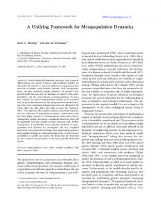
兵 a j 其 of all other pools j. Because all neurons participate in FIG. 2. A graded-response model including refractory effects, according to Ref. 关17兴. In this model, the neurons of a single pool can be grouped into three subpopulations: neurons that fired recently (a), neurons that are in a relative refractory state (r), and neurons that are quiescent (q). Neurons from a decay with a rate ␣ toward the state r, and neurons from r decay with a rate ␤ toward the state q. A synaptic field h induces field-dependent transitions from the refractory 共r兲 or the quiescent 共q兲 subpopulation toward the firing 共a兲 subpopulation with rates ␴ 1 (h) and ␴ 2 (h), respectively. With an appropriate a-dependent field h, a single recursively coupled pool can generate sustained oscillations.

graded-response models. We will also show how gradedresponse models can be incorporated into a broader framework of pool activity dynamics which allows for a comparison of the dynamics parameters with single-neuron parameters. B. Graded-response models with refractory effects

The necessity of having at least two variables for the generation of oscillatory pool behavior has been exploited in another graded-response-like model that relies upon a more realistic neuronal basis 关17兴. Instead of a second pool as in Eqs. 共5兲, a subpopulation of refractory neurons 共which are refractory because of recent spiking兲 takes care of the inhibitory effects. Consider a pool i with pool neurons that can be in either of three different states: active, refractory, and quiescent. They can be active, which means that they released a spike in a certain past time interval; they can be in a refractory state 共after firing兲; or they can be quiescent, that is, they do not fire and do not feel the refractory effects anymore. Between the three states, transitions are allowed with a certain probability. We define a i as the number of neurons of pool i that fired recently, r i as the number of pool neurons that are in the refractory state, and q i as the number of quiescent pool neurons. Neurons from the a i subpopulation decay toward the refractory state with a rate ␣ ; similarly, neurons from the r i subpopulation decay toward the quiescent state with a rate ␤ . On the other hand, neurons from the quiescent and refractory subpopulations can be activated by a synaptic input field h i with transition rates ␴ 1 (h i ) and ␴ 2 (h i ), respectively, with ␴ 1 (h i )⭐ ␴ 2 (h i ). The three states with their subpopulations and the allowed transitions are illustrated in Fig. 2. Assuming a first-order decay between the three subpopulations, we find d a 共 t 兲 ⫽⫺ ␣ a i 共 t 兲 ⫹q i 共 t 兲 ␴ 1 关 h i 共 t 兲兴 ⫹r i 共 t 兲 ␴ 2 关 h i 共 t 兲兴 , dt i

共6兲

the process, we have q i (t)⫹a i (t)⫹r i (t)⫽1, so that only two quantities are independent: d a 共 t 兲 ⫽⫺ ␣ a i 共 t 兲 ⫹ 兵 1⫺a i 共 t 兲 ⫺r i 共 t 兲其 ␴ 1 关 h i 共 t 兲兴 dt i ⫹r i 共 t 兲 ␴ 2 关 h i 共 t 兲兴 , d r 共 t 兲 ⫽ ␣ a i 共 t 兲 ⫺r i 共 t 兲兵 ␤ ⫹ ␴ 2 关 h i 共 t 兲兴其 . dt i

共9兲共10兲

Neurons that release a spike participate in the a i (t) subpopulation for a short time period. Afterwards, they enter the refractory phase, during which the probability of a new spike release ␴ 1 (h i ) due to the input field h i is low. After a longer time period without spiking, the refractory effects disappear, and the neuron can release a new spike with a greater probability ␴ 2 (h i )⭓ ␴ 1 (h i ). In this model, we have written a i (t) instead of A i (t), because we are dealing with the total number of spikes released during a certain period of time, instead of the spike density. This means that a i (t)⬇ ␶ A i (t), with some time constant ␶ . This creates a difficulty in the normalization condition q i (t)⫹a i (t)⫹r i (t)⫽1 and in the interpretation of the outcome of simulations within this model. Similarly, it is difficult to identify the parameters of the model with experimental data. Again, after the derivation of our pool dynamics, we will see that the pool model of this subsection can be understood as an approximation of a more general pool dynamics. III. MICROSCOPIC MODEL: SPIKING NEURONS

In this section we introduce the basic notions that define a pool dynamics. A. Single spiking neurons

Imagine a pool composed of extensively many NⰇ1 neurons with the same neuronal dynamics parameters. Inspired by the three-state system description of Ref. 关17兴 presented in Sec. II B, we now introduce a three-state neuron. A single neuron i, 1⭐i⭐N, can be in one of three different states: it can be inactivated (i), it can be activated (a), or it can be firing ( f ). A neuron can only fire, i.e., release an action potential 共or spike兲, if it is activated. If this is the case, the neuron fires with some probability ⌬t/ ␶ 关 h i (t) 兴 during the interval (t,t⫹⌬t 兴 , depending on its synaptic input field h i (t). After the release of a spike, the neuron is to remain inactivated for a certain time period of length ␥ abs. During this period it cannot spike, so that it is in an absolute refractory state. Following the absolute refractory period, the neuron enters a relative refractory period during which the neu-

1858


PRE 61

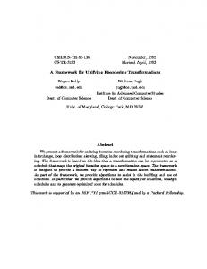
tion function.’’ It is divided into two parts. For a period of length ␥ abs, we have the absolute refractory period, with p A (s)⫽0 and s⫽t⫺t * i the elapsed time since the last spike. After that period, the neuron enters the relative refractory period, during which p A (s) rises from some value p A ( ␥ abs) toward 1 for s→⬁, according to a differentiable function P A (s). Between the two refractory periods, we allow a discontinuity of the function p A (s) at ␥ abs: p A共 s 兲 ⫽ FIG. 3. Definition of the microscopic model of a spiking neuron. In our description, a neuron can be in either of three states: inactivated (i), activated (a), or firing ( f ). Transitions between the three states are allowed between the i and the a levels 共fast, with transition rates that depend on the last spike time t * ), from the a level to the f level 关slow, with a transition rate that depends on the synaptic input field h(t)] and from the f level back to the i level 共fast兲. The mean occupation of the a level is given by the activation probability p A (t⫺t * ). Refractoriness means the neuron bounces back and forth between the i level and the a level, with 1⬎p A (t⫺t * )⭓0. A neuron can only release a spike if it is activated (a). The firing probability for activated neurons in a time interval of length ⌬t is field dependent and equal to ⌬t/ ␶ 关 h(t) 兴 . After firing, t * is reset and the neuron is inactivated.

ron has a certain probability p A ⬎0 of being activated, and thus a nonvanishing total probability for a spike release. We assume that only the time elapsed since the very last spike of a neuron at t i* determines its refractoriness, so that we end up with an activation probability 1⬎p A (t⫺t i* )⭓0 for t ⭓t * i . This is the ‘‘renewal hypothesis’’ for spiking neurons; see e.g., Ref. 关2兴. Figure 3 shows the three possible internal states of a single neuron and the allowed transitions. We assume the transitions of a neuron’s state between the inactivated state and the activated state to occur on a fast time scale as compared to the transition of a neuron from the activated state to the firing state and the modification of the activation probability with time. It is therefore sufficient to regard the mean occupation p A of the activated state of a neuron. From the activated state, and depending on the synaptic input field h i (t), a neuron can be pushed into the firing state with a rate 兵 ␶ 关 h i (t) 兴其 ⫺1 . A neuron in the firing state releases a single spike, and drops immediately back into the inactivated state. In summary, the total firing probability of a neuron i during an interval (t⫺⌬t,t 兴 is given by the joint probability that a neuron is in an activated state and that it is pushed into the firing state by the synaptic field h i (t) during that time interval:

⫽Prob 兵i fires in 共 t,t⫹⌬t 兴 due to field h i 兩 i苸a 其 ⌬t ⫻Prob 兵i苸a 其 ⫽ p 共 t⫺t * i 兲. ␶ 关 h i 共 t 兲兴 A

for 0⭐s⬍ ␥ abs

P A共 s 兲

共12兲

The synaptic field of a single neuron is calculated as follows. Each pool neuron releases a series of action potentials, each of which, after a fixed delay period, reaches a synapse of another neuron. This causes a temporal variation of the membrane potential at the postsynaptic neuron. The total variation of the postsynaptic membrane potential due to incoming action potentials is the synaptic field h i (t). Since we assume passive conducting characteristics of the dendritic tree, the synaptic field is calculated as a sum of the contributions of single action potentials. If we neglect the form of a spike we can characterize action potentials uniquely by their firing times t if , with f ⭓1. Here t 1i ⫽t * i is the most recent action potential of a neuron i in a spike train of ␦ functions, S i共 t 兲 ⫽

兺f ␦ 共 t⫺t if 兲 ,

共13兲

with t if ⭐t. The synaptic field is then calculated by inserting the coupling strength J i j for connections from neuron j to neuron i and fixing the temporal variation of the postsynaptic membrane potential ␣ (s):

兺 J i j 冕0 ds ␣ 共 s 兲 S j 共 t⫺s 兲 . j⫽1 N

h i共 t 兲 ⫽

⬁

共14兲

It may be well to realize that we have defined pool neurons to have the same input-output connectivity characteristics. This means that all neurons i of the same pool x feel the same synaptic field h(x,t). If the coupling strength from a connection conveying signals from a neuron j苸y of pool y to a neuron i苸x of pool x is designated with J(x,y), we get h 共 x,t 兲 ⫽

兺y j苸y 兺 J 共 x,y兲冕0 ds ␣ 共 s 兲 S j 共 t⫺s 兲 ⬁

兺y J 共 x,y兲冕0 ds ␣ 共 s 兲 A 共 y,t⫺s 兲 , ⬁

共15兲

with the pool activity

共11兲

The refractory properties are governed by the time course of the activation probability function 1⬎p A (t⫺t * i )⭓0, which in this paper will also be called in short the ‘‘activa-

for s⭓ ␥ abs.

B. Synaptic field

⫽

Prob 兵i苸a and i fires in 共 t,t⫹⌬t 兴 due to field h i 其

再

0

A 共 x,t 兲 ⫽

兺 S j共 t 兲.

j苸x

共16兲

The pool activity A(x,t) has the dimension spikes to time and is extensive; if desired, it can be normalized. The inte-

PRE 61


gration of A(x,t) over a small time interval of length ⌬t is then the total number of released spikes of all pool neurons during that interval. The time course of the membrane potential variation due to the input of a single spike follows qualitatively the form of an ␣ function: It rises to a maximum value and then decays back toward zero. In our case, the kernel ␣ (s) will be chosen to be a ␦ function, ␣ (s)⫽ ␦ (s⫺⌬ ax), so that h(x,t) ⫽ 兺 yJ(x,y)A(x,t⫺⌬ ax) or to have a Poisson-like time course ␣ (s)⫽ ␣ (k) (s) with 共 s⫺⌬ 兲 exp关 ⫺ 共 s⫺⌬ ax兲 / ␶ ␣ 兴 . ck ax k

␣ (k) 共 s 兲 ⫽⌰ 共 s⫺⌬ ax兲

共17兲

1859

d 1 D h 共 x,t,t * 兲 ⫽⫺ p 共 x,t⫺t * 兲 D h 共 x,t,t * 兲 . dt ␶ 关 h 共 x,t 兲兴 A

共19兲

Integration including the boundary condition D h (x,t * ,t * ) ⫽1 yields the ‘‘survival function’’ 关1兴

再

D h 共 x,t,t * 兲 ⫽ exp ⫺

冕

t

t*

dt ⬘

1

␶ 关 h 共 x,t ⬘ 兲兴

冎

p A 共 t ⬘ ⫺t * 兲 , 共20兲

that is a measure of the fraction of neurons that have spiked last at t * and did not spike again until t. B. Time evolution of the pool-averaged activity

Here ␶ ␣ is the rise time, s the time difference to the firing of the presynaptic neuron, c k the normalization factor, ⌬ ax the axonal delay time between two pools, and ⌰ the Heaviside step function 关 ⌰(x)⫽1 for x⭓0, and 0 otherwise兴. The constant c k can be used to normalize the alpha function by its maximum amplitude or its area. The maximum of the ␣ function is attained at s max⫽⌬ ax⫹k ␶ ␣ , and is equal to ␣ max⫽(k ␶ ␣ ) k e ⫺k . The area of the function gives F ␣ ⫽ ␶ ␣k⫹1 ⌫(k⫹1) with ⌫(k⫹1)⫽k! for k苸N. The pool form of the synaptic field, viz. the last of Eqs. 共15兲, will be used in the following sections for the formulation of our pool dynamics.

n 共 x,t,t * 兲 ⌬t * ⫽D h 共 x,t,t * 兲 A 共 x,t * 兲 ⌬t * .

The present section is devoted to a derivation of the time evolution of the key variable A(x,t), the activity. To this end, we start with the survival function that tells us how long a neuron survives without spiking. This will allow us to obtain an expression for calculating A(x,t), viz. Eq. 共26兲, which constitutes the key to the ensuing analysis. A. Survival function

In a pool of extensively many equivalent neurons, we take advantage of the property that all neurons of a pool x feel a common synaptic field. We now group the pool neurons into subgroups with the same last firing times t * ; for example, n(x,t,t * )⌬t * is the total number of pool neurons i苸x found at time t with t i* 苸(t * ⫺⌬t * ,t * 兴 . For times t⭓t * , we can then look at the time development of these subgroups. Let S h (x,t,t * ) be the fraction of a group of neurons that has spiked at least once during (t * ,t 兴 „the suffix h denotes a functional dependence of the function upon the field h(t ⬘ ) during the past time t ⬘ 苸(t * ,t 兴 …. Then this fraction changes in the interval (t⫺⌬t,t 兴 by

⫽

Taking the limit ⌬t→0, we obtain, for the time derivative of the fraction of neurons that did not spike again during (t * ,t 兴关i.e., of D h (x,t,t * )ª1⫺S h (x,t,t * )],

冕冕

t

⫺⬁ ⬁

0

dt * D h 共 x,t,t * 兲 A 共 x,t * 兲

dsD h 共 x,t,t⫺s 兲 A 共 x,t⫺s 兲 .

共22兲

By exploiting the same kind of argument, we can calculate another important macroscopic pool variable. The mean fraction of activated pool neurons that have spiked for the last time at t * is given by p A (t⫺t * ). Therefore, the mean number of inactivated neurons under the same conditions is 1⫺p A (t⫺t * ). The number of pool neurons that spiked last during (t * ⫺⌬t,t * 兴 and that are inactivated at time t is then n I共 x,t,t * 兲 ⌬t * ⫽ 关 1⫺ p A 共 t⫺t * 兲兴 D h 共 x,t,t * 兲 A 共 x,t * 兲 ⌬t * . 共23兲 From this we can calculate the total number of inactivated neurons of the pool: N I共 x,t 兲 ⫽ ⫽

共18兲

共21兲

Taking the limit ⌬t * →0 and adding over all possible last firing times t * 共that is, over all possible refractory states of the pool neurons兲, we obtain the total number of pool neurons: N 共 x兲 ⫽

IV. POOLS OF SPIKING NEURONS

⌬t p 共 t⫺t * 兲关 1⫺S h 共 x,t,t * 兲兴 . ⌬S h 共 t,t * 兲 ⫽ ␶ 关 h 共 x,t 兲兴 A

Using the survival function, we can now calculate n(x,t,t * )⌬t * . It is equal to the number of neurons A(x,t * )⌬t * that actually spiked during the interval (t * ⫺⌬t * ,t * 兴 , multiplied by the fraction of surviving neurons at time t:

冕冕

t

⫺⬁ ⬁

0

dt * 关 1⫺ p A 共 t⫺t * 兲兴 D h 共 x,t,t * 兲 A 共 x,t * 兲

ds 关 1⫺ p A 共 s 兲兴 D h 共 x,t,t⫺s 兲 A 共 x,t⫺s 兲 . 共24兲

The number of pool neurons that can contribute to the activity A(t⫹⌬t)⌬t during the next time step (t,t⫹⌬t 兴 is given by the total number of activated neurons, N(x)⫺N I(x,t). Because the activated neurons contribute to spiking with a probability 兵 ␶ 关 h(x,t) 兴其 ⫺1 ⌬t, for the activity we obtain

1860


A 共 x,t⫹⌬t 兲 ⌬t⫽

⌬t 关 N 共 x兲 ⫺N I共 x,t 兲兴 . ␶ 关 h 共 x,t 兲兴

共25兲

This equation is valid as long as A(x,t⫹⌬t)⌬tⰆN I(x,t). That is to say, as long as N I(x,t) can be considered as approximately constant during a time interval of length ⌬t. We note that in this case the activation A(x,t⫹⌬t) does not depend on the length of the time interval ⌬t. For any small enough ⌬t, the result will be the same. Hence we can take the limit ⌬t→0: A 共 x,t 兲 ⫽

1 关 N 共 x兲 ⫺N I共 x,t 兲兴 . ␶ 关 h 共 x,t 兲兴

共26兲

This is a nonlinear integral equation for the time evolution of the activity A(x,t); cf. Eq. 共25兲. It is the central equation from which we derive the pool dynamics. The nonlinearity of Eq. 共26兲 is hidden in the synaptic field h(x,t), which can depend on the activities of all other pools that provide synaptic input, including itself 关according to the second line of Eq. 共15兲 in Sec. III B兴. Starting from this equation, we will gain a differential equation system that describes the dynamics contained implicitly in Eq. 共26兲 and that is better suited to analytical treatment and numerical simulations. This will provide us with a straightforward and natural description of the activity dynamics of neuronal assemblies. In addition, the differential equation form will allow us to compare the system with the models discussed in Sec. II.

PRE 61

These equations have been calculated by differentiating repeatedly the field h (k) (x,t) and by extracting the terms of the additional fields h (l) (x,t). The coupling with other pools enters the differential equation system only in the second of Eqs. 共28兲. A similar procedure can be used if a sum of several ␣ functions of the type ␣ (k) (s), k苸N, is used as synaptic kernel. In this case, separate differential equation systems of the form of Eqs. 共28兲 have to be used to compute the different field contributions. The corresponding fields h (k) (x,t) have then to be added. This also opens the possibility to approximate ␣ functions with delay by weighted additions of ␣ functions without delay, thus resulting in a differential equation system without delay for the synaptic field. For k苸N, the integral equation 关the second line of Eq. 共15兲兴 instead of the differential equations 共28兲 has to be used. B. Activation probability functions

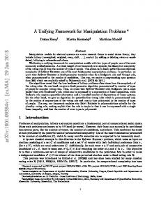
The behavior of a neuron i during its relative refractory period 共see Sec. III A兲 is characterized by the differentiable function P A (s), with s⫽(t⫺t * i ). From now on, we will restrict ourselves to the exponential case 共exp兲, the case of a sigmoidlike time evolution of the activation function after the absolute refractory period 共sigm兲, and the case of an inverse decay 共inv兲: P A共 s 兲 ⫽

再

1⫺ p 0 exp关 ⫺ 共 s⫺ ␥ abs兲 / ␶ ref兴 , 1⫺p 0 / 兵 1⫹ exp关共 s⫺s 0 兲 / ␶ ref兴其 , 1⫺ ␶ ref / 共 s⫺s 0 兲 ,

exp sigm

inv.

V. DIFFERENTIAL EQUATION POOL DYNAMICS

In this section, we are going to reduce the integral equations for the pool synaptic field h(x,t) and the pool activity A(x,t) to a system of coupled differential equations. We begin with the synaptic field because its derivation is straightforward. Then we derive the dynamics of the pool activity.

The constants p 0 , ␶ ref , and s 0 are free parameters of the activation function. It has to be verified that 0⭐ P A (s)⭐1 for ␥ abs⭐s⭐⬁; for example, for the inverse activation function in Eq. 共29兲, this means that we effectively set ␥ abs ⬎ ␶ ref⫹S 0 . The activation functions obey the differential equation

A. Synaptic field

The aim of this section is to express the synaptic field acting on the neurons of a specified pool through differential equations. For a synaptic field calculated according to the second line of Eqs. 共15兲, with an ␣ kernel of the type ␣ (s) ⫽ ␣ (k) (s), k苸N from Eq. 共17兲, we define additional fields h (l) 共 x,t 兲 ⫽

兺y

J 共 x,y兲

冕

⬁

0

ds ␣ (l) 共 s 兲 A 共 y,t⫺s 兲 ,

共27兲

with l苸N, 0⭐l⭐k. With this definition, the field we are looking for is h (k) (x,t), and it is straightforward to see that the field dynamics can be expressed by the differential equation system c l⫺1 (l⫺1) 1 d (l) h h 共 x,t 兲 ⫽l 共 x,t 兲 ⫺ h (l) 共 x,t 兲 , dt cl ␶␣ d (0) h 共 x,t 兲 ⫽ dt

兺y

1 J 共 x,y兲 A 共 y,t⫺⌬ ax兲 ⫺ h (0) 共 x,t 兲 . ␶␣

共28兲

共29兲

d P 共 s 兲⫽ ds A

冦

1 关 1⫺ P A 共 s 兲兴 , ␶ ref

exp

1 关 1⫺ P A 共 s 兲兴兵 1⫺ 关 1⫺ P A 共 s 兲兴 /p 0 其 , ␶ ref 1 关 1⫺ P A 共 s 兲兴 2 , ␶ ref

sigm

inv. 共30兲

These properties will be used in the subsequent sections for the derivation of the model. Figure 4 shows the different activation functions. C. Time evolution of the number of inactivated neurons

Here and in Sec. V D, we will reduce the integral equation for the pool activity 关Eq. 共26兲兴 to a differential equation system. To this end, we consider the time development of the total number of inactivated neurons N I(x,t). We use the t * form of Eq. 共24兲, the property d/dtD(x,t,t * ) ⫽⫺ 兵 ␶ 关 h(x,t) 兴其 ⫺1 p A (t⫺t * )D(x,t,t * ), and note that for a function of the type h(t,t * ) we have


PRE 61

d N 共 x,t 兲 ⫽A 共 x,t 兲 ⫺ dt I

冕冋 ⬁

ds

0

⫻A 共 x,t⫺s 兲 ⫺ FIG. 4. The different activation functions p A (t⫺t * ) used for the derivation of the pool dynamics. At s⫽ ␥ abs, the function may have, and here has, a discontinuity. For t&t * , the neuron is in an absolute refractory state because it has just spiked, and p A (t⫺t * )&0. For t→⬁, the refractory effects vanish, and p A (t⫺t * )→1. In case of activation functions with a discontinuity, ␥ abs is the length of the absolute refractory period.

d dt

冕

g(t)

f (t)

dt * h 共 t,t * 兲 ⫽F 关 t, f 共 t 兲兴 f ⬘ 共 t 兲 ⫺F 关 t,g 共 t 兲兴 g ⬘ 共 t 兲 ⫹

冕

g(t)

dt *

f (t)

⳵ h 共 t,t * 兲 , ⳵t

so, as

⫻

⫺

冦

1 ␶ ref 1 ␶ ref

冕冕冕

⬁

␥ abs ⬁

␥ abs ⬁

␥ abs

再

0

1 ␶ 关 h 共 x,t 兲兴

ds 关 1⫺ p A 共 s 兲兴 p A 共 s 兲 D h 共 x,t,t⫺s 兲共31兲

Thus the number of inactivated neurons grows with A(x,t). This makes sense, because neurons that spike are inactivated immediately afterwards. On the other hand, the number of inactivated neurons decreases with time as the refractory effect on neurons decreases. Moreover, the term p A (s) 关 1 ⫺p A (s) 兴 selects a time window of the activity that contributes to further changes of N I(x,t). Exploiting the properties 关Eq. 共30兲兴 of the chosen activation functions 共29兲 of Sec. V B, and taking into account the discontinuity of p A (s) at s⫽ ␥ abs, we obtain

冕

⬁

0

ds P A 共 s 兲关 1⫺ P A 共 s 兲兴 D h 共 x,t,t⫺s 兲 A 共 x,t⫺s 兲

ds 关 1⫺ P A 共 s 兲兴 D h 共 x,t,t⫺s 兲 A 共 x,t⫺s 兲 ds 关 1⫺ P A 共 s 兲兴 1⫺

⬁

册

d p 共 s 兲 D h 共 x,t,t⫺s 兲 ds A

⫻A 共 x,t⫺s 兲 .

1 d N I共 x,t 兲 ⫽A 共 x,t 兲 ⫺ P A 共 ␥ abs兲 A 共 x,t⫺ ␥ abs兲 ⫺ dt ␶ 关 h 共 x,t 兲兴 1 ␶ ref

冕

1861

exp p A 共 s 兲

冎

关 1⫺ P A 共 s 兲兴 D h 共 x,t,t⫺s 兲 A 共 x,t⫺s 兲 p0

ds 关 1⫺ P A 共 s 兲兴 2 D h 共 x,t,t⫺s 兲 A 共 x,t⫺s 兲

sigm p A 共 s 兲

共32兲

inv p A 共 s 兲 .

Instead of P A (s), we want to express our dynamics using the original activation function p A (s). For this purpose, we introduce a quantity M 共 x,t 兲 ⫽

冕

␥ abs

0

dsD h 共 x,t,t⫺s 兲 A 共 x,t⫺s 兲 ⫽

冕

␥ abs

0

共33兲

dsA 共 x,t⫺s 兲 ,

which is interpreted as the number of inactivated neurons for a pool with absolute refractory period only, and rewrite the previous equation 共32兲 in the form 1 d N I共 x,t 兲 ⫽A 共 x,t 兲 ⫺p A 共 ␥ abs兲 A 共 x,t⫺ ␥ abs兲 ⫺ dt ␶ 关 h 共 x,t 兲兴

⫺

⫹

冦

1 ␶ ref 1 ␶ ref 1 ␶ ref

冕冕冕

⬁

0 ⬁

0 ⬁

0

冕

⬁

0

ds p A 共 s 兲关 1⫺ p A 共 s 兲兴 D h 共 x,t,t⫺s 兲 A 共 x,t⫺s 兲

ds 关 1⫺ p A 共 s 兲兴 D h 共 x,t,t⫺s 兲 A 共 x,t⫺s 兲

再

ds 关 1⫺ p A 共 s 兲兴 1⫺

冎

关 1⫺ p A 共 s 兲兴 D h 共 x,t,t⫺s 兲 A 共 x,t⫺s 兲 p0

ds 关 1⫺ p A 共 s 兲兴 2 D h 共 x,t,t⫺s 兲 A 共 x,t⫺s 兲

1 M 共 x,t 兲 . ␶ ref

exp p A 共 s 兲 sigm p A 共 s 兲

inv p A 共 s 兲

共34兲


1862

PRE 61

What is the relevance of this equation? Since the dynamics of A(x,t) is determined by the dynamics of h(x,t) and of N I(x,t), it is of primary importance to understand the time development of the number of inactivated neurons. In the next section 共V D兲, we will see how this allows us to derive systematically a system of differential equations for the dynamics of A(x,t). D. Pool dynamics

The number N I(x,t) of inactivated neurons of a pool is the assembly-averaged mean inactivation probability. For the calculation of the mean, we need the momentary density ␳ (x,t,t * )⫽D h (x,t,t * )A(x,t * ) of neurons with a refractory state defined by their last spike at t * . With this density and the definition

具 ••• 典 ª

冕

t

⫺⬁

FIG. 5. The activation function p A (s) is shown with its recovery kernels 关 1⫺p A (s) 兴 m . With growing m, the kernels include less and less of the past time s. The pool dynamics is expressed with the help of a series of recovery variables N m (x,t)ª 具关 1⫺p A (t⫺t * ) 兴 m 典 calculated by computing the pool average of the recovery kernel function.

N (m) 共 x,t 兲 ª 具关 1⫺ p A 共 t⫺t * 兲兴 m 典 , so that, for m苸N,

dt * ␳ 共 x,t,t * 兲 •••,

共35兲 N (m) 共 x,t 兲 ⫽

we can write N I共 x,t 兲 ⫽ 具 1⫺ p A 共 t⫺t * 兲典 .

N

共 x兲 ⫽ 具关 1⫺ p A 共 t⫺t * 兲兴典 , 0

N (1) 共 x,t 兲 ⫽ 具关 1⫺ p A 共 t⫺t * 兲兴 1 典 ,

⫽

共36兲

The kernel 1⫺p A (t⫺t * ) determines the influence of the past activity on the quantity N I(x,t). Instead of using integral equations which incorporate the past activity by means of equidistant time slices 共imagine a Riemann sum approximation of the integral equations兲, we could try to incorporate the past using a set of kernels similar to 1⫺p A (t⫺t * ). The underlying problem is that of the reducibility of an integrodifferential equation to a system of differential equations. It has been treated by a number of authors, e.g., see, Refs. 关18,19兴. In principle, a reduction of Eqs. 共31兲 or 共34兲 into a chain of differential equations is possible for a suitable choice of intermediary variables. The problem is that there is no systematic derivation of these additional variables, so that we have to guess. As indicated above we will use the function 1⫺p A (t⫺t * ) for this purpose. To accomplish the reduction of Eq. 共34兲, the number of inactivated neurons N I(x,t) will be treated in a way equivalent to N (1) (x,t), the total number of pool neurons N(x) will be handled as N (0) (x), and the number M (x,t) of inactivated neurons for a pool with absolute refractory period only, as N (⬁) (x,t). Furthermore, we remark that definition 共22兲 of N(x)⫽N (0) (x), definition 共24兲 of N I(x,t)⫽N (1) (x,t), and definition 共33兲 of M (x,t)⫽N (⬁) (x,t) are equivalent to (0)

共38兲

共37兲

N (⬁) 共 x,t 兲 ⫽ 具关 1⫺ p A 共 t⫺t * 兲兴 ⬁ 典 . Extending these definitions, we introduce additional timedependent inactivation quantities, or ‘‘recovery variables’’

冕冕

t

⫺⬁ ⬁

0

dt * 兵 1⫺ p A 共 t⫺t * 兲其 m D h 共 x,t,t * 兲 A 共 x,t * 兲

ds 兵 1⫺ p A 共 s 兲其 m D h 共 x,t,t⫺s 兲 A 共 x,t⫺s 兲 . 共39兲

N (m) (x,t) obeys the relationship N (0) 共 x兲 ⭓N (1) 共 x,t 兲 ⭓N (2) 共 x,t 兲 ⭓•••⭓N (⬁) 共 x,t 兲 ᭙t,

共40兲

and has the property

冕

⬁

0

ds 兵 1⫺ p A 共 s 兲其 m p A 共 s 兲 D h 共 x,t,t⫺s 兲 A 共 x,t⫺s 兲 ⫽N (m) 共 x,t 兲 ⫺N (m⫹1) 共 x,t 兲 .

共41兲

Figure 5 shows an example of a sigmoidal activation function p A (s) with an absolute refractory period of length ␥ abs and the recovery kernels 关 1⫺ p A (s) 兴 m . For these recovery variables, we can calculate the time derivative in the same way as for N I(x,t) in Eq. 共31兲: d (m) N 共 x,t 兲 ⫽A 共 x,t 兲 ⫺m dt

冕

⫻

冋

⫺

1 ␶ 关 h 共 x,t 兲兴

⬁

0

ds 关 1⫺ p A 共 s 兲兴 m⫺1

册

d p 共 s 兲 D h 共 x,t,t⫺s 兲 A 共 x,t⫺s 兲 ds A

冕

⬁

0

ds 关 1⫺ p A 共 s 兲兴 m p A 共 s 兲

⫻D h 共 x,t,t⫺s 兲 A 共 x,t⫺s 兲 .

共42兲

Finally, with property 共41兲, we obtain a recursive set of differential equations:

PRE 61


1863

d (m) 1 N 共 x,t 兲 ⫽A 共 x,t 兲 ⫺ 兵 1⫺ 关 1⫺ p A 共 ␥ abs兲兴 m 其 A 共 x,t⫺ ␥ abs兲 ⫺ 关 N (m) 共 x,t 兲 ⫺N (m⫹1) 共 x,t 兲兴 dt ␶ 关 h 共 x,t 兲兴

⫺

冦

m 关 N (m) 共 x,t 兲 ⫺M 共 x,t 兲兴 ␶ ref

exp p A 共 s 兲

m 兵 N (m) 共 x,t 兲 ⫺M 共 x,t 兲 ⫺ 关 N (m⫹1) 共 x,t 兲 ⫺M 共 x,t 兲兴 /p 0 其 ␶ ref m 关 N (m⫹1) 共 x,t 兲 ⫺M 共 x,t 兲兴 ␶ ref

sigm p A 共 s 兲

共43兲

inv p A 共 s 兲 .

The last recovery variable N (⬁) (x,t)⫽M (x,t) increases with the number of spiking neurons, and decreases with the number of neurons that are released from their absolute refractory phase:

The remaining axonal delay in Eqs. 共28兲 can be avoided using the procedure for synaptic fields with ␣ functions with delay as explained in Sec. V A.

d M 共 x,t 兲 ⫽A 共 x,t 兲 ⫺A 共 x,t⫺ ␥ abs兲 . dt

VI. CONSEQUENCES

共44兲

This completes our derivation of the pool dynamics. System 共43兲 looks linear but it is not since the field h(x,t) 关Eqs. 共28兲兴 contains the recovery variable N (1) (x,t) through the activity A(x,t). The complete dynamics is defined by the field dynamics given by Eqs. 共28兲 of Sec. V A together with the dynamics of the recovery variables given by Eqs. 共43兲 and 共44兲. The spike density acts only as an auxiliary variable that is calculated from the first recovery variable using the main equation 共26兲 of Sec. IV B A 共 x,t 兲 ⫽

1 关 N 共 x兲 ⫺N (1) 共 x,t 兲兴 . ␶ 关 h 共 x,t 兲兴

共45兲

Other pools y influence the dynamics of pool x through A(y,t) in the last equation of the field h(x,t) in Eqs. 共28兲. Axonal delays appear in the second of Eqs. 共28兲, in the dynamics of the recovery variables 共43兲 due to the discontinuity of p A (s) at ␥ abs, and in Eq. 共44兲 also because of the absolute refractory period. To model pool dynamics using differential equations without delays, a differentiable activation function p A (s) without absolute refractory period has to be chosen. In this case, system 共43兲 reduces to d (m) N 共 x,t 兲 dt ⫽A 共 x,t 兲 ⫺

⫺

冦

1 关 N (m) 共 x,t 兲 ⫺N (m⫹1) 共 x,t 兲兴 ␶ 关 h i 共 x,t 兲兴

m (m) N 共 x,t 兲 ␶ ref

exp p A 共 s 兲

m 关 N (m) 共 x,t 兲 ⫺N (m⫹1) 共 x,t 兲 /p 0 兴 sigm p A 共 s 兲 ␶ ref m (m⫹1) N 共 x,t 兲 ␶ ref

inv p A 共 s 兲 . 共46兲

In this section, we are going to analyze in detail the consequences that follow from using the system 共43兲 for the calculation of assembly dynamics. System 共43兲 is exact for assemblies composed of extensively many spiking neurons. Nevertheless, for a numerical implementation of the dynamics, the infinite chain of differential equations has to be approximated by a finite differential equation system. Breaking the chain earlier or later leads to a dynamics that follows the exact result in a smooth fashion or in every detail. One can therefore approximate the pool dynamics with the desired accuracy. Here we discuss systematic approximations to the differential equation system and show simulation results for the different approximation schemes.

A. Systematic approximations

Contrary to previous work on pool dynamics, the present procedure is exact for pools of extensively many neurons since it does not rely upon time averaging for its derivation. This allows us to quantitatively model pool activities well beyond the quasistationary regime. But for numerical simulations, the infinite chain of differential equations has to be approximated by a finite system. Because of property 共40兲 of the recovery variables, we can approximate the infinite chain of differential equations 关system 共43兲兴 by breaking it at a desired recovery variable N (n⫹1) (x,t) and by introducing an appropriate dynamics for this quantity. In this section, we will proceed to analyze different approximations of the differential equation system for our pool model. There are two sensible ways of approximating N (n⫹1) (x,t), which differ according to the desired dynamical simulation range. Assuming that n is large enough, the influence of the relative refractory field on the (n⫹1)th recovery variable can be neglected, and we can approximate N (n⫹1) (x,t)⬇M (x,t); or N (n⫹1) (x,t)⬇0 if we are dealing with neurons without absolute refractory period. 共i兲 For fast, transient dynamics with sharp activity steps, N (n⫹1) (x,t) is then calculated according to the dynamics of M (x,t):


1864

d (n⫹1) d N 共 x,t 兲 ⬇ M 共 x,t 兲 ⫽A 共 x,t 兲 ⫺A 共 x,t⫺ ␥ abs兲 , dt dt

PRE 61

共47兲

or, for neurons without absolute refractory period, we use Eq. 共46兲 for d/dtN (n) (x,t) and N (n⫹1) (x,t)⬇0. In the case of exponential or sigmoidal p A (s), this gives for the nth recovery variable

冋

册

n 1 d (n) ⫹ N (n) 共 x,t 兲 . N 共 x,t 兲 ⬇A 共 x,t 兲 ⫺ dt ␶ 关 h 共 x,t 兲兴 ␶ ref

共48兲

共ii兲 For slow dynamics, we can approximate N (n⫹1) (x,t) by its stationary value. For slow dynamics, the activity A(x,t) and the field h(x,t) are approximately constant during the time period of the kernel 关 1⫺ p A (s) 兴 n⫹1 of N (n⫹1) (x,t). This means that N (n⫹1) 共 x,t 兲 ⬇ 关 ␥ abs⫹ ␬ (n⫹1) 共 x兲兴 A 共 x,t 兲 , h

共49兲

(x) being the time constant of the (n⫹1)th kerwith ␬ (n⫹1) h nel due to relative refractory effects:

␬ (n⫹1) 共 x兲 ⫽ h

冕

⬁

␥ abs

ds 关 1⫺ p A 共 s 兲兴 n⫹1 D h 共 x,t,t⫺s 兲 . 共50兲

(x) has been evaluated for a quasistationary field Here ␬ (n⫹1) h h(x,t) 共i.e., the field is assumed to be constant for a period during which the expression in the integral is large兲, and, thus, it is written without an explicit dependency on t. It depends, however, on the field h. For neurons with absolute refractory period only, ␬ (n⫹1) (x)⫽0, and we can use h N (n⫹1) (x,t)⬇ ␥ absA(x,t) as the stationary approximation. Similarly, in the case of pools with a relative refractory pe(x)A(x,t). The slow riod only, we use N (n⫹1) (x,t)⬇ ␬ (n⫹1) h approximation is exact when the activity approaches a stationary value. B. Zeroth-order approximation: stationary solution and gain function

For constant input field h(x,t)⬅h(x) and stationary activity A(x,t)⬅A(x), it is d/dtN (m) (x,t)⫽0 ᭙m, so that from the assembly dynamics 共43兲 and 共45兲 only remains A 共 x兲 ⫽

1 关 N 共 x兲 ⫺N (1) 共 x兲兴 . ␶ 关 h 共 x兲兴

共51兲

Using this equation, and expression 共49兲 for N (1) (x) in the stationary case, N (1) 共 x兲 ⫽ 关 ␥ abs⫹ ␬ (1) h 共 x 兲兴 A 共 x 兲 ,

共52兲

FIG. 6. The stationary spike density for a pool of spiking neurons which receives a constant synaptic input field h can be expressed by a gain function that is similar to the logistic gain function. Here we show the gain function for a pool of neurons with absolute refractory period only 共thin solid line兲, and for a pool with absolute and relative refractory period 共thick solid line兲. The relative refractory period reduces the activity for fields h close to the threshold 共dashed line: difference between the gain function without and the gain function including relative refractory effects兲.

With the often used ansatz ␶ 关 h 兴 ⫽ ␶ 0 exp关⫺2␤(h⫺␪)兴 with spike rate at threshold ␶ ⫺1 0 , noise parameter ␤ , and threshold ␪ 共see, e.g., Ref. 关1兴兲, we obtain G 关 x,h 共 x兲兴 ⫽

1

1

␥

abs

abs 1⫹ exp 兵 ⫺2 ␤ 关 h 共 x兲 ⫺ ␪ ⬘ 兴其 ⫹ ␬ (1) h 共 x兲 / ␥

,

共54兲 with the modified threshold

␪ ⬘ ⫽ ␪ ⫹1/共 2 ␤ 兲 ln共 ␶ 0 / ␥ abs兲

共55兲

and the relative refractory period time constant ␬ (1) h (x) as defined in Eq. 共50兲. Figure 6 shows the stationary spike density A(x) as a function of the synaptic field h(x). The pool spike rate A(x) saturates at N(x)/ ␥ abs as it is bounded by the inverse length of the absolute refractory period. The time constant ␬ (1) h (x) quantifies the influence of the relative refractory period on the stationary pool spike rate. It reduces the activity for intermediate fields h(x)⬇ ␪ . The noise factor ␤ and the effective threshold ␪ ⬘ determine the slope and the inflection point of the gain function. Increasing the length of the absolute refractory period ␥ abs or decreasing the firing rate at threshshifts the effective threshold toward higher values. old ␶ ⫺1 0 We see that the present model lets us understand the gain function quantitatively in terms of the microscopic neuronal parameters ␥ abs, ␬ (1) h , ␶ 0 , ␤ , and ␪ . This marks a difference to standard gain functions as those used with other gradedresponse pool models.

we can calculate the normalized stationary spike density to A 共 x兲 1 ⫽ . G 关 x,h 共 x兲兴 ª N 共 x兲 ␥ abs⫹ ␶ 关 h 共 x兲兴 ⫹ ␬ (1) h 共 x兲

共53兲

If ␶ 关 h 兴 is a monotonously decreasing function of h, we get a gain function G 关 h 兴 that saturates at large h and has a sigmoidal-like appearance.

C. First-order approximation: quasistationary dynamics and graded response

The graded-response models presented in Secs. II A and II B have a serious disadvantage: they have free dynamical parameters which can be chosen at will. Of course we could fit the model parameters with experimental data, but still it would be difficult to interpret the data, because the free pa-

PRE 61


rameters stem from the dynamics derivation procedure 共more precisely, from temporal averaging兲, and not from the microscopic properties of the neurons. Here we move in the opposite way. We start from our main equations 共43兲 and derive a closed expression for the simplest possible assembly dynamics. This results in a graded-response-like relaxation dynamics that follows smoothly and coarsely the real dynamics of the assembly. Additionally, all its parameters can be interpreted in terms of the microscopic neuronal parameters. Since we want to gain a relaxation dynamics without delays, we assume that there is no discontinuity in the activation function p A (s), i.e., the neurons have a relative refractory behavior but no absolute refractory period. We start with a first-order approximation of our main equations 共46兲. We use the slow-dynamics approximation 共49兲, and chop the differential equation system at n⫽1, so that N (2) 共 x,t 兲 ⬇ ␬ (2) h 共 x 兲 A 共 x,t 兲

共56兲

with ␬ (2) h (x) calculated as specified in Eq. 共50兲关depending on h(x,t)]. 共The slow dynamics approximation now involves temporal averaging. The difference to standard gradedresponse models is that the averaging occurs over intrinsic neuronal time intervals, and not a priori over some arbitrary interval of length T. Therefore, it does not introduce additional dynamical parameters. Moreover, since we look at slow, or even quasistationary, dynamics in this case, the temporal averaging is justified. We also remind that we can avoid temporal averaging if we use the fast dynamics approximation, resulting in a first-order approximation that has the form of a differential equation with delay.兲 This means that we only have two state variables, namely, the activity A(x,t) and the first recovery variable N (1) (x,t)⫽N I(x,t), which is the number of neurons in the inactivated state. The number of inactivated neurons is obtained from A(x,t) ⫽ ␶ 关 h(x,t) 兴 ⫺1 关 N(x)⫺N I(x,t) 兴 , so as to give N I共 x,t 兲 ⫽N⫺ ␶ 关 h 共 x,t 兲兴 A 共 x,t 兲 .

共57兲

We now turn to the activity A(x,t). We assume that, for quasistationary activity, the fields evolve more slowly than the activity, and neglect the changes of h(x,t). 关Without loss of generality, we can include a term that considers the variation of A(x,t) due to changes of h(x,t), so that this assumption is not really necessary for the calculation of first-order dynamics. It is omitted only to gain an equation that can be compared to other graded-response models.兴 This leaves us with d/dtA(x,t)⬇⫺ ␶ 关 h(x,t) 兴 ⫺1 d/dtN I(x,t), and inserting Eqs. 共56兲 and 共57兲 into the dynamics equation 共46兲 for N I(t) with exponential p A (s) 关the same steps can be applied to the other functions p A (s)], we arrive at

␶ g 关 h 共 x,t 兲兴

d A 共 x,t 兲 dt

⫽⫺A 共 x,t 兲 ⫹

冋

再

册冎

with 1 1 1 ⫽ ⫹ . ␶ g 关 h 共 x,t 兲兴 ␶ 关 h 共 x,t 兲兴 ␶ ref

共59兲

Not only has this graded-response-type equation the microscopically correct stationary solutions but it also provides us with the relaxation time constant ␶ g 关 h(x,t) 兴 . This means that if we are interested in a realistic quasistationary pool behavior, graded-response equations with fixed relaxation time constants as those of Secs. II A and II B are not sufficient. Equation 共58兲 is the correct way to introduce a systematically derived graded-response-type dynamics for pools of spiking neurons using the chain of differential equations. The effect of Eq. 共58兲 is a dynamics that follows the real activity dynamics by smoothing out sharp activity peaks. Nevertheless, it will do so following the envelope curve of the activity, and it will still approach the correct stationary solutions for a constant field h(x). D. Higher-order approximations: Realistic assembly dynamics

Higher-order approximations serve to model in a quantitatively accurate way the dynamics of assemblies of spiking neurons. Using the fast dynamics approximation 共47兲, the model is capable of reproducing the time-course of the activity of a pool composed of extensively many neurons, including fast transients and sharp activity peaks like those occurring when the activity approaches oscillatory solutions. The different recovery variables serve as memory buffers for the past activity. Higher 共with larger n) recovery variables are responsible for the more recent past, and influence the response of the pool to fast transients. Taking only one or two recovery variables results in activities that follow the real activity in a smooth, approximated way. If we include more recovery variables, the assembly dynamics also follows the smaller details of the real activity. Figures 7 and 8 show simulations of transient and oscillatory pool dynamics calculated using Eqs. 共43兲. The activity is compared with results gained from simulations using assemblies of explicitly modeled spiking neurons. VII. CONNECTION WITH OTHER MODELS

In this section, we compare the model with other neuronal models. Specifically, we show that standard gain functions and graded-response models can be understood in terms of our pool dynamics, and that this allows us to interpret the parameters of those functions in terms of the microscopic parameters of our underlying neuronal model. Furthermore, we show that our model is equivalent to a pool of spikeresponse or integrate-and-fire neurons. A. Gain function

1 N 共 x兲 ⫺ ␶ g 关 h 共 x,t 兲兴 ␶ 关 h 共 x,t 兲兴

␬ (2) h 共 x兲 ⫻ 1⫺ A 共 x,t 兲 , ␶ 关 h 共 x,t 兲兴

1865

共58兲

In Sec. VI B, we have shown that the stationary solution of the pool dynamics is the sigmoidal gain function 共54兲. In case we have an absolute refractory period only, ␬ (1) h (x) vanishes, and we obtain an equation of the same form as the standard logistic gain function:

1866


PRE 61

G 关 h 共 x兲兴 ⫽ ⫽

1

␥

abs

1 1⫹ exp 兵 ⫺2 ␤ 关 h 共 x兲 ⫺ ␪ ⬘ 兴其

1 1 共 1⫹tanh 兵 ␤ 关 h 共 x兲 ⫺ ␪ ⬘ 兴其兲 . ␥ abs 2

共60兲

Since A maxª1/␥ abs is the maximal spiking activity of the neurons, and normalizing the activity A→A/N, we obtain A 共 x兲 ⫽A max 21 „1⫹tanh 兵 ␤ 关 h 共 x兲 ⫺ ␪ ⬘ 兴其 ….

共61兲

This means that for pools of spiking neurons we can use the standard logistic gain function to obtain realistic stationary results, and we know how each parameter of the gain function can be interpreted in terms of the microscopic parameters of the underlying neuronal model. FIG. 7. Simulation of the activity A(t) of a single pool of neurons without couplings, using spike-response neurons 共solid line兲 or Eqs. 共43兲共dashed line兲. From 50 to 150 ms, a constant external field is applied 共black bar兲. The sudden onset of the external field evokes a sharp activity peak which decays in a damped oscillation towards the new stationary state. We have used the fast dynamics approximation with n⫽4 recovery variables and fast approximation N (4) (t)⬇N (⬁) (t), meaning d/dtN (4) (t)⫽A(t)⫺A(t⫺ ␥ abs), and fifth-order Runge-Kutta integration with adaptive stepsize. The simulations show a good quantitative agreement.

B. Standard graded-response models

The standard graded-response models of Sec. II A can be motivated as follows from our pool dynamics. We look at the normalized form (A→A/N) of Eq. 共45兲. In a quasistationary regime we define a dynamics by an exponential relaxation towards the stationary solution of Eqs. 共43兲 and 共45兲, given by A(x)⫽ ␶ 关 h(x) 兴 ⫺1 兵 1⫺ 关 ␥ abs⫹ ␬ (1) h (x) 兴 A(x) 其 :

␶

d 1 A 共 x,t 兲 ⫽⫺A 共 x,t 兲 ⫹ dt ␶ 关 h 共 x,t 兲兴 ⫻ 兵 1⫺ 关 ␥ abs⫹ ␬ (1) h 共 x 兲兴 A 共 x,t 兲其 .

共62兲

This equation, and its simpler variant 共for small 关 ␥ abs ⫹ ␬ (1) h (x) 兴 A(x,t)Ⰶ1)

␶

FIG. 8. Simulation of the activity A(t) of a single pool of reciprocally coupled neurons, using spike-response neurons 共solid line兲 or Eqs. 共43兲共dashed line兲. From 50 to 250 ms, a constant external field is applied 共black bar兲. The parameters of the pool neurons fulfill the locking theorem. The onset of the external field evokes a small activity peak, which grows and generates a selfsustained oscillation. As in the previous simulation, we have used the fast dynamics approximation with n⫽4. The simulations show a good quantitative agreement, except in the tips of the activity peaks 共finite-size effects兲.

d 1 A 共 x,t 兲 ⫽⫺A 共 x,t 兲 ⫹ , dt ␶ 关 h 共 x,t 兲兴

共63兲

are of the same form as the assembly-averaged gradedresponse models presented in Sec. II A. Equation 共62兲 will relax toward the correct microscopic solutions 共i.e., solutions that are in accordance with those obtained from simulations with single spiking neurons兲, incorporating absolute and relative refractory effects. There is no necessity of ‘‘timecoarse graining’’ or other temporal averaging procedures to arrive at Eq. 共62兲 for quasistationary activity. Gradedresponse models as in Eqs. 共62兲 and 共63兲 may thus present a valid approach, if the assembly dynamics are always close to the stationary state calculated from the microscopic parameters. For fast, transient, dynamics, the full differential equation system 共43兲 is to be used instead. Again, as in Sec. VI, it is now possible to understand how each parameter of the graded-response model can be interpreted in terms of the microscopic parameters of the underlying neuronal model. The only exception is the arbitrary relaxation time constant ␶ . For a calculation of the relaxation time constant using intrinsic neuronal parameters refer back to Sec. VI C. C. Graded-response models with refractory effects

We can enhance the standard graded response model 共62兲 by incorporating an additional term for the dynamics of the first recovery variable. Together with an exponential relax-

PRE 61


ation dynamics of A(x,t), using approximation 共48兲 for the number of inactivated neurons, and assuming neurons with relative refractory period only, we find

h i共 t 兲 ⫽

冋

册

1 1 d N 共 x,t 兲 ⫽A 共 x,t 兲 ⫺ ⫹ N 共 x,t 兲 . dt I ␶ 关 h 共 x,t 兲兴 ␶ ref I

共64兲

This system is similar to that of Sec. II B, Eqs. 共9兲 and 共10兲. Neurons can be firing, inactivated 共quiescent兲, and activated 共refractory兲. Between the three states transitions are allowed, some with a field-dependent rate and others with a fixed rate. Integrating the spike density over a small fixed interval T during which A(x,t) can be regarded as constant, we obtain the absolute number of neurons that released a spike recently, a(x,t)⬇TA(x,t). We further define r(x)ªN I(x,t), ␤ ª1/␶ ref , ␴ 1 关 h(x,t) 兴 ª„1/␶ 关 h(x,t) 兴 …(T/ ␶ ), ␴ 2 关 h(x,t) 兴 ª1/␶ 关 h(x,t) 兴 , ␣ a ⫽1/␶ , and ␣ r ⫽1/T, and rewrite Eqs. 共64兲 as d a 共 x,t 兲 ⫽⫺ ␣ a a 共 x,t 兲 ⫹ 兵 1⫺r 共 x,t 兲其 ␴ 1 关 h 共 x,t 兲兴 , dt d r 共 x,t 兲 ⫽ ␣ r a 共 x,t 兲 ⫺r 共 t 兲兵 ␤ ⫹ ␴ 2 关 h 共 x,t 兲兴其 . dt

⬁

兺f

␩ i 共 t⫺t if 兲 ⫽

冕

⬁

0

共67兲 ds ␩ i 共 s 兲 S i 共 t⫺s 兲 .

In this paper, we consider neurons with renewal. This means that only the last spike at t i* accounts for refractory effects, and thus contributes to h ref i (t): h ref i 共 t 兲 ⫽ ␩ i 共 t⫺t * i 兲.

共68兲

The ␣ (s) and ␩ (s) functions of the spike-response model can be used to model a broad range of types of neuronal models 共for the sake of simplicity, we will drop the neuron indices i and j of the ␣ and ␩ functions from here on兲. For example, it is possible to express the so-called ‘‘integrateand-fire’’ 共I&F兲 type models in terms of special functions ␣ (s) and ␩ (s). Using the total field of the SRM, we introduce an exponential total spike probability density 1/␶ SRM for neurons with renewal 关1兴, ref ␶ SRM关 h i 共 t 兲 ,h ref i 共 t 兲兴 ⫽ ␶ 0 exp 兵 ⫺2 ␤ 关 h i 共 t 兲 ⫹h i 共 t 兲 ⫺ ␪ 兴其

共65兲

⫽ ␶ 0 exp 兵 ⫺2 ␤ 关 h i 共 t 兲 ⫹ ␩ 共 t⫺t * i 兲 ⫺ ␪ 兲兴其 . 共69兲

The result is a system that is very similar to the model of Sec. II B. Again, we can interpret the parameters of the model in terms of their microscopic parameters. The system now depends, as in Sec. II B, on an arbitrary integration time constant T and a relaxation time constant ␶ . For quantitative modeling it is therefore better to use the assembly model presented in this paper, which is based exclusively on microscopic parameters. D. Connection with models of spiking neurons

In this subsection we compare one of the most general types of model of single-neuron threshold dynamics, the ‘‘spike-response model’’ 共SRM兲, with the presented pool model. We show how the parameters of our pool models can be mapped to parameters of the SRM. It turns out that our pool model is exact for pools of spike-response neurons with special refractory functions. In other cases, our model can be used as an approximation. In the SRM, the response of a neuron, say i, is determined by a total field that has two contributions: one from the synaptic inputs from other neurons and another that accounts for the neuron’s refractory behavior due to the release of action potentials, ref h total i 共 t 兲 ⫽h i 共 t 兲 ⫹h i 共 t 兲 .

兺j J i j 兺f ␣ i j 共 t⫺t fj 兲 ⫽ 兺j J i j 冕0 ds ␣ i j 共 s 兲 S j 共 t⫺s 兲 ,

h ref i 共 t 兲⫽

1 d ␶ A 共 x,t 兲 ⫽⫺A 共 x,t 兲 ⫹ 关 1⫺N I共 x,t 兲兴 , dt ␶ 关 h 共 x,t 兲兴

1867

共66兲

The neuron fires deterministically or with a certain probability, if the total field reaches a fixed threshold from below. The synaptic input field h i (t) is usually defined using an ␣ function as in Eq. 共14兲 of Sec. III B. The refractory field h ref i (t) is defined by a refractory function ␩ i (s). For spike trains of a neuron i, S i (t)⫽ 兺 f ␦ (t⫺t if ), we have

Then we can identify the spike probability density for activated neurons and the activation probability for refractory neurons from Sec. III A with

兵 ␶ 关 h i 共 t 兲兴其 ⫺1 ª ␶ ⫺1 0 exp 兵 2 ␤ 关 h i 共 t 兲 ⫺ ␪ 兴其

共70兲

p A 共 t⫺t * i 兲 ª exp 兵 2 ␤ ␩ 共 t⫺t * i 兲其.

共71兲

and

This means that the differential equation system for the pool dynamics 共43兲 is exact in the limit of pools composed of extensively many spike-response neurons with renewal and refractory functions ␩ (s) of the form

␩共 s 兲⫽

1 ln关 p A 共 s 兲兴 , 2␤

共72兲

with p A (s) being one of the activation functions presented in Sec. V B. Figure 9 shows an example of the exponential p A (s) and the corresponding refractory function calculated through Eq. 共72兲. Alternatively, we can start from frequently used refractory functions ␩ (s) and search for systematic approximations of these function through the corresponding p A (s). This is for example the case for I&F neurons, which use an exponential ␩ (s). Two of the most frequently used refractory functions are

␩ exp共 s 兲 ⫽

再

0 ⫺⬁

for s⬍0 for 0⭐s⬍ ␥ abs

冋

s⫺ ␥ abs ⫺ ␩ 0 exp ⫺ ␶␩

册

共73兲 for s⭓ ␥

abs


1868

FIG. 9. Correspondence between the activation function p A (s) 共solid line兲 and the negative refractory function ⫺ ␩ (s) of the SRM 共dotted line兲. In this case, we used an exponential p A (s) with an absolute refractory period of ␥ abs⫽1. At s⫽ ␥ abs, the refractory function ␩ (s) diverges to ⫺⬁.

and

␩ inv共 s 兲 ⫽

冦

0

for s⬍0 for 0⭐s⬍ ␥ abs

⫺⬁ ⫺

␶␩ s⫺ ␥ abs

for s⭓ ␥

共74兲

abs

.

For small ␩ (s), i.e., in the case that the synaptic field is small enough so that neurons do not spike again until their refractory field has already decreased considerably, we can approximate the activation function p A (s) in Eq. 共72兲 corresponding to the refractory function 共73兲 by p A 共 t⫺t * 兲 ⫽ exp关 2 ␤ ␩ 共 t⫺t * 兲兴 ⬇1⫹2 ␤ ␩ 共 t⫺t * 兲

冋

⫽1⫺2 ␤ ␩ 0 exp ⫺

册

s⫺ ␥ abs . ␶␩

共75兲

Comparing this with the exponential activation function or the sigmoidal activation function in Eq. 共29兲, we obtain p 0 ⫽2 ␤ ␩ 0 ,

␶ ref⫽ ␶ ␩

and

s 0 ⫽ ␥ abs.

共76兲

Similarly, in the case of the inverse refractory function 共74兲, we can approximate p A 共 t⫺t * 兲 ⫽ exp 兵 2 ␤ ␩ 共 t⫺t * 兲其 ⬇1⫹2 ␤ ␩ 共 t⫺t * 兲 ⫽1⫺2 ␤

␶␩ s⫺ ␥ abs

共77兲

,

and compare this with the inverse activation function 关the last of Eqs. 共29兲兴 so as to obtain

␶ ref⫽2 ␤␶ ␩

and

s 0 ⫽ ␥ abs.

共78兲

Figure 10 shows an exponential refractory function as used for I&F neurons, and its approximation in terms of p A (s). We see that, for large s, the curves coincide. This means that, especially in undercritical synaptic driving conditions, during which the synaptic input is much smaller than the highest amplitude of the refractory field, the presented

PRE 61

FIG. 10. The exponential refractory field function ⫺ ␩ (s) 共dashed thick line兲 is plotted together with its corresponding activation probability function p A (s) 共solid thick line兲. The other four functions are approximations of the desired refractory function 共dashed thin line兲 and the desired activation function 共solid thin line兲 using a sigmoidal 共better fit of the thin curves兲 and an exponential p A (s). This approximation is particularly suitable for undercritical stimulation conditions since the curves coincide for large s, i.e., when neurons spike again after their refractory field has already decreased noticeably.-

approximation scheme should allow for a precise quantitative description of the activity of pools composed of stochastic SRM or I&F neurons. Of course any other approximation scheme can be used as well. This allows us to simulate pools of neurons with different refractory fields by means of the model presented in this paper. VIII. STABILITY AND OSCILLATIONS

In this section, we analyze the stability problem concerning assembly dynamics, and present a stability criterion that is well suited to handle pools of neurons. A. Nonstationary activity

The exact correspondence between the dynamics generated by a chain of differential equations and that of pools of spike-response-type neurons 共although restricted to special refractory functions兲 allows for a simple derivation of some known analytical results. Two points are of special interest. First, the stability of a pools’ state of stationary activity is relevant to the capability of a pool to develop coherent oscillations. A stability analysis for spike-response neurons was worked out by Gerstner and van Hemmen 关1兴. Simulations with the differential equation system confirm the stability conditions calculated analytically for the SRM. In passing we remind the reader that integrate-and-fire neurons constitute a special case of the SRM. Second, the conditions for the existence of stable coherent oscillations have been stated in the so-called ‘‘locking theorem’’ for the noise-free case 关21兴. In the noise-free case, a neuron i spikes exactly when its total field reaches a fixed threshold ␪ from below, i.e., when h i 共 t 兲 ⫹h ref i 共 t 兲 ⫺ ␪ ⫽0.

共79兲

The locking theorem states that the activity of a pool of SRM neurons with renewal has a stable oscillatory solution, if all

PRE 61


N I共 x,t 兲 ⫽N 共 x兲 ⫺ ⫽N 共 x兲 ⫺

冕冕

t

⫺⬁ ⬁

0

1869

dt * p A 共 t⫺t * 兲 D h 共 x,t,t * 兲 A 共 x,t * 兲

ds p A 共 s 兲 D h 共 x,t,t⫺s 兲 A 共 x,t⫺s 兲 . 共80兲

Using this in Eq. 共26兲, we immediately obtain

FIG. 11. Locking theorem for pools of deterministic 共i.e., noisefree兲, equivalent spike-response neurons with ␪ ⫽0. Two cases, corresponding to pools with different refractory functions ␩ (s), are illustrated. Let us assume that all neurons fire exactly at the same moment t⫽0. Then the refractory field h ref(t) of all neurons evolves according to their refractory function ␩ (t) 关solid thin line for one pool and dotted thin line for the other pool; ⫺ ␩ (t) is shown兴. The locking theorem states that if the threshold condition h(t)⫹ ␩ (t)⫺ ␪ ⫽0 is fulfilled at a rising synaptic field h, an oscillatory solution for the pool activity is stable; otherwise it is unstable. Therefore, in the figure, the pool with the refractory field indicated by the solid thin line has a stable oscillatory solution, whereas the oscillatory activity of the pool with the dotted thin line will decay ( ␪ ⫽0 in this figure兲.-

neurons fire according to their threshold condition 共79兲 while their synaptic field is increasing in time. This is illustrated by Fig. 11. The differential equation pool model presented in this paper uses stochastic neurons, and thus does not apply in the noise-free limit. Nevertheless, we can approximate the noisefree case to any accuracy. We therefore expect that the stability conditions stated in the locking theorem are applicable to our pool model as well. We will see in Sec. VIII B, however, that if we stick to the integral equation 共26兲 instead of using the differential equation system 共43兲, we can perform the noise-free limit and prove the locking theorem for our dynamics. To what extent the locking theorem can be applied to the noisy case and to the case of an approximated dynamics 共43兲共with a limited number of recovery variables兲 is a question that still remains open. In Fig. 8, we show a simulation of a single pool according to our differential equation model and compare it with the pool activity calculated using explicitly modeled SRM neurons. The pool is coupled reciprocally with itself 共i.e., the coupling strength J i j between any two pool neurons i and j is the same兲 and the parameters of the synaptic and the refractory fields fulfill the conditions of the locking theorem. The simulation shows that a small perturbation grows until the pool activity shows a marked oscillation. It also demonstrates the good quantitative and qualitative agreement between our macroscopic pool model and microscopically modeled pools.

A 共 x,t 兲 ⫽ ⫽

To understand what happens with the pool dynamics in the low-noise limit, we will return to the original integral equation 共26兲 for the activity A(x,t). Because of Eq. 共22兲, we see that the number of inactivated neurons N I(x,t) 关Eq. 共24兲兴 can also be expressed by

t

⫺⬁ ⬁

0

dt * F h 共 x,t,t * 兲 A 共 x,t * 兲

dsF h 共 x,t,t⫺s 兲 A 共 x,t⫺s 兲

共81兲

with the firing probability at time t: F h 共 x,t,t * 兲 ⫽⫺ ⫽

d D 共 x,t,t * 兲 dt h

1 p 共 t⫺t * 兲 D h 共 x,t,t * 兲 . ␶ 关 h 共 x,t 兲兴 A

共82兲

This is the integral-equation form for the activity of a pool of spiking neurons as presented in Ref. 关1兴. Equation 共81兲 is equivalent to Eq. 共26兲 for any finite ␤ . We will use Eq. 共81兲 here to explain the low-noise limit of our pool dynamics. With the same equations as in Sec. VII D for ␶ 关 h(x,t) 兴关Eq. 共70兲兴 and p A (t⫺t * ) 关Eq. 共71兲兴, taking the low-noise limit for spike-response neurons means ␤ →⬁. Near to this limit, the great majority of the neurons will spike when their total field h total(t) 关Eq. 共66兲兴 draws close to the threshold ␪ . For a continuous synaptic field h(x,t) and neurons with renewal, this is equivalent to saying that the time s elapsed since their last firing will be close to the ‘‘ideal’’ time s * (x,t) defined implicitly by the noise-free threshold condition h 共 x,t 兲 ⫹h ref共 t 兲 ⫺ ␪ ⫽h 共 x,t 兲 ⫹ ␩ 共 s * 兲 ⫺ ␪ ⫽0.

共83兲

Because of the spiking of the neurons, the survival function D h (x,t,t⫺s) 关Eq. 共20兲兴 will present a sharp drop from 1 to 0 for s⬎s * (x,t). At the same time, we have 兵 ␶ 关 h(x,t) 兴其 ⫺1 p A (s)⬇0 for s⬍s * (x,t). Therefore, the spiking probability F h (x,t,t⫺s) is nearly zero everywhere with the exception of the region where s⬇s * (x,t). In the lownoise limit, the maximum of F h (x,t,t⫺s) diverges to ⫹⬁, and the location of the maximum converges toward s ⫽s * (t). In addition, we see from Eq. 共82兲 that F h (x,t,t ⫺s) is normalized over t, since

冕

⬁

⫺⬁

B. Conditions for locking and oscillatory activity

冕冕

dtF h 共 x,t,t * 兲 ⫽

冕

⬁

t*

⫽⫺

dtF h 共 x,t,t * 兲

冕冋 ⬁

t*

dt

册

d D 共 x,t,t * 兲 ⫽1. 共84兲 dt h

Taking advantage of these properties of F h (x,t,t * ), we choose in the limit ␤ →⬁ the following firing probability function:

1870


F 共 x,t,t⫺s 兲 ⫽ f 0 ␦ 关 s⫺s * 共 x,t 兲兴 .

冕

⬁

t*

dt ⬘ F 共 x,t ⬘ ,t * 兲 ⫽ f 0

冕

⬁

t*

冏

共85兲

Using the normalization property of the firing probability function, we know that

c 共 t 0 兲 ª 1⫹

冏

d dt ⬘

冏

s * 共 x,t ⬘ 兲兩 t ⬘ ⫺t * ⫽s * (x,t ⬘ )

共87兲

冏

冏

d s * 共 x,t 兲 A 关 x,t⫺s * 共 x,t 兲兴 , dt

共88兲

with the implicitly defined s * (x,t). This expression is valid for the activity of a pool of equivalent neurons with renewal in the noise-free case. We will elaborate conclusion 共88兲 a bit further. A linearization of s * (x,t) in a small interval of length ⌬t around t 0 , during which the synaptic field can be regarded as constant, h(x,t)⬇h(x,t 0 ), and during which we can invert the refractory field function so that s * (x,t) directly gives s * (x,t 0 ⫹⌬t) ⫽ ␩ ⫺1 兵 ⫺ 关 h(x,t)⫺ ␪ 兴其 , ⫽s * (x,t 0 )⫺h ⬘ (x,t 0 )/ ␩ ⬘ (x,t 0 )⌬t 共the primes denote time derivatives兲 „␩ ⬘ 关 ␩ ⫺1 (x) 兴 ( ␩ ⫺1 ) ⬘ (x)⫽1⇒( ␩ ⫺1 ) ⬘ (x) ⫺1 ⫺1 ⫽ 兵 ␩ ⬘ 关 ␩ (x) 兴其 …, so that for the activity we find

冏

A 共 x,t 0 ⫹⌬t 兲 ⫽ 1⫹

冋

h ⬘ 共 x,t 0 兲

␩ ⬘ 关 s * 共 x,t 0 兲兴

⫹ 1⫹

冏冉

␩ ⬘ 关 s * 共 x,t 0 兲兴

册冊

⌬t .

共89兲

Let us now consider a pool that is only coupled to itself. Starting with a constant activity, a small perturbation at time t ⫺1 ⫽t 0 ⫺s * (t 0 ) causes a further increase or decrease of the perturbation at the next spike time at t 0 if the factor 1 ⫹h ⬘ (t 0 )/ ␩ ⬘ 关 s * (x,t 0 ) 兴 is greater or smaller than 1. Since for monotonous ␩ (s) it is ␩ ⬘ 关 s * (x,t 0 ) 兴 ⬎0, this requirement is fulfilled, if the synaptic field h(x,t) caused by the perturbation has a positive slope at time t 0 . Thus an increasing synaptic field at the time of spiking caused by the perturbation is a sufficient condition for the instability of the state of constant activity. Similarly, a pool that has already developed an oscillatory activity, say, with narrow activity peaks at times t ⫺1 ,t 0 , . . . , will present a contraction of its activity peak and at the same time an increase of the activity maximum, if the synaptic field has a positive slope at the activity peak times. This can be seen by rewriting Eq. 共89兲 as A 共 x,t 0 ⫹⌬t 0 兲 ⫽c 共 t 0 兲 A 共 x,t ⫺1 ⫹⌬t ⫺1 兲 , with the compression factor

,

共91兲

共92兲

共93兲

The neurons that contributed to the activity at t ⫺1 ⫹⌬t ⫺1 now contribute to the activity at t 0 ⫹⌬t 0 . For c(t 0 )⬎1, however, the activity at t 0 ⫹⌬t 0 is larger than the activity at t ⫺1 ⫹⌬t ⫺1 . This growth goes hand in hand with a contraction of the activity peak, because for c(t 0 )⬎1 we obtain ⌬t 0 ⬍⌬t ⫺1 .

共94兲

This means that neurons that where delayed by ⌬t ⫺1 with respect to the oscillatory peak at t ⫺1 present a smaller delay ⌬t 0 at the new peak at t 0 . They are therefore ‘‘pulled’’ back into the oscillatory peak, i.e., they lock. Otherwise, the time difference to the oscillatory peak becomes larger and the neurons fire more asynchronously, i.e., the oscillatory peak broadens and the coherence decreases. The condition c(t 0 )⬎1 is identical to the condition stated by the locking theorem 关21兴. It is a sufficient condition to determine if a pool of noise-free neurons has a stable solution in form of an oscillatory activity. Equation 共88兲 is a more general form of the locking theorem, and can be used directly to calculate the time course of the activity of a pool. IX. FINITE-SIZE POOLS AND THE CENTRAL-LIMIT THEOREM

A x,t 0 ⫺s * 共 x,t 0 兲

h ⬘ 共 x,t 0 兲

冏

and the difference to the last spiking time, ⌬t ⫺1 ªc 共 t 0 兲 ⌬t 0 .

and thus, together with Eq. 共81兲 for the activity dynamics, A 共 x,t 兲 ⫽ 1⫺

␩ ⬘ 关 s * 共 x,t 0 兲兴

t ⫺1 ªt 0 ⫺s * 共 x,t 0 兲 ,

From this equation we obtain f 0 ⫽ 1⫺

h ⬘ 共 x,t 0 兲

the past spiking time

dt ⬘ ␦ 关 t ⬘ ⫺t * ⫺s * 共 x,t 兲兴 ⫽1. 共86兲

PRE 61

共90兲

The dynamics represented by Eqs. 共26兲 and 共43兲 is valid under the assumption that there exist extensively many pool neurons for each interval (t * ⫺⌬t * ,t * 兴 . For finite pool sizes, Eqs. 共26兲 and 共43兲 are valid for the mean values of the activity and the recovery variables. It should be asked, then, how noise influences the pool dynamics since the strong law of large numbers does not suffice any more and, because of finite-size effects, noise has to be taken into account by the central limit theorem and variations thereof 关22兴. This is necessary for understanding stability criteria of a pool’s activity, for the estimation of the number of neurons that compose a pool, or for comparison of the presented pool dynamics with microscopically modeled pools. In this section, we present a ‘‘cooking recipe’’ for calculating the variance of the pool activity. This variance can be used afterwards for a realistic simulation of finite-size pools. Consider a single pool x. At time t, there are ¯n (x,t,t * ) ⫽n(x,t,t * )⌬t * neurons that have spiked for the last time during the interval (t * ⫺⌬t * ,t * 兴 . Since all these neurons feel the same refractory field, the present firing probability during (t⫺⌬t,t 兴 is the same, and equals Prob兵i fires in 关 t,t⫹⌬t 兲 due to field h i 其 ⫽

⌬t p 共 t⫺t * 兲 . ␶ 关 h 共 x,t 兲兴 A

共95兲

PRE 61


The probability that n s(x,t,t * ) of these ¯n (x,t,t * ) neurons emit a spike during the interval (t * ⫺⌬t * ,t * 兴 is then given by the binomial distribution 共the stochastic variable x t * is the number of spiking neurons兲 Prob 兵 x t * ⫽n s共 x,t,t * 兲其 ⫽

冉

冊

¯n 共 x,t,t * 兲 n (x,t,t ) ¯n (x,t,t )⫺n (x,t,t ) *q * *, s p s n s共 x,t,t * 兲

with p⫽⌬t ␶ 关 h(x,t) 兴 ⫺1 p A (t⫺t * i ) and q⫽1⫺p. The mean number of firing neurons of the subgroup of ¯n (x,t,t * ) neurons during the interval 关 t⫺⌬t,t) can then be calculated as

⌬t ⫽ p 共 t⫺t * 兲 n 共 x,t,t * 兲 ⌬t, ␶ 关 h 共 x,t 兲兴 A

共97兲

and for the variance of the number of firing neurons we obtain

册

⌬t ⫽ 具 x t * 典共 x,t,t * 兲 1⫺ p 共 t⫺t * 兲 . ␶ 关 h 共 x,t 兲兴 A 共98兲 To calculate the number of spiking neurons of the entire pool, we have to consider the sum of the stochastic variables from the subgroups characterized by their last firing times t *: X⫽

x t*. 兺 t*

共99兲

According to the central limit theorem, the probability distribution function of the stochastic variable X has a mean that can be calculated as the sum of the means of the single stochastic variables x t * :

具 X 典共 x,t 兲 ⫽ 兺具 x t * 典共 x,t,t * 兲 .

共100兲

t*

This gives ⌬t p 共 t⫺t * 兲 n 共 x,t,t * 兲 ⌬t * ␶ 关 h 共 x,t 兲兴 A t*

具 X 典共 x,t 兲 ⫽ 兺

⫽A 共 x,t 兲 ⌬t.

共101兲

Therefore, for a pool of finite size, our calculation of the activity A(x,t) 关using Eqs. 共26兲 or 共43兲兴 is equivalent to a calculation of the mean number 共or the expectation value兲 of neurons that emit a spike at time t. Similarly, the central limit theorem states that the variance of the probability distribution function of the stochastic variable X is equal to the sum of the variances of the single stochastic variables x t * :

共102兲

冋

⌬t

p 共 t⫺t * 兲具 x t * 典共 x,t,t * 兲 1⫺ 兺 ␶ 关 h 共 x,t 兲兴 A t*

⫽A 共 x,t 兲 ⌬t⫺

冋

册

⌬t 2

p 共 t⫺t * 兲 2 兺 2 A t * ␶ 关 h 共 x,t 兲兴

⫽A 共 x,t 兲 ⌬t 1⫺

册

⌬t ⌬t 2 ⫺ ␶ 关 h 共 x,t 兲兴 ␶ 关 h 共 x,t 兲兴 2

⫻ 关 N (1) 共 x,t 兲 ⫺N (2) 共 x,t 兲兴 ,

¯ 共 x,t,t * 兲 p 具 x t * 典共 x,t,t 兲 ⫽n

冋

␴ 2 共 x,t,t * 兲 . 兺 t*

Together with p A2 ⫽(1⫺p A ) 2 ⫺2(1⫺ p A )⫹1 this leads to the result

␴ 2 共 x,t 兲 ⫽ 共96兲

¯ 共 x,t,t * 兲 pq ␴ 2 共 x,t,t * 兲 ⫽n

␴ 2 共 x,t 兲 ⫽

1871

共103兲

where N (1) (x,t)⫽N I(x,t) and N (2) (x,t) have been defined in Sec. V D. We see that, for small discretization time intervals of length ⌬t 关and neglecting the terms of the order (⌬t) 2 ], we have a relative width of the probability distribution function

␴ 共 x,t 兲 1 . ⫽ 具 X 典共 x,t 兲冑A 共 x,t 兲 ⌬t

共104兲

In other words, the signal-to-noise ratio increases for higher activity. This is important for oscillatory pool activity with high activity peaks. In this case the effect of the noise induced by finite-size pool effects during the high activity peaks is reduced considerably. For simulations of pools with a finite number of neurons, we can now calculate the mean activity and the recovery variables as before, and then assume for the activity a Gaussian probability distribution function 共central limit theorem兲 with a variance calculated according to the last lines of Eq. 共103兲. X. DISCUSSION

The differential equation model 共43兲 presents many advantages over pools of explicitly modeled spiking neurons. First of all, for large pools the numerical cost is reduced. That is, the simulations of Fig. 8 were calculated using the same sampling stepsize of 0.5 ms 共the differential equation system additionally used an adaptive-stepsize integration method in these 0.5-ms intervals兲. The simulation times of the pool of spiking neurons and the differential equation pool model were 1451.5 and 15.5 s, respectively. In our implementation, the numerical cost of both types of simulations gets comparable for pools with less than 70 neurons. It can also be seen from Fig. 5 that the recovery kernels decay very fast, so that usually only a few recovery variables are needed to describe a pool’s activity quantitatively well. A second advantage results from the fact that, for simulations, the differential equation system with delay requires the past activity of the system to be remembered only up to a point in the past specified by the longest delay present in the system. Typical values for the axonal delay ⌬ ax during the synaptic transmission are 1–5 ms, and the length of the ab-

1872


solute refractory period ␥ abs is usually ⬍10 ms. Furthermore, there is also the possibility to reduce the pool dynamics to a differential equation system without delays, which has been discussed in Secs. V A and V D and which completely eliminates the system’s functional dependence upon the past activity. In summary, starting from a stochastic single-neuron threshold model with renewal, we have derived a system of differential equations with or without delays that describe the activity dynamics of a pool or assembly of equivalent neurons. Contrary to previous derivations of differential equation pool dynamics from microscopic models, the derivation is exact for any dynamical range. This means that the model can operate equally well in the near-stationary condition and when fast, transient, dynamics is required. For numerical simulations, the real behavior of the pool is approximated by breaking the chain of differential equations at the desired level. The chain of differential equations allows to move gradually from a crude approximation of the real pool dynamics 共corresponding to a graded-response approach兲 toward a biologically realistic dynamics of a pool of spiking neurons. The model serves as a basis for understanding the more heuristic graded-response-type models in terms of microscopic 共i.e., neuronal兲, dynamics parameters. Furthermore, it

PRE 61

is exact in the case of pools composed of extensively many spiking neurons of spike-response or integrate-and-fire type. Simulations show good quantitative agreements of the resulting pool activity with the activity of pools modeled using spiking neurons. It is also shown that analytical results from the microscopic models are applicable to the presented model. Pools modeled by our dynamics show the capability of developing oscillatory behavior in the parameter regimes predicted by the locking theorem of spike-response neurons. This is shown both in simulations and by presenting a proof of the locking theorem for our pool dynamics. Finally, it is explained how the model can account for finite-size effects. The key advantage of the model presented in this paper is that it relies upon macroscopic 共i.e., pool-averaged兲 parameters but retains many biologically relevant neuronal parameters that are subject to experimental observation. In summary, it closes an existing gap between the microscopic and the macroscopic neuronal modeling levels. ACKNOWLEDGMENTS

Thanks are due to Armin Bartsch for stimulating discussions and helpful comments. This work was supported by the Deutsche Forschungsgemeinschaft 共DFG兲 under Grant Nos. He 1729/7-2 and 8-1.

APPENDIX A: MAIN NOTATIONAL DEFINITIONS

Notation

Definition

S i (t)⫽ 兺 f ␦ (t⫺t if )

Spike train, with spikes f released by neuron i

A(x,t)⫽ 兺 j苸xS j (t)

Activity 共spike density兲 of pool x with neurons j

⌬ ax

Synaptic axonal delay

␣共s兲⫽⌰共s⫺⌬ax兲

冋

共 s⫺⌬ ax兲 k 共s⫺⌬ax兲 exp ⫺ ck ␶␣

册

Synaptic alpha function 共normalization const c k )

h i (t)⫽ 兺 Nj⫽1 J i j 兰 ⬁0 ds ␣ (s)S j (t⫺s)

Synaptic field on neuron i, coupling weights J i j

h(x,t)⫽ 兺 yJ(x,y) 兰 ⬁0 ds ␣ (s)A(y,t⫺s)

Synaptic field on any neuron of pool x, pool-to-pool coupling weights J(x,y)

D h (x,t,t * )

Probability that a pool x neuron that spiked last at time t * did not spike again until t

␳ (x,t,t * )⫽D h (x,t,t * )A(x,t * )

Momentary density of pool x neurons that spiked last at time t *

t dt * ␳ (x,t,t * ) f (x,t,t * ) 具 f 典 (x,t)⫽ 兰 ⫺⬁ ⫺1

Function f averaged over all of pool x

关 ␶ (h) 兴

Firing probability density for neurons that are in the activated state

␥

Length of the absolute refractory period

abs

p A (s)

Activation function, probability that a neuron that spiked last at t⫺s is in the activated state

␶ ref , p 0 and s 0

Time constant and parameters of p A (s)

N (x)⫽ 具关 1⫺p A (t⫺t * ) 兴典 N (1) (x,t)⫽ 具关 1⫺p A (t⫺t * ) 兴 1 典 N (⬁) (x,t)⫽ 具关 1⫺p A (t⫺t * ) 兴 ⬁ 典

Recovery variables

N(x)⫽N (0) (x)

Total number of pool neurons

(0)

0

N I(x,t)⫽N

(1)

M (x,t)⫽N

(⬁)

(x,t) (x,t)

Number of inactivated pool neurons Last recovery variable


PRE 61

1873

APPENDIX B: ASSEMBLY DYNAMICS—MAIN RESULTS 1. Dynamics of the synaptic field

Assume that k苸N in ␣ (s) and h(x,t)⫽h

(k)

(x,t). The dynamics for l苸N, 0⭐l⭐k are

d (l) c l⫺1 (l⫺1) 1 h 共 x,t 兲 ⫽l h 共 x,t 兲 ⫺ h (l) 共 x,t 兲 , dt cl ␶␣ d (0) h 共 x,t 兲 ⫽ dt

1

兺y J 共 x,y兲 A 共 y,t⫺⌬ ax兲 ⫺ ␶ ␣ h (0)共 x,t 兲 .

2. Dynamics of the activity and recovery variables

Assume that p A (s) is monotonous and differentiable except at s⫽ ␥ abs. Without absolute refractory period, the terms with M (x,t) and p A ( ␥ abs) vanish. The dynamics for m⭐1⬍⬁ are A 共 x,t 兲 ⫽

1 关 N 共 x兲 ⫺N (1) 共 x,t 兲兴 , ␶ 关 h 共 x,t 兲兴

1 d (m) N 共 x,t 兲 ⫽A 共 x,t 兲 ⫺ 兵 1⫺ 关 1⫺ p A 共 ␥ abs兲兴 m 其 A 共 x,t⫺ ␥ abs兲 ⫺ 关 N (m) 共 x,t 兲 ⫺N (m⫹1) 共 x,t 兲兴 dt ␶ 关 h 共 x,t 兲兴

⫺

冦

m 关 N (m) 共 x,t 兲 ⫺M 共 x,t 兲兴 ␶ ref

exp p A 共 s 兲

m 兵 N (m) 共 x,t 兲 ⫺M 共 x,t 兲 ⫺ 关 N (m⫹1) 共 x,t 兲 ⫺M 共 x,t 兲兴 /p 0 其 ␶ ref m 关 N (m⫹1) 共 x,t 兲 ⫺M 共 x,t 兲兴 ␶ ref

sigm p A 共 s 兲

inv p A 共 s 兲 ,

d M 共 x,t 兲 ⫽A 共 x,t 兲 ⫺A 共 x,t⫺ ␥ abs兲 . dt 3. Approximation schemes

Implementation of the dynamics by breaking the chain and approximation of N (n⫹1) : Approximation

Dynamical regime and assumptions

d (n⫹1) N (x,t)⬇A(x,t)⫺A(x,t⫺ ␥ abs) dt

For fast, transient dynamics. Without absolute refractory period it is d/dtN (n⫹1) (x,t)⬅0.

(x) 兴 A(x,t) N (n⫹1) (x,t)⬇ 关 ␥ abs⫹ ␬ (n⫹1) h

For slow dynamics. A(x,t) must be approximately constant during the past time (t⫺s,t 兴 during which 关 1⫺ p A (s) 兴 n⫹1 is large. Without an ab(x)⫽0, resolute and relative refractory period it is ␥ abs⫽0 and ␬ (n⫹1) h spectively.

关1兴 W. Gerstner and J. L. van Hemmen, in Models of Neural Networks II, edited by E. Domany, J. L. van Hemmen, and K. Schulten 共Springer, Berlin, 1994兲, pp. 1–93. 关2兴 H. C. Tuckwell, Introduction to Theoretical Neurobiology 共Cambridge University Press, Cambridge, 1988兲. 关3兴 J. Hertz, A. Krogh, and R. G. Palmer, Introduction to the Theory of Neural Computation 共Addison-Wesley, Redwood City, CA, 1991兲. 关4兴 D. Wang, J. Buhmann, and C. von der Malsburg, Neural Comput. 2, 94 共1990兲. 关5兴 G. B. Ermentrout and J. D. Cowan, Biol. Cybern. 34, 137 共1979兲.

关6兴 G. B. Ermentrout and J. D. Cowan, J. Math. Biol. 7, 265 共1979兲. 关7兴 G. B. Ermentrout and J. D. Cowan, SIAM 共Soc. Ind. Appl. Math.兲 J. Appl. Math. 38, 1 共1980兲. 关8兴 H. R. Wilson and J. D. Cowan, Biophys. J. 12, 1 共1972兲. 关9兴 J. L. Feldman and J. D. Cowan, Biol. Cybern. 17, 29 共1975兲. 关10兴 T. Ohira and J. D. Cowan, Phys. Rev. E 48, 2259 共1993兲. 关11兴 R. Eckhorn, R. Bauer, W. Jordan, M. Brosch, W. Kruse, M. Munk, and H. J. Reitboeck, Biol. Cybern. 60, 121 共1988兲. 关12兴 A. K. Engel, P. Ko¨nig, A. K. Kreiter, and W. Singer, Science 252, 1177 共1991兲. 关13兴 A. K. Engel, P. Ko¨nig, and W. Singer, Proc. Natl. Acad. Sci.

1874


USA 88, 9136 共1991兲. 关14兴 C. M. Gray, P. Ko¨nig, A. K. Engel, and W. Singer, Nature 共London兲 338, 334 共1989兲. 关15兴 D. O. Hebb, The Organization of Behavior 共Wiley, New York, 1949兲. 关16兴 C. M. Gray and W. Singer, Proc. Natl. Acad. Sci. USA 86, 1698 共1989兲. 关17兴 J. D. Cowan, in Advances in Neural Information Processing Systems 共Kaufmann, San Mateo, CA, 1991兲, Vol. 3, p. 62.

PRE 61

关18兴 D. Fargue, Compt. Rend. Acad. Sci. 277, 471 共1973兲. 关19兴 D. Fargue, Int. J. Nonlinear Mech. 9, 331 共1974兲. 关20兴 J. L. van Hemmen and R. Ku¨hn, in Models of Neural Networks, edited by E. Domany, J. L. van Hemmen, and K. S. Schulten 共Springer, Berlin, 1991兲, pp. 1–105. 关21兴 W. Gerstner, J. L. van Hemmen, and J. D. Cowan, Neural Comput. 8, 1653 共1996兲. 关22兴 J. Lamperti, Probability 共Benjamin, New York, 1966兲, Chap. 7.