Universality of Wavelet-Based Non-Homogeneous Hidden Markov

Universality of Wavelet-Based Non-Homogeneous Hidden Markov Chain Model Features for Hyperspectral Signatures Siwei Feng, Marco F. Duarte, and Mario Parente University of Massachusetts Amherst, MA 01003 {sfeng,mduarte,mparente}@ecs.umass.edu

Abstract Feature design is a crucial step in many hyperspectral signal processing applications like hyperspectral signature classification and unmixing, etc. In this paper, we describe a technique for automatically designing universal features of hyperspectral signatures. Universality is considered both in terms of the application to a multitude of classification problems and in terms of the use of specific vs. generic training datasets. The core component of our feature design is to use a non-homogeneous hidden Markov chain (NHMC) to characterize wavelet coefficients which capture the spectrum semantics (i.e., structural information) at multiple levels. Results of our simulation experiments show that the designed features meet our expectation in terms of universality.

1. Introduction In hyperspectral imaging, several signal processing problems can be formulated in terms of supervised learning. For example, the identification of endmembers from a number of classes can be posed as a series of class-wise detection problems. Initial efforts in these areas considered supervised learning approaches that acted directly on the spectra or considered representations of the spectra that are independent of the particular problem at hand. Common examples include Fourier and Wavelet transforms (e.g. [2, 15]). However, the common wisdom is that one can tailor the feature design process in order to obtain improved performance for the particular supervised learning problem. In other words, one can select features from the data that are customized for the specific problem. The rich literature following this concept include commonly used approaches including principal component analysis (PCA) [16, 19], independent component analysis (ICA) [1, 20]. However, the main drawback from this formulation is that this process assumes that only one fixed supervised learning problem is to be considered, while the reality in hyperspectral signal pro-

cessing is that a multitude of problems can be formulated in a particular data capture setting. In practice, one commonly sees that class-wise features are identified by hand by expert practitioners to train rulebased systems such as the Tetracorder [3]. While this approach does provide features that are suitable for a variety of supervised learning problems, the process taxes practitioners with a significant amount of time in developing these features, and it will need to take place whenever a new class of data is added to the set of feasible observations. It is therefore desirable to automate the feature design process (in a fashion similar to PCA, ICA, and other common algorithms) while retaining the universal application domain of hand-picked feature design. Thus, to deal with such broad nature of hyperspectral signal processing, one may consider the design of features that would be suitable for a class of supervised learning problems rather than a particular problem. In this paper, we consider feature design schemes that are universal with regards to a family of supervised learning problems that will be considered using the features obtained. This goal of problem universality, however, appears at first contradictory to common wisdom in machine learning: one commonly aims to match the training and testing set to avoid modeling aspects of the data that are not relevant to the problem at hand. Thus, it is natural to expect that choosing a universal feature design will bring suboptimal performance in individual problems. Nonetheless, in the hyperspectral signal processing field, there is also common wisdom that a compact set of semantic information that is observed in the data by expert practitioners suffices for successful supervised learning; this concept is in fact the foundation behind the aforementioned handpicked feature design. Thus, one can posit that if a feature design scheme is successful in capturing this semantic information, then its performance on a particular supervised learning program should not differ much from that obtained by features designed specifically for that problem. Furthermore, if such features can be obtained, then they could po-

tentially be studied by expert practitioners in the manner similar to that usually performed on the original data. The consideration of this contrast between global and local approaches in feature design brings up a second concept of data universality. Our consideration here is that this type of universality can be evaluated by the degree to which the performance of individual supervised learning problems depends on the dataset from which the feature design was based on (with the options being local vs. global sets or, in other words, a dataset specific to the supervised learning problem vs. a universal dataset). The tradeoff between improving the performance of supervised learning through careful training and designing features featuring problem universality has been previously considered in the literature. In the real-world image processing paper [18], a set of control experiments involving image classification are performed on two set of features. The first set of features are designed for a specific class of target objects. The second set of features are learned independently from the problem at hand using an arbitrary set of natural images downloaded from the Internet. The overall performance of object-specific features is better than that of the universal features, while the latter becomes competitive for smaller training sets. In another natural image processing paper [17], a method to calculate the importance of universal patches is proposed, and good image classification performance can be achieved by using a relatively low number of highly important patches. To the best of our knowledge, this aspect of universality to a set of supervised learning problems has not been previously formalized. In this paper, we attempt to formalize a framework for universality that considers the two aforementioned aspects on problem and data universality. We then apply our formulation to evaluate the universality performance of a previously introduced feature design scheme for hyperspectral signatures [5–7, 13], which we also summarize in this paper. Finally, we present numerical results that highlight the improved universality of our proposed feature design scheme in comparison with commonly used baselines for feature design from training data.

2. A Framework for Universality We consider a feature design scheme F : X → Y from the input signal space to a feature space, denoted y = F(x) that is then used for a supervised learning problem where the goal is to learn a map M : XM → L, where XM ⊆ X is the domain of the map and L denotes the label space. Although the feature design scheme may or may not be dependent on the specific map L, we let it be dependent on a training data set XT so that we write y = FXT (x). A machine c : Y → L with learning algorithm creates a map estimate M

the goal of minimizing the label map estimate error metric E(F ) =

c (x))}| |{x ∈ XM : M(x) 6= M(F , |XM |

(1)

where | · | is the cardinality of a set. Since we consider a family of feature design schemes that depend on a training dataset, we instead define the error metric as a function of the training set: E(XT ) =

c X (x))}| |{x ∈ XM : M(x) 6= M(F T . |XM |

2.1. Universality for the Training Data The common wisdom in machine learning is that the feature design scheme should consider only the data in the domain of the map M (and as much of that data as possible) in its formulation, i.e., we should aim for a procedure y = FXM (x). In practice, it is indeed observed that whenever the set XT * XM , i.e., when some of the data relevant to the supervised learning problem is ignored during feature design, then the performance of supervised learning suffers, i.e., E(XT )  E(XM ). In the other direction, training with a set XT ⊃ XM can lead to a feature selection that learns structure that is irrelevant to the problem, particularly when the set XM is a subset of X with distinct characteristics not observed in its complement. Thus, this common wisdom states that one should expect E(XM ) < E(X 0 ) for any set X 0 6= XM , X 0 ⊆ X . Nonetheless, if the type of information relevant to model the mapping M is captured by the feature design scheme FX , then one would expect that E(X) ≈ E(XM ). That is, there would be little performance loss if the feature design is trained on all available data rather than only on data specific for the machine learning problem at hand.

2.2. Universality for a Family of Supervised Learning Problems The quantification of performance loss due to the use of all data available for feature design may seem like a moot point, given that in general it will be optimal to use the domain of the map to be learned during feature design. However, we also consider the case where there is a fam¯ = {M1 , M2 , . . . , MM } that need to ily of mappings M be learned simultaneously. A simple example is spectrum classification where prior information is available about the spectra present in the scene, which may be different for each data capture. Thus, the estimate for each map can be written di : Y → L, and their performances can be measured as M in the same way as before, although now being problemdependent: Ei (XT ) =

di (FX (x))}| |{x ∈ XMi : Mi (x) 6= M T , |XMi |

for each i = 1, . . . , M . As the particular problem to be faced is unknown, one can feasibly aim for a minimax criterion by studying the worst-case performance over the fam¯ T ) = max1≤i≤L Ei (XT ). ily of problems, given by E(X In words, we desire for the effect of training from all data on the performance of supervised learning to be uniformly bounded over all learning problems of interest. Intuitively, if the universality capability of a feature design scheme is good enough, then the magnitudes of the differences between the classification rates for both classification schemes should not be too large, which means Mi (x) ≈ di (FX (x)) for arbitrary i. M T

3. Feature Design for Hyperspectral Signatures In this section, we present a feature design scheme which relies on a statistical model for the data and requires a set of training data to estimate relevant model parameters. We will also show the semantic information extraction capability of the proposed feature design scheme. A full overview of the feature design scheme is provided in [5–7, 13]. We include an abridged description below to make this paper self-contained. For our experiment, we consider a feature design scheme based on statistical model of wavelet coefficients of the spectra under consideration. The wavelet transform is well known for its capability to highlight the presence of discontinuity in a signal, making it well-suited for the representation of spectral fluctuations of semantic value [9]. Furthermore, the statistical modeling of wavelet coefficients enables the distinction between fluctuations that have potentially discriminating value (i.e., those that appear only for a subset of the data being considered) from those that do not have discriminative power (i.e., those that are prevalent throughout the data being considered). The features we consider here apply hidden Markov models (HMMs) to the wavelet coefficients derived from the observed hyperspectral signals so that the correlations between wavelet coefficients in overlapping spectral ranges and at adjacent scales can be captured by the models. This idea is inspired by the hidden Markov tree (HMT) model proposed in [4]. As for the wavelet transform, we use an undecimated wavelet transform (UWT) in order to obtain maximum flexibility on the set of scales and offsets (spectral bands or wavelengths1 ) considered.

3.1. Undecimated Wavelet Transform A one-dimensional real-valued UWT of an N -sample signal x ∈ RN is composed of wavelet coefficients ws , each labeled by a scale l ∈ 1, ..., L and offset n ∈ 1, ..., N , where L 6 N . The coefficients are defined using inner products 1 We

use these three equivalent terms interchangeably in the sequel.

as wl,n = hx, φl,n i, where φl,n ∈ RN denotes a sampled version of the mother wavelet function φ dilated to scale l and translated to offset n:   λ−n 1 φl,n (λ) = √ φ , l l where λ is a scalar. To improve the interpretability of the notation, we will change our notation for scales in the sequel from l = 1, 2, . . . , L to s = L, L − 1, . . . , 1 (i.e., we reverse the ordering of the scales). With this change, small values of s correspond to coarse scales while large values of s correspond to fine scales. All the coefficients can be organized into a two-dimensional matrix W of size L × N , where rows represent scales and columns represent samples. In this case, each coefficient ws,n , where s < L, has a child coefficient ws+1,n at scale s + 1. Similarly, each coefficient ws,n at scale s > 1 has one parent ws−1,n at scale s − 1. Such a structure in the wavelet coefficients enables the representation of fluctuations in a spectral signature by chains of large coefficients appearing within the columns of the wavelet coefficient matrix W .

3.2. Statistical Modeling of Wavelet Coefficients Crouse et al. [4] proposed the use of hidden Markov models (HMM) to capture the statistics of DWT coefficients. The statistical model is motivated by the compression property of the DWT, which leads to the use of a zeromean Gaussian mixture model (GMM) with two Gaussian components to capture the compression property, where one Gaussian component with a high-variance characterizes the small number of “large” coefficients (labeled with a state L), while a second Gaussian component with a low-variance characterizes the large number of “small” wavelet coefficients (labeled with a state S). The state Ss ∈ {S, L} of a wavelet coefficient2 is said to be hidden because its value is not explicitly observed. The likelihoods of the two Gaussian components pSs (L) = p(Ss = L) and pSs (S) = p(Ss = S) should meet the condition that pSs (L) + pSs (S) = 1. The conditional probability of a particular wavelet coefficient ws given the value of the state Ss can be written as 2 p(ws |Ss = i) = N (0, σi,s ), where i = {S, L}, and the distribution of the same wavelet coefficient can be written as 2 2 p(ws ) = pSs (L)N (0, σL,s ) + pSs (S)N (0, σS,s ). In cases where a UWT is used, the persistence property of wavelet coefficients [10, 11] (which implies the high probability of a chain of wavelet coefficients to be consistently small or large across adjacent scales) can be accurately modeled by a non-homogeneous hidden Markov chain (NHMC) that links the states of wavelet coefficients in the same offset. This means the state Ss of a coefficient 2 Since the same model is used for each chain of coefficients {S1,n , . . . , SL,n }, n = 1, . . . , N , we remove the index n from the subscript for simplicity in this sequel whenever possible.

ws is only affected by the state Ss−1 of its parent (if it exists) and by the value of its coefficient ws . The Markov chain is completely determined by the likelihoods for the first state and the set of state transition matrices for the different parent-child label pairs (Ss−1 , Ss ) for s > 1:   pS→S,s pL→S,s As = , (2) pS→L,s pL→L,s where pi→j,s := P (Ss = j|Ss−1 = i) for i, j ∈ {L, S}. The training process of an HMM is based on the expectation maximization (EM) algorithm which generates a set of HMM parameters θ = L {pS1 (S), pS1 (L), {As }L s=2 , {σS,s , σL,s }s=1 } including the probabilities for the first hidden states, the state transition matrices, and Gaussian variances for each of the states. We define the L × N matrix S containing the collection of state values for all scales and spectral bands. The iterative parts of the algorithm can be briefly described as follows: 1. E step: Perform maximum likelihood estimation of the state labels using a forward-backward algorithm S l = arg maxS p(S|W, θ l ) [14]; this joint conditional probability mass function (PMF) will be used in the M step. 2. M step: Update the model parameters to maximize the expected value of the joint likelihood of the wavelet coefficients and state estimates: θ l+1 = arg minθ ES [ln f (W, S|θ l )|W, θ l ] [4]. 3. Set l = l + 1. If converged, then stop; otherwise, repeat. In contrast to the prior work of [4], we design our NHMC to feature k-state GMMs for the wavelet coefficients. We increase the number of states from 2 to k > 2 because a two-state zero-mean GMM provides an overly coarse distinction between sharper fluctuations and flatter regions in a hyperspectral signature. In our cases of interest, spectrum classification requires a labeling granularity for the signature fluctuations that is finer than that achieved by binary labels. The necessary changes to the model training algorithm are straightforward; see [7] for details. Because of the overlap between wavelet functions at a fixed scale and neighboring offsets, adjacent coefficients may have correlations in relative magnitudes [12]. However, for computational reasons, in this paper we only consider the parent-child relationship of the wavelet coefficients in the same offset. Namely, we train an NHMC separately on each of the N wavelengths sampled by the hyperspectral acquisition device.

3.3. Label Computation Given the model parameters θ, the state label values {Ss }L s=1 for a given observation are obtained using a Viterbi algorithm [4, 14]. For a particular wavelet coefficient ws , a

k-dimensional conditional probability vector is defined with elements being the conditional PMF of the wavelet coeffi2 ) under each possible state cient p(ws |Ss = i) ∼ N (0, σi,s value i = 0, . . . , k − 1. A variable δi,s is defined as the “best score” that ends in a particular state i at scale s from its previous state, while the variable ψi,s is the most likely state at a particular scale s − 1 to have children s with state i. These two variables are defined as ψi,1 = 0,

(3)

δi,1 = pi,1 · p(w1 |S1 = i),

(4)

ψi,s = arg

(5)

max

(δj,s−1 pj→i,s ),

j=0,...,k−1

δi,s = δψi,s ,s−1 pψi,s →i,s · p(ws |Ss = i),

(6)

for i = 1, . . . , k − 1 and s = 2, . . . , L. The algorithm also returns the likelihood p(W |θ) of a wavelet coefficient matrix W under the model θ as a byproduct. We propose the use of the state label array S as classification features for the original hyperspectral signal x. It is easy to identify the presence of such features simply by inspecting the labels obtained from the NHMC.

3.4. Additional Modifications to NHMC Because of the shape of the Haar wavelet function used in our featured design scheme, the signs of Haar wavelet coefficients of a reflectance spectrum capture whether the slopes increase or decrease as a function of wavelength. This characteristic of Haar wavelet coefficients can be utilized to design state labels that capture the slope orientations of the corresponding reflectance spectra. Thus, we make a simple modification by adding the sign of a Haar wavelet coefficient to its counterpart in the corresponding state label matrix. Unfortunately, a large number of GMM states might also have negative influence on classification results. As mentioned above, the GMM state of a particular wavelet coefficient is not only determined by its magnitude. This may cause different maps between coefficient value ranges and GMM states across scales and offsets. In practice, this variance may sometimes affect the interpretability of features obtained from GMM labels. Furthermore, the likelihood of such variability in the value-to-state mappings could increase when we use multi-state GMM. Thus, we desire a modification to the model that features the simplicity of a binary-state GMM (to preclude mismatch in coefficient-tostate mappings across wavelengths and states) and the spectral fluctuation characterization capability of a multi-state GMM (providing finer fluctuation characterization than a binary-state GMM). Our modified wavelet coefficient statistical model consists of a binary-state NHMC with a “small” state (0) modeled by a standard zero-mean Gaussian distribution and a “large” state (1) modeled by a mixture of k-1 Gaussian

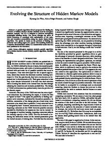
Figure 1. Comparison of label arrays obtained from several statistical models for wavelet coefficients. Top: example normalized reflectance. Second: Corresponding state label matrix from a 2-state GMM NHMC model. Third: Corresponding state label matrix from a 6-state GMM NHMC model. Bottom: Corresponding state label matrix from a MOG NHMC model with k = 6. All state labels are added with signs of corresponding wavelet coefficients.

distributions. We denote this modified model mixture of Gaussians (MOG) NHMC in the sequel. Note that we use numbers here instead of letters for the state labels to distinguish between the 2-state GMM NHMC and the 2-state MOG NHMC. In order to obtain a MOG NHMC model, the first step is to train a k-state GMM NHMC model that yields state labels Ss ∈ {0, . . . , k − 1}. After that, all the states are quantized into two states so that we can get a MOG NHMC that yields state labels Zs ∈ {0, 1} with probabilities qi,s = P (Zs = i), i = 0, 1. We provide an example comparison between labels obtained from the GMM and the MOG NHMCs in Fig. 1.

3.5. Illustration of Extracted Semantic Information The state label arrays obtained from the NHMC model characterize four important semantic features of the corresponding hyperspectral signatures: (i) the orientations of the signature slope, which is reflected in the state label values; (ii) the extent of the signature slope, which is reflected in the duration of corresponding state label values through different wavelengths; (iii) the intensity of the signature slope, which is reflected on the depth of the corresponding state label values through the scales; and (iv) the locations of the absorption bands. In order to showcase the semantic information captured by our designed features, we illustrate these four types of semantic features in several example reflectance spectra. To begin, we calculate the mean of each column in a state label array and then transform it to an integer by using round. In this way, we obtain what we call a state label mean vector of the same length as the corresponding reflectance spectrum whose possible element values are 0, ±1, · · · , ±(k−1), where k is the number of Gaus-

Figure 2. Semantic information extracted in some sample spectral curves based on GMM with 2 states. Top row: Sample spectral curves with extracted semantic information. Bottom row: corresponding state label array.

sian states used in the corresponding GMM. Fig. 2 shows three example reflectance spectra with the corresponding extracted semantic information based on an NHMC with 2 Gaussian states as well as the corresponding state label arrays. We plot the reflectance spectral curve by using three different colors to encode the value of the state label mean vector: green, red, and blue portions represent wavelengths for which the state label mean vector elements are 0, +1, and −1, respectively. Finally, we calculate all the middle points between the end of a 1’s series and the beginning of a −1’s series, and mark those points on the plotted reflectance spectra to find the locations of absorption bands. As expected, spectral curves in Fig. 2 have blue increasing slopes, red decreasing slopes, and green flat regions.

4. Experiment and Result Analysis In this section, we present multiple experimental results that evaluate the proposed concept of universality for the feature design scheme proposed in the previous section. We will consider a family of spectrum classification problems to evaluate universality by comparing the performance of features designed with a training set specific to each individual problem versus features designed with all available data being used in the training set.

4.1. Classification System Overview We provide an overview of the NHMC-based hyperspectral classification system in Fig. 3. The system consists of two modules: an NHMC model training module and a performance testing module. For illustration convenience, the figure shows an example of a binary-state GMM in the NHMC, which is the simplest model in all NHMC models proposed in this paper. We also explore the performance of

Figure 3. System overview. Top: The NHMC Training Module collects a set of training spectra, computes UWT coefficients for each, and feeds then to a NHMC training unit that outputs Markov model parameters and state labels for each of the training spectra, to be used as classification features. Bottom: The Performance Testing Module considers a test spectrum, obtains its UWT coefficients, and generates a state array from the NHMC obtained during training. A nearest-neighbors classifier searches for the most similar state array among the training data, and returns the class label for the corresponding spectrum.

the system for k-ary states extensions, k = 2, 3, . . ., as well as MOG. The training stage uses a training library of spectra containing samples from the classes of interest to train the NHMC model, which is then used to compute state estimates for each of the training spectra using a Viterbi Algorithm. The state arrays will then be used as classification features coupled with a nearest neighbor (NN) classifier. As for the similarity metric used in NN classifier, we use cosine similarity, Euclidean distance, and Manhattan distance. The testing module considers a spectrum under test and computes the state estimates under the trained NHMC model using the parameters obtained during training. The module then applies the classification scheme being tested, returning the class label of the selected training spectrum.

4.2. Study Data The dataset used in this paper is a part of the RELAB spectral database with 26 mineral reflectance spectrum classes. Since the spectra in the original database have different wavelength ranges, we only use the spectral region from 0.35 µm to 2.6 µm (if applicable) which contains almost all of the visible and near-infrared region of the electromagnetic spectrum. We only use the spectra with spectral resolution being 5 nm to eliminate the differences in spectral resolution in different sources. A different number of samples is present in each mineral class. Thus, in order to ensure the same weight of each class in the training process, we use the Hapke mixing model [8] to generate additional mixtures of existing spectra in a given class until all classes have the same number of samples. We do this to prevent different mineral types from having different contributions to the model obtained and influencing the final classification

accuracy. The final dataset contains 1690 reflectance spectra with each class including 65 reflectance spectra. Additionally, we eliminate the influences caused by illumination conditions by performing normalization on each spectrum by its maximum value. Unfortunately, the resulting dataset features a significant separation between the different classes, and so it is difficult to differentiate the performances of the different proposed methods, which are very high. In order to discriminate among the methods, we introduced mixing into the database as an attempt to increase the variance among reflectance spectra in each given class. Our mixing methodology is designed to resemble the image blurring process common in hyperspectral imaging. First, we randomly order the reflectance spectra in the database into a 3-D array (a so-called datacube) with two spatial dimensions and one spectral dimension. We then perform identical spatial blurring on each wavelength using a 3 × 3-pixel Gaussian smoothing operator. Finally, we build a new library from the blurred pixels’ spectra while retaining the original labels. By performing this image-based blurring, each spectrum in the resulting database exhibits a mixture of structural features from spectra in multiple classes, which provides a more challenging spectrum classification setup. We vary the Gaussian blurring kernel variance among a range of values to adjust the amount of mixing performed: the dominant material percentage (DMP) of the original pixel in the corresponding blurred pixel is obtained as the normalized weight of the central element in a Gaussian smoothing operator. In our experiment, we vary the DMP from 50% to 100% with a step of 5%.

4.3. Performance Evaluation We evaluate the universality of our proposed features based on the classification performance of different subsets of the whole database with NN classification coupled with different similarity metrics. We also evaluate the universality of several popular approaches for data-dependent feature selection. In this experiment, we construct new databases for classification problems by randomly selecting 7 classes, 13 classes, and 20 classes of mineral spectra from the original 26-class database with different values of DMP for the purpose of universality capability evaluation. For each DMP value, we obtain databases for 10 separate combinations of each 7-class, 13-class, and 20-class case. We randomly separate each newly built database into a training library and a validation set. The spectrum number ratio of each pair of training library and validation set is 4 : 1. We provide two hyperspectral classification schemes. In Scheme A, the features are obtained from a data-dependent feature design scheme trained on the specific classes involved in this classification problem, while in scheme B the features are obtained from the same data-dependent feature design scheme trained on all 26 classes available. The classification is then performed via NN search in the space of the features obtained for the particular scheme. For each classification problem, we calculate the classification rates of both classification schemes mentioned above (A, B) with databases containing different numbers of classes. The top row of Fig. 4 shows examples for the obtained classification rates using the proposed NHMCbased feature design scheme with a 4-state MoG and added wavelet coefficient signs. Since the results are similar for the three choices of similarity functions proposed, we show the results only for Euclidean distance for brevity. Each DMP value corresponds to 10 experiments. In some cases the figures appear to show less than 10 results for a DMP value, especially when training set is small. This is due to multiple experiments exhibiting the same classification rates under each one of the classification schemes (A,B) given above, which makes several points overlap with one another in the figure. Through the results in the top row of Fig. 4, we can find that in most cases the markers are slightly above but quite close to the y = x line. For low DMP values, more markers deviate from the y = x line than for higher DMP values. As the DMP value increases, the positions of those markers get stabilized and come closer to the y = x line. Furthermore, Scheme B seems to be more competitive when training set is small. The mixing process introduces uncertainties into the results of classification due to the fact that mixing is randomly performed in this experiment; thus, features from other spectra will be randomly added to the target spectrum. Intuitively, mixing with smaller DMP values result in larger uncertaintities in classification performance. This behavior

justifies the more diverse distribution of markers for low DMP values. The marker spread in the case of 7-class databases is the most diverse, while that of the case of 20-class databases has the strongest convergence. This may due to the fact that the difference between the feature design training databases used in schemes A and B becomes smaller as the number of classes included in the classification problem increases. In contrast, for classification problems with small number of classes, the difference between the feature design training databases used in both schemes is significant.

4.4. Comparison with Existing Data-Dependent Feature Design Approaches We compare the universality results of our proposed feature design approach with two approaches from the literature: principal component analysis (PCA) and independent component analysis (ICA) based on the infomax criterion [1]. After performing PCA on hyperspectral data, we selected the first 10 principal components of each spectrum as classification features since the first 10 principal components cover over 99% of the power in each reflectance spectrum. For Infomax-based ICA, we separated the hyperspectra data into 9 source components since we mix each reflectance spectrum with its 8 nearest neighbors in the database, which means there are totally 9 sources/endmembers contributing to a mixed spectrum. We then used the 9 source components as classification features. We still used the two hyperspectral classification schemes mentioned above (A, B) to evaluate the universality performance of the two feature-selection-based classification approaches. The second and third rows of Fig. 4 show the results of PCA and ICA, respectively. The classification results for PCA-based feature selection show quite diverse performance with regard to the different numbers of classes involved in each classification problem. This may be due to a varying level of accuracy for the subspace data model underlying the PCA approach as the data involves more classes and becomes more diverse. Furthermore, all experiments show a significant gap between the performance of schemes (A,B) due to the significant difference in modeling quality for PCA when trained with local vs. global data, which implies the lack of universality of PCA-designed features. As for the results of Infomax-based ICA, the overall classification rates of Scheme A is obviously better than that of Scheme B. This implies that features in this experiment do not contain comprehensive information for the dataset.

5. Conclusions and Further Work Our experimental results aim to show the performance gap between universal data training and problem-specific data training for several different feature design methods.

96 DMP=50% DMP=55% DMP=60% DMP=65% DMP=70% DMP=75% DMP=80% DMP=85% DMP=90% DMP=95% DMP=100%

94 92 90 88 86 84 82 80 80

85

90

95

100

92 90 88 86 84 82 85

90

95

DMP=50% DMP=55% DMP=60% DMP=65% DMP=70% DMP=75% DMP=80% DMP=85% DMP=90% DMP=95% DMP=100%

60 50 40 30 20 10 20

40

60

80

Classification Rates of Scheme B \ %

DMP=50% DMP=55% DMP=60% DMP=65% DMP=70% DMP=75% DMP=80% DMP=85% DMP=90% DMP=95% DMP=100%

70 60 50 40 30 20 10 20

40

60

80

DMP=50% DMP=55% DMP=60% DMP=65% DMP=70% DMP=75% DMP=80% DMP=85% DMP=90% DMP=95% DMP=100%

40 30 20 10 20

40

60

80

100

Classification Rates of Scheme B \ %

Classification Rates of Scheme A \ %

80

50

88 86 84 82 90

95

100

80 DMP=50% DMP=55% DMP=60% DMP=65% DMP=70% DMP=75% DMP=80% DMP=85% DMP=90% DMP=95% DMP=100%

70 60 50 40 30 20 10 0 0

20

40

60

80

100

Classification Rates of Scheme B \ % 100

90 80 DMP=50% DMP=55% DMP=60% DMP=65% DMP=70% DMP=75% DMP=80% DMP=85% DMP=90% DMP=95% DMP=100%

70 60 50 40 30 20 10 0 0

85

90

100

100

90

60

90

Classification Rates of Scheme B \ %

100

0 0

80

0 0

100

70

92

100

90

20

40

60

80

100

Classification Rates of Scheme B \ %

Classification Rates of Scheme A \ %

0 0

DMP=50% DMP=55% DMP=60% DMP=65% DMP=70% DMP=75% DMP=80% DMP=85% DMP=90% DMP=95% DMP=100%

94

Classification Rates of Scheme B \ %

Classification Rates of Scheme A \ %

80 70

96

80 80

100

100

90

Classification Rates of Scheme A \ %

Classification Rates of Scheme A \ %

DMP=50% DMP=55% DMP=60% DMP=65% DMP=70% DMP=75% DMP=80% DMP=85% DMP=90% DMP=95% DMP=100%

94

98

Classification Rates of Scheme B \ %

100

Classification Rates of Scheme A \ %

96

80 80

Classification Rates of Scheme B \ %

100

98

Classification Rates of Scheme A \ %

100

98

Classification Rates of Scheme A \ %

Classification Rates of Scheme A \ %

100

90 80 DMP=50% DMP=55% DMP=60% DMP=65% DMP=70% DMP=75% DMP=80% DMP=85% DMP=90% DMP=95% DMP=100%

70 60 50 40 30 20 10 0 0

20

40

60

80

100

Classification Rates of Scheme B \ %

Figure 4. Universality performance of several feature design schemes. We compare the classification rates for training schemes A and B over a family of classification problems with varying numbers of classes (left: 7; middle: 13; right: 20) and different feature design schemes (top: NHMC, middle: PCA, bottom: ICA). Each subfigure compares the classification performance of both schemes for a certain size of classification problems over 10 trials for each DMP value. The figures show that the NHMC features have significantly stronger universality than the alternatives presented here.

Our expectation that our feature design scheme generally had similar classification performance when trained both with problem-specific and global or generic datasets bears out in practice: the overall distribution of markers corresponding to classification results under different number of sample spectra in the object-specific training set and different amount of mixing is quite concentrated near the y = x line for the NHMC feature. Furthermore, the performance differences between these two classification schemes decreased as more classes were included in the problem, while the classification rates of each scheme decreased as the DMP was reduced. These phenomena demonstrate that our designed feature contain comprehensive signature variation in the whole database, which meets our expectation of universality. It has been previously pointed out in [18] that feature design trained with universal data may in part perform better than that trained with problem-specific data due to the fact that the dataset used in the universal case is larger (i.e., contains more data points) than the dataset used in the problem-specific case. The limited dataset sizes that

we have available prevent us from comparing feature design schemes trained from universal and problem-specific datasets of the same size, which may better quantify the universality of the feature design scheme. Additionally, we do not believe each feature designed by our method is equally significant. Conceptually, an important feature is one that is able to cause large change in classification performance; for example, [17] proposes a scheme to measure the importance of features. Thus, further work will focus on the selection of important features, which will reduce the amount of relevant data.

6. Acknowledgement We thank the faculty from the the NASA RELAB facility at Brown University for acquiring and making available the datasets used in this paper. This work was supported by the National Science Foundation under grant number IIS1319585.

References [1] A. J. Bell and T. J. Sejnowski. An information-maximization approach to blind separation and blind deconvolution. Neural Computation, 7(6):1129–1159, 1995. [2] G. Camps-Valls, D. Tuia, L. Bruzzone, and J. Atli Benediktsson. Advances in hyperspectral image classification: Earth monitoring with statistical learning methods. IEEE Signal Proc. Mag., 31(1):45–54, Jan. 2014. [3] R. Clark, G. A. Swayze, K. Livo, S. Sutley, J. Dalton, R. McDougal, and C. Gent. Imaging spectroscopy: Search and planetary remote sensing with the USGS Tetracorder and expert systems. J. Geophysical Research, 108(E12), Dec. 2003. [4] M. Crouse, R. Nowak, and R. Baraniuk. Wavelet-based statistical signal processing using hidden Markov models. IEEE Trans. Signal Proc., 46(4):886–902, Apr. 1998. [5] M. F. Duarte and M. Parente. Non-homogeneous hidden Markov chain models for wavelet-based hyperspectral image. In Allerton Conf. Communication, Control, and Computing, pages 154–159, Monticello, IL, Oct. 2013. [6] S. Feng, Y. Itoh, M. Parente, and M. F. Duarte. Tailoring non-homogeneous Markov chain wavelet models for hyperspectral signature classification. In IEEE Int. Conf. Image Proc. (ICIP), pages 5073–5077, Paris, France, Oct. 2014. [7] S. Feng, Y. Itoh, M. Parente, and M. F. Duarte. Waveletbased semantic features for hyperspectral signature discrimination. Mar. 2015. Preprint. [8] B. Hapke. Theory of reflectance and emittance spectroscopy. Cambridge University Press, 2012. [9] S. Mallat. A wavelet tour of signal processing. Academic Press, San Diego, CA, 1999. [10] S. Mallat and W. Hwang. Singularity detection and processing with wavelets. IEEE Trans. Info. Theory, 38(2):617–643, Mar. 1992. [11] S. Mallat and S. Zhong. Characterization of signals from multiscale edges. IEEE Trans. Pattern Analysis and Machine Intelligence, 14(7):710–732, Jul. 1992. [12] M. T. Orchard and K. Ramchandran. An investigation of wavelet-based image coding using an engropy-constrained quantization framework. In Data Compression Conf. (DCC), pages 341–350, Snowbird, UT, Mar. 1994. [13] M. Parente and M. F. Duarte. A new semantic wavelet-based spectral representation. In IEEE Workshop on Hyperspectral Image and Signal Proc.: Evolution in Remote Sensing (WHISPERS), Gainesville, FL, June 2013. [14] L. R. Rabiner. A tutorial on hidden Markov models and selected applications in speech recognition. Proc. IEEE, 77(2):257–285, Feb. 1989. [15] B. Rivard, J. Feng, A. Gallie, and A. Sanchez-Azofeifa. Continuous wavelets for the improved use of spectral libraries and hyperspectral data. Remote Sensing of Environment, 112:2850–2862, 2008. [16] C. Rodarmel and J. Shan. Principal component analysis for hyperspectral image classification. Surveying and Land Info. Sci., 62(2):115–122, 2002. [17] P. A. Rodriguez, N. Drenkow, D. DeMenthon, Z. Koterba, K. Kauffman, D. Cornish, B. Paulhamus, and R. J. Vogelstein. Selection of universal features for image classification. In IEEE Winter Conf. Applications of Computer Vision (WACV), pages 355–362, Steamboat Springs, CO, Mar.

2014. [18] T. Serre, L. Wolf, S. Bileschi, M. Riesenhuber, and T. Poggio. Robust object recognition with cortex-like mechanisms. IEEE Trans. Pattern Analysis and Machine Intelligence, 29(3):411–426, Mar. 2007. [19] C. Wang, M. Menenti, and Z.-L. Li. Modified principal component analysis (MPCA) for feature selection of hyperspectral imagery. In IEEE Int. Geoscience and Remote Sensing Symposium (IGARSS), volume 6, pages 3781–3783, Toulouse, France, July 2003. IEEE. [20] J. Wang and C.-I. Chang. Independent component analysisbased dimensionality reduction with applications in hyperspectral image analysis. IEEE Trans. Geoscience and Remote Sensing, 44(6):1586–1600, June 2006.