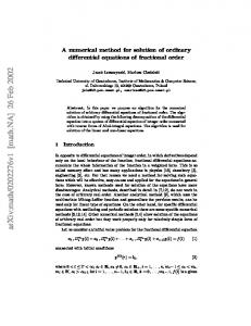
Fig.1: Solution of ODEs and PDEs via GA plus NM. Initial or Boundary Value. Problems of an ODE or a PDE. Discretization using finite differences, discretization ...
Proceedings of the 6th WSEAS Int. Conf. on Systems Theory & Scientific Computation, Elounda, Greece, August 21-23, 2006 (pp1-6)
Unstable Ordinary Differential Equations: Solution via Genetic Algorithms and the method of Nelder-Mead Nikos E. Mastorakis (*) WSEAS (Research and Development Department) http://www.worldses.org/research/index.html Agiou Ioannou Theologou 17-23 15773, Zografou, Athens, GREECE, www.wseas.org Abstract: - In this paper, a new method for solving unstable differential ordinary equations is proposed using a computational scheme of Evolutionary Computing (Genetic Algorithms) and the Nelder-Mead method. Key-Words: - Unstable Differential equations, genetic algorithms, numerical solutions
1 Introduction The numerical behavior of the unstable (ordinary) differential equations is a challenging problem especially when the differential equation is nonlinear. Most of the numerical methods (one-step or multi-step, [9]) seem to have various computational problems in the case of unstable (differential equations. This paper proposes a new methodology based on Genetic Algorithms (GA’s) and NM (Nelder-Mead Method). In [1], the author gave some ideas for the solution of the problem. It seems that the proposed methodology of [1] is good in a variety of ordinary differential equations (unstable differential equations, delay differential equations, differencedifferential equations, integro-differential equations, etc…). In many cases also the computational solution is very far from the real solution or the computational solution is absolutely impossible.
Initial or Boundary Value Problems of an ODE or a PDE
Variational Formulation (Method Rayleigh-Ritz)
Algebraic Equation or Systems of Algebraic Equations
In [1], we pointed out that we can transform the Initial Value Problems and the Boundary Value Problems to appropriate minimization problems. This minimization problems can be solved by GAs and NM as we have shown in [2]. According to [1], the initial or Boundary Value Problems of an ODE or a PDE can be transformed as follows: . 1st method: Following the particular variational principle we have the equivalent minimization problem that can be solved numerically
(*) also with: Military Institutes of University Education (ASEI), Hellenic Naval Academy, Terma Hatzikyriakou 18539, Piraeus, GREECE
Discretization using finite differences, discretization using finite elements
MINIMIZATION PROBLEM
GENETIC ALGORITHM + NELDER-MEAD Fig.1: Solution of ODEs and PDEs via GA plus NM
Proceedings of the 6th WSEAS Int. Conf. on Systems Theory & Scientific Computation, Elounda, Greece, August 21-23, 2006 (pp1-6)
2nd Method: . The finite differences or the finite elements give us an algebraic equation or a system of algebraic equations. In the Finite Elements method, we refer to the Collocation Method or the Galerkin method. These algebraic equations can be transformed to an equivalent minimization problem . (See Fig.1 as well as [1]) 3rd Method: . The finite differences or the finite elements can be formulated directly as least squares methods which are themselves a minimization problem. (See Fig.1 as well as [1])
2 Problem Formulation and Solution Before proceeding in the solution of the problem, some background on GA (Genetic Algorithms) and NM (Nelder-Mead) is necessary. In [15], the author has also proposed a hybrid method that includes a) GA (Genetic Algorithm) for finding rather the neiborhood of the global minimum than the global minimu itself and b) NM (Nelder-Mead) algorithm to find the exact point of the global minimum itself. So, with this Hybrid method of Genetic Algorithm + Nelder-Mead we combine the advantages of both methods, that are a) the convergence to the global minimum (genetic algorithm) plus b) the high accuracy of the NelderMead method. If we use only a Genetic Algorithm then we have the problem of low accuracy. If we use only NelderMead, then we have the problem of the possible convergence to a local (not to the global) minimum. These disadvantages are removed in the case of our Hybrid method that combines Genetic Algorithm with Nelder-Mead method. See [5]. We recall the following definitions from the Genetic Algorithms literature: Fitness function is the objective function we want to minimize. Population size specifies how many individuals there are in each generation. We can use various Fitness Scaling Options (rank, proportional, top, shift linear, etc…[16]), as well as various Selection Options (like Stochastic uniform, Remainder, Uniform, Roulette, Tournament)[16]. Fitness Scaling Options: We can use scaling functions. A Scaling function specifies the function that performs the scaling. A scaling function converts raw fitness scores returned by the fitness function to values in a range that is suitable for the selection function. We have the following options:
Rank Scaling Option: scales the raw scores based on the rank of each individual, rather than its score. The rank of an individual is its position in the sorted scores. The rank of the fittest individual is 1, the next fittest is 2 and so on. Rank fitness scaling removes the effect of the spread of the raw scores. Proportional Scaling Option: The Proportional Scaling makes the expectation proportional to the raw fitness score. This strategy has weaknesses when raw scores are not in a "good" range. Top Scaling Option: The Top Scaling scales the individuals with the highest fitness values equally. Shift linear Scaling Option: The shift linear scaling option scales the raw scores so that the expectation of the fittest individual is equal to a constant, which you can specify as Maximum survival rate, multiplied by the average score. We can have also option in our Reproduction in order to determine how the genetic algorithm creates children at each new generation. For example, Elite Counter specifies the number of individuals that are guaranteed to survive to the next generation. Crossover combines two individuals, or parents, to form a new individual, or child, for the next generation. Crossover fraction specifies the fraction of the next generation, other than elite individuals, that are produced by crossover. Scattered Crossover: Scattered Crossover creates a random binary vector. It then selects the genes where the vector is a 1 from the first parent, and the genes where the vector is a 0 from the second parent, and combines the genes to form the child. Mutation: Mutation makes small random changes in the individuals in the population, which provide genetic diversity and enable the GA to search a broader space. Gaussian Mutation: We call that the Mutation is Gaussian if the Mutation adds a random number to each vector entry of an individual. This random number is taken from a Gaussian distribution centered on zero. The variance of this distribution can be controlled with two parameters. The Scale parameter determines the variance at the first generation. The Shrink parameter controls how variance shrinks as generations go by. If the Shrink parameter is 0, the variance is constant. If the Shrink parameter is 1, the variance shrinks to 0 linearly as the last generation is reached.
Proceedings of the 6th WSEAS Int. Conf. on Systems Theory & Scientific Computation, Elounda, Greece, August 21-23, 2006 (pp1-6)
Migration is the movement of individuals between subpopulations (the best individuals from one subpopulation replace the worst individuals in another subpopulation). We can control how migration occurs by the following three parameters. Direction of Migration: Migration can take place in one direction or two. In the so-called “Forward migration” the nth subpopulation migrates into the (n+1)'th subpopulation. while in the so-called “Both directions Migration”, the nth subpopulation migrates into both the (n-1)th and the (n+1)th subpopulation. Migration wraps at the ends of the subpopulations. That is, the last subpopulation migrates into the first, and the first may migrate into the last. To prevent wrapping, specify a subpopulation of size zero.
Fraction of Migration is the number of the individuals that we move between the subpopulations. So, Fraction of Migration is the fraction of the smaller of the two subpopulations that moves. If individuals migrate from a subpopulation of 50 individuals into a population of 100 individuals and Fraction is 0.1, 5 individuals (0.1 * 50) migrate. Individuals that migrate from one subpopulation to another are copied. They are not removed from the source subpopulation. Interval of Migration counts how many generations pass between migrations. The Nelder-Mead simplex algorithm appeared in 1965 and is now one of the most widely used methods for nonlinear unconstrained optimization [5]÷[8]. The Nelder-Mead method attempts to minimize a scalar-valued nonlinear function of n real variables using only function values, without any derivative information (explicit or implicit). The Nelder-Mead method thus falls in the general class of direct search methods. The method is described as follows: Let f(x) be the function for minimization. x is a vector in n real variables. We select n+1 initial points for x and we follow the steps: Step 1. Order. Order the n+1 vertices to satisfy f(x1) ≤ f(x2) ≤ … ≤ f(xn+1), using the tie-breaking rules given below. Step 2. Reflect. Compute the reflection point xr from
xr = x + ρ ( x − x n+1 ) = (1 + ρ ) x − ρxn+1 , n
where x =
∑x /n i
is the centroid of the n best
i =1
points (all vertices except for xn+1). Evaluate fr=f(xr).
If f1 ≤ fr < fn , accept the reflected point xr and terminate the iteration. Step 3. Expand. If fr < f1 , calculate the expansion point xe, x e = x + χ ( x r − x ) = x + ρχ ( x − x n +1 ) = (1 + ρχ ) x − ρχx n +1
and evaluate fe=f(xe). If fe < fr, accept xe and terminate the iteration; otherwise (if fe ≥ fr), accept xr and terminate the iteration. Step 4. Contract. If fr ≥ fn, perform a contraction between x and the better of xn+1 and xr. a. Outside. If fn ≤ fr < fn+1 (i.e. xr is strictly better than xn+1), perform an outside contraction: calculate x c = x + γ ( x r − x ) = x + γρ ( x − x n +1 ) = (1 + ργ ) x − ργx n +1
and evaluate fc = f(xc). If fc ≤ fr, accept xc and terminate the iteration; otherwise, go to step 5 (perform a shrink). b. Inside. If fr ≥ fn+1, perform an inside contraction: calculate x cc = x − γ ( x − x n +1 ) = (1 − γ ) x + γx n +1 ,
and evaluate fcc = f(xcc). If fcc < fn+1, accept xcc and terminate the iteration; otherwise, go to step 5 (perform a shrink). Step 5. Perform a shrink step. Evaluate f at the n points vi = x1 + σ (xi – x1), i = 2, … , n+1. The (unordered) vertices of the simplex at the next iteration consist of x1, v2, … , vn+1. In this paper we have to solve:
Initial Value Problem of an unstable ODE The proposed method is roughly described as follows:
•
We use discretization using finite elements
•
We obtain Algebraic Equations (2nd method in Fig.1) From them a Minimization Problem is derived Finally we solve this minimization problem using Genetic Algorithm + Nelder-Mead
• •
Proceedings of the 6th WSEAS Int. Conf. on Systems Theory & Scientific Computation, Elounda, Greece, August 21-23, 2006 (pp1-6)
N
3 Examples
min ∑ Rn2 (t ) = 0 where Rn (t ) = R(t ) t =nT n =1
Example 3.1 For the ODE:
y '' − 10 y ' − 11 y = 0 The theoretical solution is: y (t ) = C1e11t + C 2 e − t However, the boundary value problem
This minimization is achieved by using Genetic Algorithms (GA) and the method of Nelder-Mead exactly as we described previously. We can use the MATLAB software package, [8]. Our GA has the following Parameters
y '' − 10 y ' − 11 y = 0 y ( 0) = 1 y ' (0) = −1 has the solution y (t ) = e − t
Population type: Double Vector
The problem with the numerical methods (one-step, multi-step etc…) is that the accumulated errors give impulse in the “unstable” term e11t and so it is impossible to find a numerical solution that will be
Fitness scaling: Rank
Population size: 30 Creation function: Uniform
−t
an approximation of the y (t ) = e . So, we will try to solve the boundary value problem
y '' − 10 y ' − 11 y = 0 y ( 0) = 1 y ' (0) = −1 with discretization using Finite Elements in order to reduce the problem to an appropriate minimization problem where we can apply GA plus NM. We consider as a simple Finite Element:
y = a + bt + ct 2 + dt 3 + εt 4 + ft 5
Selection function: roulette Reproduction: 6 – Crossover fraction 0.8 Mutation: Gaussian – Scale 1.0, Shrink 1.0 Crossover: Scattered Migration: Both – fraction 0.2, interval: 20 Stopping criteria: 100 generation So, we obtain finally:
c = 0.4999, d = −0.1667 ε = 0.0416 f = −0.0084
Applying our initial conditions:
y (0) = 1 y ' (0) = −1
The result agrees with the theoretical result:
we find a = 1 and b = −1 Introducing the solution
y (t ) = e − t
y = 1 − t + ct 2 + dt 3 + εt 4 + ft 5
Example 3.2
to y '' − 10 y ' − 11 y = 0 we can demand
For the ODE:
y '' − 100 = 0 10 t
R(t ) = (2c + 6dt + 12εt 2 + 20 ft 3 ) − 10(−1 + 2ct + 3dt 2 + 4εt 3 + 5 The ft 4 ) theoretical solution is: y (t ) = C1e
− 11(1 − t + ct 2 + dt 3 + εt 4 + ft 5 ) = 0 at several points, for example
t = 0.1, t = 0.2, t = 0.3, t = 0.4, t = 0.5,.... So, we demand R(t ) t =nT = 0 where T=0.1 and n is positive integer,
we can have n=1,2,…,N (for example N=10) So, one must find c, d , ε , f such that
+ C 2 e −10t
However, the boundary value problem
y '' − 100 = 0 y ( 0) = 1 y ' (0) = −10 has the solution y (t ) = e −10 t The problem with the numerical methods (one-step, multi-step etc…) is that the accumulated errors give impulse in the “unstable” term e10 t and so it is impossible to find a numerical solution that will be
Proceedings of the 6th WSEAS Int. Conf. on Systems Theory & Scientific Computation, Elounda, Greece, August 21-23, 2006 (pp1-6)
an approximation of the y (t ) = e −10 t . We will proceed again with discretization using Finite Elements in order to reduce the problem to an appropriate minimization problem where we can apply GA plus NM. To this end we consider the simple Finite Element:
y = a + bt + ct 2 + dt 3 + εt 4 + ft 5 We apply our initial conditions
y (0) = 1 y ' (0) = −10 and we find a = 1 and b = −10 Introducing again the solution (as a simple finite element)
y = 1 − 10t + ct 2 + dt 3 + εt 4 + ft 5 to y '' − 100 = 0 we demand R(t ) = (2c + 6dt + 12εt 2 + 20 ft 3 ) − 100 = 0 at several points, for example
t = 0.1, t = 0.2, t = 0.3, t = 0.4, t = 0.5,.... So, we demand R(t ) t = nT = 0 where T=0.1 and n is positive integer,
we can have n=1,2,…,N (for example N=10) So, we must find c, d , ε , f such that N
min ∑ Rn2 (t ) = 0 where Rn (t ) = R(t ) t =nT n =1
In every minimization step, the minimization is achieved by using Genetic Algorithms (GA) and the method of Nelder-Mead exactly as we described previously. We can use the MATLAB software package, [8]. Our GA has also the following Parameters Population type: Double Vector Population size: 30 Creation function: Uniform Fitness scaling: Rank Selection function: roulette Reproduction: 6 – Crossover fraction 0.8 Mutation: Gaussian – Scale 1.0, Shrink 1.0 Crossover: Scattered Migration: Both – fraction 0.2, interval: 20 Stopping criteria: 100 generation We obtain finally:
c = 50.0002, d = −166.6666 ε = 416.6632 f = −833.3333 The result agrees with the theoretical result:
y (t ) = e −10t
4 Conclusion In this paper, we investigated initial value problems of unstable differential equations where the classic numerical methods (one-step (like Runge-Kutta), multi-step (like Milne-Simpson, Adams-BashforthMoulton)), [9], does not give satisfactory results. Summarizing the method of this paper we can say that first of all we use discretization using finite elements and then we obtain Algebraic Equations. From these Algebraic Equations we construct a Minimization Problem which is solved using Genetic Algorithm + Nelder-Mead. Other recent relevant studies can be found in [10], [11], [12].
References:
[1] Nikos E. Mastorakis, “Solving Differential Equations via Genetic Algorithms”, Proceedings of the Circuits, Systems and Computers ’96 (CSC’96), Piraeus, Greece, July 15-17, 1996, 3rd Volume: Appendix, pp.733-737 [2] Nikos E. Mastorakis, “On the Solution of IllConditioned Systems of Linear and Non-Linear Equations via Genetic Algorithms (GAs) and Nelder-Mead Simplex Searchs”, Proceedings of the 6th WSEAS International Conference on Evolutionary Computing, Lisbon, Portugal, June 16-18, 2005. [3] Goldberg D.E. (1989), Genetic Algorithms in Search, Optimization and Machine Learning, Addison-Wesley, Second Edition, 1989 [4] Ralf Östermark, “Solving Irregular Econometric and Mathematical Optimization Problems with a Genetic Hybrid Algorithm”, Computational Economics, Volume 13 , Issue 2, pp. 103 - 115 , April 1999. [5] Lagarias, J.C., J. A. Reeds, M. H. Wright, and P. E. Wright, "Convergence Properties of the Nelder-Mead Simplex Method in Low Dimensions," SIAM Journal of Optimization, Vol. 9 Number 1, pp. 112-147, 1998. [6] J. A. Nelder and R. Mead, “A simplex method for function minimization”, Computer Journal, 7 , 308-313, 1965 [7] F. H. Walters, L. R. Parker, S. L. Morgan, and S. N. Deming, Sequential Simplex Optimization, CRC Press, Boca Raton, FL, 1991. [8] Matlab, Version 7.0.0, by Math Works, Natick, MA, 1994 http://www.mathworks.com [9] E. Balagusuramy, Numerical Methods, Tata McGraw Hill, New Delhi, 1999 [10] Gonos I.F., Mastorakis N.E., Swamy M.N.S.: “A Genetic Algorithm Approach to the
Proceedings of the 6th WSEAS Int. Conf. on Systems Theory & Scientific Computation, Elounda, Greece, August 21-23, 2006 (pp1-6)
Problem of Factorization of General Multidimensional Polynomials”, IEEE Transactions on Circuits and Systems I: Fundamental Theory and Applications, Part I, Vol. 50, No. 1, pp. 16-22, January 2003. Mastorakis N.E., Gonos I.F., Swamy [11] M.N.S.: “Design of 2-Dimensional Recursive Filters using Genetic Algorithms”, IEEE Transactions on Circuits and Systems I: Fundamental Theory and Applications, Part I, Vol. 50, No. 5, pp. 634-639, May 2003. Mastorakis N.E., Gonos I.F., Swamy [12] M.N.S.: “Stability of Multidimensional Systems using Genetic Algorithms”, IEEE Transactions on Circuits and Systems, Part I, Vol. 50, No. 7, pp. 962-965, July 2003.