Use of RBF neural networks for density estimation - CiteSeerX

Tomasz Walkowiak

Use of RBF neural networks for density estimation ABSTRACT The paper outlines a mixture distribution of Gaussian method for estimation the probability density function. A RBF neural network architecture for realising such estimation is proposed. Moreover, the learning algorithm is derived. The practical use of the method is illustrated by a small example of an recognition application. The aim of which is to recognise vehicles based on the acoustical signal generated by them. The proposed method is compared with the LVQ algorithm, giving much better results in the recognition application.

1.

INTRODUCTION

There are a number of neural network approaches to statistical pattern classification. In this paper an approach of the class conditional density estimation is investigated. The problem of estimating a probability density function could be divided into three classes: parametric, nonparametric and semiparametric methods. In the parametric methods a specific functional form for the density model is assumed. By contrast, the nonparametric estimation does not assume a particular functional form, but allows the form of the density to be determined entirely by the data. Such methods typically suffer from the problem that the number of parameters in the model grows with the size of the data set (i.e. the histogram or the Parzen windows). The third approach, used in this paper, the semiparametric method allows a very general class of functional forms in which the number of adaptive parameters allows to build flexible models, but where the total number of parameters in the model can be varied independently from the size of the data. Feed-forward neural networks could be regarded as semiparametric models for conditional density estimation [1]. The probability density function is very suitable for a classification task. Assuming that a probability density function for each class is given (denote it by fi(x)) optimal (minimum-errorrate) Bayes theory could be used (the Bayes theory is described in many standard textbooks, for example [1]). If there is no cost associated with being correct and all the prior probabilities (probabilities that an example is drawn from a given class) are equal, the optimal Bayes decision rule is choosing a class with largest values of probability density function: [EHORQJVWRFODVVL

DUJPD[ I

M

[ .

(1)

M

The next section describes the architecture of RBF network for density estimation and the learning algorithm. In section 3, a small recognition application of the proposed algorithm is presented. Finally, the author concludes with a discussion.

x1

x2

xd ...

D

input layer (d-neurons)

hidden layer (N-neurons) Ψi = F(x , m i , s i )

D

D1

output neuron

f=

N

∑ a i Ψi

i =1

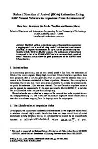
Figure 1. The RBF network for density estimation 2.

RBF NETWORK FOR PROBABILITY DENSITY ESTIMATION

An semiparametric method of a probability density function estimation called a mixture distribution is presented in this paper. Assume, that an unknown density could be represented as a linear combination of component densities F(x,θi): f (x ) =

N

∑ a i F( x , θ i ) ,

(2)

i =1

where ai presents the prior probability of the data having been generated from component i of the mixture. These priors must satisfy the constrains: N

∑ai

= 1,

0 ≤ a i ≤ 1.

i =1

(3)

The posterior probabilities could be introduced, which can be expressed using Bayes theorem: a F(x , θ i ) p( i, x ) = i . (4) f (x ) The value of p(i,x) represents the probability that a particular component i was responsible for generating the data point x. The component densities F(x,θi) could be selected from any density function. However, the attention will be limited here to the Gaussian distribution function. Moreover, the covariance matrix of the Gaussian function is assumed to be a diagonal one (a matrix having a non-zero values only on its diagonal), so that Σ=diag(s1, s2,..., sd) and hence: 2  d  x − mj  i  F(x , θ i ) = F(x , m i , s i ) = exp −0.5 ∑  . d j    j d/ 2 j =1 s i    ( 2π ) ∏ s i  

1

(5)

j=1



5%)QHXUDOQHWZRUN

Based on equations (2) and (5) a feed-forward neural network presented in Fig. 1. could be defined. The number of neurons in input layer is set equal to a dimension of example vector

(denote here as d). Each neuron from input layer is connected with each of N neurons in hidden layer. With each hidden neuron a centre vector mi and a width vector si is associated. The activation of the each hidden hidden neuron is defined by equations (5). All hidden neurons activation are multiplied by weights ai and summed giving an output from the network. This network has been named RBF, since its architecture is very similar to the RBF network proposed by Powell in >@ 7KH FDOVVLILFDWLRQ WDVN UHTXLUHV D VHSDUDWH 5%) QHWZRUN IRU HDFK FODVV DQG DGGLGWLRQDO ´ZLQHUV WDNH DOO´ OD\HU 7KLV GHFLVLRQ  OD\HU FODVVLILHV WKH SUHVHQWHG H[DPSODU EDVHG RQ %D\HV WKHRUPDFFRUGLQJWRHTXDWLRQ 7KHSURFHVVRIOHDUQLQJLVGRQHVHSDUDWO\IRUHDFKFODVV DQG LWVFRUHVSRQGLQJ5%)GHQVLW\HVWLPDWRU

2.2.

Maximum likelihood

There has been various procedures for determining the parameters of the Gaussian mixture model from a set of data. One of such methods is a maximum likelihood one. The parameter values ai, mi, si could be found by minimising the negative log-likelihood of the samples: K

E = − ln L = − ∑ ln f (x i ) ,

(6)

k =l

which can be regarded as an error function (where K is a number of training data points). Taking into consideration the constraints (4) and the error function (6), the parameter values could be found using the method of Lagrange multipliers: N  EL = E + λ  ∑ a i − 1 . (7)  i =1  Taking the partial derivative with respect to ai, setting it equal to zero, multiplying with ai, and using (4) gives: ai =

1 K ∑ p( i, x k ) . λ k =1

(8)

Summing (8) across i and using (2)-(4), we get λ=K. Similarly, other parameter values could be found: K

K

∑ p(i, x k )( x k − m i ) 2

∑ p( i, x k ) x k

m i = k =1

K

∑ p ( i, x k )

k =1

2.3.

,

j ( si ) 2 = k = 1

j

K

j

.

(9),(10)

∑ p( i, x k )

k =1

Initial values

Very important in learning of neural networks and almost in all tasks of searching a global minimum is selecting a starting point of a search. A good initial value could result in fast convergence of the algorithm and hopefully will prevent from dropping into local minimum. This is not a trivial task, but the RBF neural network has a good interpretation of its weights (parameter values of a model) and a simple algorithm of selecting initial values could be easily derived. In the first step, centers mi are assigned using the k-means clustering algorithm [3]. Next, the width parameters si are estimated. Initially, each of the hidden neurons has associated with it a single scalar width parameter σi. These widths are found using the following P-nearest neighbour heuristic. The width of any hidden neuron (σi) is taken as the root mean square distance to the P nearest centres:





σi =

mi − mp

P

∑

2 

P

p =1



The next step is to adapt the hidden neurons to the local character of the data. The width parameters si are calculated based on the training points “captured” by each hidden neuron. To determine which training points are “captured” by a particular neuron the following weight function is used: 

w i (x k ) = exp( − x k − m i

2

/ σ 2i ) 



The weight for point xk in neuron i is wi(xk). The weighting function is used instead of a hard or crisp boundary because such hard boundaries imply a threshold value that would have to be set arbitrarily. Using the continuos membership function, the points that are near the neuron centre have a significant influence on the shape of the neuron, while points far away from the centre have a small effect on the shape. Width parameters for a particular neuron i (si) based on a weighted data are given by a formula: K

∑ w i (x k )( x k − m i ) 2

j ( si ) 2 = k = 1

j

j



K



∑ w i (x k )

k =1

After the centres and widths are calculated, the next task is to determine parameters ai for weights from hidden neurons to the output neuron. These parameters represent a probability that a particular neuron i is responsible for generating a data point. It could be estimated as a number of effective points associated with a neuron i (defined it by ni) divided by a total number of points: ni ai = . (14) N

∑nj

j= 1

The number of effective points associated with a neuron i is calculated as a sum of the activationF(x,θi) of each data point xk for a given neuron L ni = 2.4.

K

∑ F( x k , m i , s i )





k =1

Learning algorithm

Equations (8),(9) and (10) give a method of a recursive updating parameter values of mi, si , ai. This minimises the log-likelihood error. Therefore, a learning algorithm of an RBF network could be defined as follows: 1. Initialise the values of mi, si , ai according to the initialisation algorithm defined in section 2.3. 2. Using actual values of mi, si , ai calculate posterior probabilities p(i,xk) for all data points xk and all hidden neurons using equations (2),(4) and (5).

3. Set a previous global error Eold equal to previous value of Enew . Next, calculate a new global log-likelihood error Enew as defined in (6).  ,IDEVEnew - Eold )/Enew ) < ε stop, otherwise continue. 5. Calculate new parameter values using posterior probabilities p(i,xk) calculated in step 2: a) new value of centres mi according to equation (9), b) new value of widths si according to equation (10) using new values of centres mi from previous substep, c) new prior probabilities ai are given by equation (8). 6. Go to step 2. It should be stated here that the above algorithm is very similar (steps 2 and 5) to the EM algorithm proposed in [4]. 2.5.

Implementation notes

As it was mentioned in section 2.4, an initial selection of parameter values is crucial for the algorithm. The most important part is a selection of initial values for centres mi. The k-means clustering algorithm, used here, is not the best solution, since it gets stuck into local minimum. Therefore, the k-means clustering algorithm is run several times and the solution with the smallest distortion value is selected as an initial value of centres. Other problem is connected with calculation of log-likelihood (6), since the logarithm of a possible very small value of density function f(xk) could result in the minus infinity output. Moreover, an iterative procedures of (8), (9) and (10) may cause a singular solution with a component density (neuron) centred on a single design sample. In such situation the prior probabilities ai goes to zero and width values si to infinity. To prevent such situation the values of aiF(xk,θi) in equations (2) and (4) are bounded. They can not exceed some large predefined value and cannot be smaller then some other small predefined value 3.

PRELIMINARY EXPERIMENTS

The proposed algorithm has been tested in a small recognition application. In this case the task was to recognise the four different military vehicles (BWP, MTLB, SKOT and T-72) based on the acoustical signal generated by them. The recorded acoustical signal has been digitised at frequency of 5 kHz. Next, the raw date has been filtered throughout a bank filter. The bank filter consists of 8 channels, spanning from 100 to 2500 Hz. Each filter in the filter bank is sensitive to a narrow band of a frequency, equally spaced on a logarithmic scale (exactly the Greenwood proposition of the human ear basilar membrane frequency-position function [5] has been used). Next, a square root of a energy is calculated by summing the 0.5 sec part of the rectified output signal from filters. Finally, the 8 values of energy from each filter are normalised. These values are divided by the total energy of each 0.5 fragment of the signal. This preprocessing results in a 8 dimensional sample space. Detailed information concerning the data collection and the preprocessing could be found in [6]. Each of four classes is represented by a separate RBF network (each one consisted of 5 hidden neurons). The achieved results of recognition for the training and testing set are presented in Tab. 1. Moreover, the LVQ algorithm [7] with 40 neurons has been used for the same classification task and the results are also presented in Tab. 1.

Type of the object BWP MTLB SKOT T-72

RBF train test 88.44% 88.44% 79.22% 78.42% 88.11% 88.11% 89.63% 88.15%

LVQ train test 65.31% 64.56% 56.43% 56.02% 77.84% 77.30% 90.37% 90.00%

Table 1. Classification results (percent of correct recognition) 4.

DISCUSSION

The proposed algorithm outperforms the LVQ algorithm in the exemplar experiment as it could be seen in Tab. 1. Moreover, it has an advantage over classification algorithms based on minimising some misclassification error function (like for example the multilayer perceptron), that the proposed algorithm could be easily extended to a new class of samples. In the proposed algorithm each class is learned separately and adding a new class does not require learning of all network, only a new class probability density function must be estimated. Additionally, except a classification answer the network could give a probability answer, stating the probability of the example belonging to each class. The other important feature of this algorithm is its easy extension to the detection problem, when classification is based not on a simple example by on a set of examples. In such case, assuming that the examples are independent in the probability sense, the value of probability density function is given by the product of the density functions of each example in the set. It is obvious that the proposed algorithm is not free of problems. The initial selection of centres is crucial to this algorithm and requires the further investigation. Achieving a good estimation of probability density function, and therefore according to Bayes theory an optimal classification results, requires a large date representation of each class. The number of hidden neurons (like in other neural networks) is a free parameter, which choice is important for the final performance of the network. And of course the simple testing exemplar does not tell much about the algorithm performance with comparison to other classification methods. REFERENCES [1] Ch. M. Bishop, “Neural Networks for Pattern Recognition”, Clarendon Press, Oxford, 1995. [2] M. J. D. Powell, “Radial basis functions for multivariable interpolation: a review”, J.C.Mason and M.G. Cox (Eds.) Algorithms for Approximation, Clarendon Press, Oxford, pp. 143-167, 1987. [3] J. MacQueen, “Some Methods for Classification and Analysis of Multivariative Observations”, Proc. Fith Berkeley Symp. Math. Stat. and Prob., Berkeley, vol. I, pp. 281-297, 1967. [4] A. P. Dempster, N. M. Laird, D. B. Rubin, “ Maximum likelihood from incomplete data via the EM algorithm”, Journal of Royal Statistical Society, vol. B 39, pp. 1-38, 1977. [5] D. D. Greenwood, “A cohlear frequency-position function for several species- 29 years later”, J. Acoust. Soc. Am., vol. 87, pp. 2592-2605, 1990. [6] W. Zamojski, J. Jarnicki, H. Maciejewski, J. Mazurkiewicz, T. Walkowiak, “System ropoznanwania i detekcji ruchu obiektu”, I Konferencja Granty-Automatyka, PIAP, Warszawa, 27-29.VI.1995. [7] T. Kohonen, “Self-Organisation and Associative Memory”, Springer, Berlin-HeidelbergNew York-Tokyo, 1988.