Pruning Neural Networks with Distribution Estimation Algorithms Erick Cant´ u-Paz Center for Applied Scientific Computing Lawrence Livermore National Laboratory Livermore, CA 94551
[email protected]
Abstract. This paper describes the application of four evolutionary algorithms to the pruning of neural networks used in classification problems. Besides of a simple genetic algorithm (GA), the paper considers three distribution estimation algorithms (DEAs): a compact GA, an extended compact GA, and the Bayesian Optimization Algorithm. The objective is to determine if the DEAs present advantages over the simple GA in terms of accuracy or speed in this problem. The experiments considered a feedforward neural network trained with standard backpropagation and 15 public-domain and artificial data sets. In most cases, the pruned networks seemed to have better or equal accuracy than the original fully-connected networks. We found few differences in the accuracy of the networks pruned by the four EAs, but found large differences in the execution time. The results suggest that a simple GA with a small population might be the best algorithm for pruning networks on the data sets we tested.
1
Introduction
The success of neural networks (NNs) largely depends on their architecture, which is usually determined by a trial-and-error process. Evolutionary algorithms (EAs) have been used in numerous ways to optimize the network architecture to reach the highest possible classification accuracy [1, 2]. In the present paper, we examine neural network pruning by four evolutionary algorithms to improve the generalization accuracy in classification problems. We experimented with a simple genetic algorithm (sGA) and three distribution estimation algorithms (DEAs): a compact GA (cGA), an extended compact GA (ecGA), and the Bayesian Optimization Algorithm (BOA). Instead of the mutation and crossover operations of conventional GAs, DEAs use a statistical model of the individuals that survive selection to generate new individuals. Numerous experimental and theoretical results show that DEAs can solve hard problems reliably and efficiently [3–5]. The objective of this study is to determine if DEAs present advantages over simple GAs in terms of accuracy or speed when applied to neural network pruning. The experiments used conventional feedforward perceptrons with one hidden
layer and were trained with the backpropagation algorithm. The experiments used 13 public-domain and two artificial data sets. Our target was to maximize the accuracy of classification. The experiments demonstrate that, in most cases, the accuracy of the pruned networks is at least as good as that of fully-connected networks. We found few significant differences in the accuracy of networks pruned by the four EAs, but found large differences in the execution time. The next section presents background on neural network pruning, including some previous applications of EAs to this task. Section 3 describes the algorithms, data sets, and the method used to compare the algorithms. The experimental results are presented in section 4. Section 5 concludes this paper with a summary, the conclusions of this study, and a discussion of future research directions.
2
Neural Network Pruning
It is well known that a network that is too big for a particular classification task is more likely to overfit the training data and have poor performance on unseen examples (i.e., poor generalization) than a small network. Therefore, a heuristic to obtain good generalization is to use the smallest network that will learn to classify correctly the training data. However, the optimal network size is usually unknown and tedious experimentation becomes necessary to find it. An alternative to improve generalization is to train a network that is believed to be larger than necessary and prune the excess parts. Numerous algorithms have been used to prune neural networks [6]. Pruning begins by training a fully-connected neural network. Most pruning methods delete a single weight at a time in a greedy fashion, which may result in suboptimal pruning. Additionally, many pruning methods fail to account for the interactions among multiple weights. This may be problematic if deleting one weight makes it appear as if another weight that should be pruned is important for the operation of the network. An algorithm that considers weight interactions and more than one weight at a time may have a better chance of reducing the size of the network significantly without affecting the classification accuracy. For these reasons, GAs and DEAs seem promising for NN pruning. Genetic algorithms have been used to prune networks with good results [7–9]. Applying GAs to prune networks is straightforward: The chromosomes contain one bit for each weight of the original network, and the value of the bit determines whether the weight will be used in the final network. This simple binary encoding is used in the experiments in the present paper. More sophisticated methods of simultaneously training and pruning the networks were introduced by Schmidt and Stidsen [10]. Whitley [11] suggests to retrain the network for a few epochs after pruning the weights. We performed experiments to test this idea, but our experiments show only limited advantages of retraining.
It is also possible to prune entire (input and hidden) nodes, but in the present paper we experiment only with the more common approach of pruning individual weights. We leave pruning units to future work.
3
Methods
This section describes the algorithms and the data sets used in this paper as well as the statistical method used to compare the algorithms. 3.1
Algorithms
The simple genetic algorithm in this study uses binary strings, pairwise tournament selection without replacement, uniform crossover, and bitwise point mutation. Simple GAs such as this have been used successfully in many applications. However, it has long been recognized that the problem-independent crossover operators used in simple GAs can disrupt groups of related variables and prevent the algorithm from reaching the global optimum, unless exponentially-sized populations are used. (Thierens [12] gives a good description of this problem). One approach to identify and exploit the relationships among variables is to estimate the joint distribution of the individuals that survive selection and use this model to generate new individuals. The complexity of the models has increased over time as more sophisticated methods of building models from data and more powerful computers become available. Interested readers can consult the reviews by Pelikan et al. [13] and Larra˜ naga et al. [14]. The simplest model-building EA used in the experiments reported here is the compact GA [15]. This algorithm assumes that the variables (bits) that represent the problem are independent, and therefore the cGA models the population as a product of Bernoulli distributions. The compact GA receives its name from its small memory requirements: Instead of using an explicit population, the cGA uses a vector p of length equal to the problem’s length, l. Each element of p contains the probability that a sample will take the value 1. If the Bernoulli trial is not successful the sample will be 0. All positions of p are initialized to 0.5 to simulate the usual uniform random initialization of simple GAs. New individuals are obtained by sampling consecutively from each position of p and concatenating the values obtained. The probabilities vector is updated by comparing the fitness of two individuals obtained from it. For each pk , k = 1, .., l, if the fittest individual has a 1 in the k-th position, pk is increased by 1/n, where n is the size of the virtual population that the user wants to simulate. Likewise, if the fittest individual has a 0 in the k-th position, pk is decreased by 1/n. The cGA iterates until all positions in pk contain either zero or one. PBIL [16] and the UMDA [17] are other algorithms that use univariate models and operate on binary alphabets. They differ from the cGA in the method to update the probabilities vector. The extended compact GA [18] uses a product of marginal distributions on a partition of the variables. In this model, subsets of variables are modeled jointly, and the subsets are considered independent of other subsets. Formally, the model
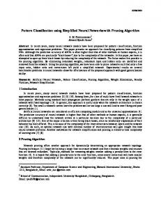
(a) ecGA
(b) BOA
Fig. 1. Representation of the models used in the ecGA and the BOA. Variables are represented as circles. The ecGA groups related variables into subsets, but cannot represent individual relationships among variables in the same subset.
Qm is P = i=0 Pi , where m is the number of subsets in a partition of the variables and Pi represents the distribution of the i-th subset. The distribution of a subset with k members is stored in a table with 2k − 1 entries. The challenge is to find a partition that models the population correctly. Harik [18] proposed a greedy search that initially supposes that all variables are independent. The model search tries to merge all pairs of subsets and chooses the merger that minimizes a complexity measure based on information theory. The search continues until no further subsets can be merged. In contrast to the cGA, the ecGA has an explicit population that is evaluated and is subject to selection at each iteration of the algorithm. The algorithm builds the model considering only those solutions that survive selection. The population is initialized randomly, and new individuals are generated by sampling consecutively from the m subset distributions. The Bayesian Optimization Algorithm [3] models the selected individuals using a Bayesian network, which can represent dependence relations among an arbitrary number of variables. Independently, Etxeberria and Larra˜ naga [4] and M¨ uhlenbein and Mahnig [5] introduced similar algorithms. The BOA uses a greedy search to optimize the Bayesian Dirichlet metric, a measure of how well the network represents the data (the BOA could use other metrics). The user specifies the maximum number of incoming edges to any node of the network. This number corresponds to the highest degree of interaction assumed among the variables of the problem. As the ecGA, the BOA builds the model considering only the solutions that survived selection. New individuals are generated by sampling from the Bayesian network. The main difference between the ecGA and the BOA is the model that they use to represent the survivors. Figure 1 illustrates the different models used by the ecGA and the BOA. The ecGA cannot represent individual relationships among the variables in a subset.
The experiments used the C++ implementations of the ecGA [19] and the BOA version 1.0 [20] that are distributed by their authors on the web (at http://www-illigal.ge.uiuc.edu). The ecGA code has a non-learning mode that emulates the cGA. The sGA and the neural network were developed in C++. All programs were compiled with g++ version 2.96 using -O2 optimizations. The experiments were executed on a single processor of a Linux (Red Had 7.2) workstation with dual 2.4 GHz Intel Xeon processors and 512 Mb of memory. The ecGA and the BOA codes were modified to use a Mersenne Twister random number generator, which was also used in the GA and the data partitioning. The algorithms used populations with 1024 individuals and were initialized uniformly at random. The GA used uniform crossover with probability 1.0, and mutation with probability 1/l, where l was the length of the chromosomes and corresponds to the total number of weights in the network. Promising solutions were selected with pairwise binary tournaments without replacement. The cGA, ecGA, and the BOA used the default parameters provided in their distributions: The cGA and ecGA used tournaments among 16 individuals, and the BOA used truncation selection with a threshold of 50%. All algorithms were terminated after observing no improvement in the best individual over five consecutive generations, or until a limit of 50 generations was reached. The network used in the experiments was a fully-connected perceptron with a single hidden layer. The hiddenPand output units compute their output as d f (net) = tanh(net), where net = i=1 xi wi + w0 is the net activation, the xi are inputs to the unit, wi are the connection weights and w0 is a bias term. The weights were initialized uniformly at random in the interval [-1,1]. Before each EA run, a fully-connected network was trained with simple backpropagation using a learning rate of 0.15 and a momentum term of 0.9. In each epoch, the examples were presented to the network in a different random order. The sizes of the network and the number of training epochs varied for each data set and are specified in table 1. For all the algorithms, the classification accuracy of the pruned network on the training data served as the fitness function. In cases where the pruned network was retrained with backpropagation, the algorithms exploited the Baldwin effect: The retrained pruned network was used to evaluate the fitness, but the retrained weights were not inherited. Note that the fitness measure does not bias the search explicitly toward networks with few weights. Adding this bias is a future extension of the work presented here. 3.2
Data Sets
The data sets used in the experiments are described in table 1. The data sets are available in the UCI machine learning repository [21], except for Random21 and Redundant21, which are artificial data sets with 21 features each. The target concept of these two data sets is whether the first nine features are closer to (0,0,...,0) or (9,9,...,9) in Euclidean distance. The features were generated uniformly at random in the range [3,6]. All the features in Random21 are random,
Table 1. Description of the data sets used in the experiments. For each data set, the table shows the number of instances; the number of classes; the number of continuous and discrete features; the number of input, hidden, and output units; and the number of epochs of backpropagation used to train the networks.
Domain Breast Cancer Credit-Australian Credit-German Heart-Cleveland Housing Ionosphere Iris Kr-vs-kp Pima-Diabetes Segmentation Sonar Vehicle Wine Random21 Redundant21
Features Neural Network Cases Class Cont. Disc. Input Output Hidden Epochs 699 2 9 – 9 1 5 20 653 2 6 9 46 1 10 35 1000 2 7 13 62 1 10 30 303 2 6 7 26 1 5 40 506 3 12 1 13 3 2 70 351 2 34 – 34 1 10 40 150 3 4 – 4 3 5 80 3196 2 – 36 74 1 15 20 768 2 8 – 8 1 5 30 2310 7 19 – 19 7 15 20 208 2 60 – 60 1 10 60 846 4 18 – 18 4 10 40 178 3 13 – 13 3 5 15 2500 2 21 – 21 1 1 100 2500 2 21 – 21 1 1 100
and the first, fifth, and ninth features are repeated four times each in Redundant21. We took the definition of Redundant21 from the paper by Inza et al. [22]. Each numeric feature in the data was linearly normalized to the interval [−1, 1]. The discrete features and the class labels were encoded with the usual 1-in-C coding if there are C > 2 values (one of the C outputs is set to 1 and the rest to -1). Binary values were encoded as a single -1 or 1 value. The instances with missing values in Credit-Australian were deleted. Following the usual practice, the missing values in Pima-Diabetes (denoted with zeroes) were not removed and were treated as if their values were meaningful. Following Lim et al. [23], the classes in Housing were obtained by discretizing the attribute “mean value of owner-occupied homes” as follows: class = 1 if log(median value) ≤ 9.84, class = 2 if 9.84 < log(median value) ≤ 10.075, and class = 3 otherwise. 3.3
Evaluation Method
To evaluate the generalization accuracy of the pruning methods, we used 5 iterations of 2-fold crossvalidation (5x2cv). In each iteration, the data were randomly divided in halves. One half was input to the EAs. The best pruned network found by the EA was tested on the other half of the data. The accuracy results presented in table 2 are the averages of the ten tests. To determine if the differences among the algorithms were statistically sig(j) nificant, we used a combined F test proposed by Alpaydin [24]. Let pi denote
Table 2. Mean accuracies found in the 5x2cv experiments. Bold typeface indicates the best result and those not significantly different from the best according to the combined F test at a 0.05 level of significance. Domain Breast Cancer Cr-Australian Cr-German Heart-Cleveland Housing Ionosphere Iris Kr-vs-kp Pima-Diabetes Segmentation Sonar Vehicle Wine Random21 Redundant21
Unpruned 96.39 82.53 70.12 58.17 64.62 84.77 94.53 74.30 73.30 44.16 73.17 69.71 95.16 91.70 91.75
sGA 96.54 85.78 70.68 89.70 75.36 84.61 92.93 92.56 74.84 64.02 83.46 78.20 94.15 94.04 95.77
cGA 96.13 85.75 70.92 88.05 67.11 82.95 70.13 93.53 75.91 62.45 86.15 76.73 89.88 94.08 95.82
ecGA 95.84 86.18 70.30 88.78 64.18 82.22 67.73 93.81 76.04 64.32 84.90 76.64 87.41 94.03 95.82
BOA 96.42 85.84 70.14 89.37 66.24 84.22 93.60 93.85 75.88 63.66 83.55 78.62 93.48 94.09 95.72
the difference in the accuracy rates of two classifiers in fold j of the i-th iteration (1) (2) (1) (2) of 5x2cv, p¯ = (pi + pi )/2 denote the mean, and s2i = (pi − p¯)2 + (pi − p¯)2 the variance, then P5 P2 ³ (j) ´2 j=1 pi i=1 f= P5 2 i=1 s2i
is approximately F distributed with 10 and 5 degrees of freedom, and we rejected the null hypothesis that the two algorithms have the same error rate with a 0.05 level of significance if f > 4.74 [24]. The algorithms used the same data partitions and started from identical initial populations.
4
Experiments
Table 2 has the average accuracies obtained with each method. For each data set, the best observed result and those that according to the combined F test are not significantly different from the best are highlighted in bold type. These results suggest that, in most cases, the accuracy of the pruned networks is at least as good as the original fully-connected networks. In these experiments the networks were not retrained after pruning. Unexpectedly, pruning does not seem to have harmful effects on the accuracy, except in two cases (Iris and Wine) where the networks pruned with cGA and ecGA perform significantly worse than the fully-connected networks. The simple GA and the BOA performed equally well, and their results were not significantly different than the best result for all the data sets we tried.
Pruning results in only minor accuracy gains over the fully-connected networks, except when the fully-connected nets performed poorly. In those cases, pruning resulted in dramatic improvements. For example, the pruned networks on Heart-Cleveland show improvements of ≈30% in accuracy, while in Kr-vs-kp and Segmentation the improvements are ≈20%, and in Vehicle the improvements are ≈10%. One reason why pruning might improve the accuracy is because pruning may eliminate the effect of irrelevant or redundant inputs. The experiments with Random21 and Redundant21 were intended to explore this hypothesis. In Random21, the pruning methods always selected weights corresponding to the nine true inputs, but the algorithms always selected two or three additional weights corresponding to random inputs. However, the performance does not seem to degrade much. It is possible that backpropagation had assigned low values to those irrelevant weights or it may be that the hypothesis that pruning improves the accuracy by removing irrelevant weights is wrong. Further work is required to clarify these results. In Redundant21, the pruning methods did not eliminate the redundant features. In fact, the pruned networks retained more than 20 of their 24 weights. Again, it is not clear why the performance did not degrade with the redundant weights and additional work is needed to address this issue. With respect to the number of weights of the final networks, all algorithms had similar results, successfully pruning between 30 and 50% of the total weights (with the exception of Redundant 21 discussed above). Table 3 shows that the sGA and the BOA finished in similar number of generations (except for Credit-Australian and Heart-Cleveland), and were the slowest algorithms in most cases. On most data sets, the ecGA finishes faster than the other algorithms.1 However, the ecGA produced networks with inferior accuracy than the other methods or the fully-connected networks in three cases (Housing, Iris, and Wine). Despite the occasional inferior accuracies, it seems that the ecGA is a good pruning method with a good compromise of accuracy and execution time. However, further experiments described below suggest that simple GAs might be the best option. We performed additional experiments retraining the networks after pruning for one, two, and five epochs of backpropagation (results not shown). In most cases, retraining the networks improves the classification accuracy only slightly over pruning without retraining (1–2%), and there does not appear to be a significant advantage to retrain for more than one epoch. Among the data sets we tested, the largest impact of retraining (using one epoch) was in Housing with an increase of approximately 7% over pruning without retraining. Retraining, however, had a large impact on the number of generations until the algorithms terminated. In most cases, retraining for one epoch reduced the generations by approximately 40%. Only in one case (sGA on Random21) the 1
The time needed by the DEAs to build a model of the selected individuals and generate new ones was short compared to the time consumed evaluating the individuals, so one generation took roughly the same time in all algorithms.
Table 3. Mean generations until termination. Bold typeface indicates the best result and those not significantly different from the best according to the combined F test at a 0.05 level of significance. Domain Breast Cancer Credit-Australian Credit-German Heart-Cleveland Housing Ionosphere Iris Kr-vs-kp Pima-Diabetes Segmentation Sonar Vehicle Wine Random21 Redundant21
sGA 9.2 10 17.1 9.8 19.4 16.8 10.1 37.7 12.8 26 14.5 26.1 12.5 13.6 13.7
cGA 6.7 14 22.8 10.4 7.4 15.7 5.9 28.8 14.7 18.1 20.5 16.5 9.9 9 8.5
ecGA 7 14.9 21.3 10.2 7.1 15.1 5.9 26 11.5 17.4 19.3 14.8 9.4 9.1 8.5
BOA 10.9 14.4 14.3 15.8 18.6 17.8 10.1 35.7 14.2 24.9 16.9 30.2 11.7 14.8 16.1
number of generations increased (from 13.6 to 20). Retraining for more than one epoch did not have a noticeable effect on the number of generations. Of course, in all cases, retraining increased the total execution time considerably. The population size of 1024 individuals was chosen because the DEAs require a large population to estimate correctly the parameters of the models of selected individuals. However, for the simple GAs, it is likely that such a large population is unnecessary. In√additional experiments, we set the sGA population size to the largest of 20 or 3 l, where l is the size of the chromosomes (number of weights in the network). The only significant difference in accuracy between the sGA with 1024 individuals and the smaller population was in Iris (87.73% with 20 individuals vs. 92.93% with 1024). There were no other significant differences with the sGA with the large population or the best pruning method for each data set. Naturally, the execution time was much shorter with the smaller populations. Therefore, for pruning neural networks, it seems that the best alternative among the algorithms we examined is a simple GA with small populations.
5
Conclusions
This paper presented experiments with four evolutionary algorithms applied to neural network pruning. The experiments considered public-domain and artificial data sets. With these data sets we found that there are few differences in the accuracy of networks pruned by the four EAs, but that the extended compact GA needs fewer generations to finish. However, we also found that, in a few cases, the ecGA results in networks with lower accuracy than those obtained by the other EAs or a fully-connected network.
We also found that in most cases retraining the pruned networks improves the classification accuracy only very slightly but incurs in a much higher computational cost. Therefore, it appears that retraining is only recommended in applications where time is not critical. Additional experiments revealed that a simple GA with a small population can reach results that are not significantly different from the best pruning methods. Since the smaller populations result in much shorter execution times, the simple GA seems to have an advantage over the other methods. The experiments with redundant and irrelevant attributes presented here are not conclusive and additional work is needed to clarify those results. Future work is also necessary to explore methods to improve the computational efficiency of the algorithms to deal with much larger data sets. In particular, subsampling the training sets and parallelizing the fitness evaluations seem like promising alternatives. Another possible extensions of this work are to prune entire units and attempt to reduce the size of the pruned networks by including a bias toward small networks in the fitness function.
Acknowledgments I thank Martin Pelikan for providing the graphs in figure 1 and the anonymous reviewers for their detailed and constructive comments. UCRL-JC-151521. This work was performed under the auspices of the U.S. Department of Energy by University of California Lawrence Livermore National Laboratory under contract No. W-7405-Eng-48.
References 1. Yao, X.: Evolving artificial neural networks. Proceedings of the IEEE 87 (1999) 1423–1447 2. Castillo, P.A., Arenas, M.G., Castillo-Valdivieso, J.J., Merelo, J.J., Prieto, A., Romero, G.: Artificial neural networks design using evolutionary algorithms. In: Proceedings of the Seventh World Conference on Soft Computing. (2002) 3. Pelikan, M., Goldberg, D.E., Cant´ u-Paz, E.: BOA: The Bayesian optimization algorithm. In Banzhaf, W., Daida, J., Eiben, A.E., Garzon, M.H., Honavar, V., Jakiela, M., Smith, R.E., eds.: Proceedings of the Genetic and Evolutionary Computation Conference 1999: Volume 1, San Francisco, CA, Morgan Kaufmann Publishers (1999) 525–532 4. Etxeberria, R., Larra˜ naga, P.: Global optimization with Bayesian networks. In: II Symposium on Artificial Intelligence (CIMAF99). (1999) 332–339 5. M¨ uhlenbein, H., Mahnig, T.: FDA-A scalable evolutionary algorithm for the optimization of additively decomposed functions. Evolutionary Computation 7 (1999) 353–376 6. Reed, R.: Pruning algorithms—a survey. IEEE Transactions on Neural Networks 4 (1993) 740–747 7. Whitley, D., Starkweather, T., Bogart, C.: Genetic algorithms and neural networks: Optimizing connections and connectivity. Parallel Computing 14 (1990) 347–361
8. Hancock, P.J.B.: Pruning neural networks by genetic algorithm. In Aleksander, I., Taylor, J., eds.: Proceedings of the 1992 International Conference on Artificial Neural Networks. Volume 2., Amsterdam, Netherlands, Elsevier Science (1992) 991–994 9. LeBaron, B.: An evolutionary bootstrap approach to neural network pruning and generalization. unpublished working paper (1997) 10. Schmidt, M., Stidsen, T.: Using GA to train NN using weight sharing, weight pruning and unit pruning. Technical report, Aarhus University, Computer Science Department, Aarhus, Denmark (1995) 11. Whitley, D., Bogart, C.: The evolution of connectivity: Pruning neural networks using genetic algorithms. Technical Report CS-89-113, Colorado State University, Department of Computer Science, Fort Collins (1989) 12. Thierens, D.: Scalability problems of simple genetic algorithms. Evolutionary Computation 7 (1999) 331–352 13. Pelikan, M., Goldberg, D.E., Lobo, F.: A survey of optimization by building and using probabilistic models. IlliGAL Report No. 99018, University of Illinois at Urbana-Champaign, Illinois Genetic Algorithms Laboratory, Urbana, IL (1999) 14. Larra˜ naga, P., Etxeberria, R., Lozano, J.A., Pe˜ na, J.M.: Optimization by learning and simulation of Bayesian and Gaussian networks. Tech Report No. EHU-KZAAIK-4/99, University of the Basque Country, Conostia-San Sebastian, Spain (1999) 15. Harik, G.R., Lobo, F.G., Goldberg, D.E.: The compact genetic algorithm. In: Proceedings of the 1998 IEEE International Conference on Evolutionary Computation, Piscataway, NJ, IEEE Service Center (1998) 523–528 16. Baluja, S.: Population-based incremental learning: A method for integrating genetic search based function optimization and competitive learning. Tech. Rep. No. CMU-CS-94-163, Carnegie Mellon University, Pittsburgh, PA (1994) 17. M¨ uhlenbein, H.: The equation for the response to selection and its use for prediction. Evolutionary Computation 5 (1998) 303–346 18. Harik, G.: Linkage learning via probabilistic modeling in the ECGA. IlliGAL Report No. 99010, University of Illinois at Urbana-Champaign, Illinois Genetic Algorithms Laboratory, Urbana, IL (1999) 19. Lobo, F.G., Harik, G.R.: Extended compact genetic algorithm in C++. IlliGAL Report No. 99016, University of Illinois at Urbana-Champaign, Illinois Genetic Algorithms Laboratory, Urbana, IL (1999) 20. Pelikan, M.: A simple implementation of the Bayesian optimization algorithm (BOA) in C++ (version 1.0). IlliGAL Report No. 99011, University of Illinois at Urbana-Champaign, Illinois Genetic Algorithms Laboratory, Urbana, IL (1999) 21. Blake, C., Merz, C.: UCI repository of machine learning databases (1998) 22. Inza, I., Larra˜ naga, P., Etxeberria, R., Sierra, B.: Feature subset selection by Bayesian networks based on optimization. Artificial Intelligence 123 (1999) 157– 184 23. Lim, T.J., Loh, W.Y., Shih, Y.S.: A comparison of prediction accuracy, complexity, and training time of thirty-three old and new classification algorithms. Machine Learning 40 (2000) 203–228 24. Alpaydin, E.: Combined 5 × 2cv F test for comparing supervised classification algorithms. Neural Computation 11 (1999) 1885–1892