Use of the non-quadratic mixing rules for prediction of VLE in polar organic binary solutions Amir Vahid, Fatemehsadat Emami, Farzaneh Feyzi
*
Thermokinetic Research Laboratory, Department of Chemical Engineering, Iran University of Science and Technology, Tehran, P.O.Box 16846, Iran,Tel:+98-21-73912727, Fax:+98-21-7896620
[email protected]
9th Iranian Chemical Engineering Congress
Iran University of Science and Technology 23-25 November, 2004
Abstract In this research, the capabilities of PRSV (Peng-Robinson-Stryjek-Vera) and PRRF (Peng-Robinson-Rahdar-Feyzi) EOS + excess free energy (G ex ) mixing rules in representing the behavior highly polar solutions are compared. The PRRF equation of state overcomes the shortcomings of PRSV and related EOS in predicting and correlating the phase behavior of polar solutions. The combined EOS + G ex models need to reproduce the excess Gibbs free energy models as closely as possible in order to represent low-pressure vapor-liquid equilibrium behavior of polar mixtures accurately and also to make the vapor-liquid predictions at higher temperatures and pressures accurate using only low-pressure information. The proposed model is applied to correlate and predict the experimental data of vapor-liquid equilibria (VLE) for various binary nonideal and polar solutions. For this purpose six mixing rules (HVO, WS, MHV1, MHV2, LCVM and HVOS) were used with each equation of state (PRSV and PRRF). The performance of the combination of PRRF EOS with these mixing rules is more accurate in all cases. Among the mixing rules considered in this work, only the WS is the best predictive tool. However all of the approximate methods (MHV1, MHV2, LCVM and HVOS) demonstrate good correlative capabilities, and some predictive capabilities, though they are generally less accurate than the WS method for extrapolation. In the G ex part of the proposed model the NRTL and the UNIQUAC models were used, respectively. NRTL model has weak predictive capabilities due to its temperature-dependent parameters. The results show that the UNIQUAC model has better capabilities for prediction of such polar organic mixtures and NRTL could be used as a correlative model.
Keywords: Non-quadratic mixing rules; Polar solutions; Equation of state; Phase behavior; Vapor liquid equilibria
*
Corresponding author Email address:
[email protected], Tel:+98-21-73912727, Fax:+98-21-7896620
Part 2:Thermodynamics & Phase Equilibria
546 IChEC9
Introduction Cubic equations of state are frequently used in the chemical and petroleum industries to model complex phase behavior and to design chemical processes. Recently developed mixing rules have greatly increased the accuracy and range of applicability of such equations. Cubic equations of state with the classical mixing rules [1], [2], [3], [4] can be used over wide range of temperature and pressure, although they are recommended only for hydrocarbons and the inorganic gases. Throughout the chemical manufacturing spectrum, there is the need for vapor-liquid equilibrium (VLE) models of good accuracy. The emphasis is on the use of recently developed mixing rules that combine EOS models with excess free-energy (or liquid activity coefficient) models, that is the new class of EOS- G ex models. The EOS- G ex models offer much greater flexibility, extrapolation capability, and reliability of prediction than the conventional van der Waals mixing rule or than through the direct use of activity coefficient models. The absence of a valid gas-phase model for polar organic compounds has resulted in difficulties in describing the vapor-liquid equilibrium of polar mixtures at high temperatures and pressures, and for describing supercritical extraction processes. Recently, cubic equations of state have become very powerful in correlating and predicting phase equilibrium behavior for either nonpolar or / and polar systems. This capability comes both from the ability to predict pure component vapor pressure accurately for polar and non-polar components (Soave [5]; Mathias [6]; Stryjek and Vera [7]; Twu et al. [8], [9], [10]) and the latest development of new mixing rules for cubic equations of state (Huran and Vidal [11]; Michelsn [12]; Dahl and Michelsen [13]; Twu et al. [14]; Wong and Sandler [15]). Rahdar and Feyzi [16], [17] have recently proposed a generalized cubic EOS for polar fluids. The equation requires four characteristic properties of the pure component, namely: critical temperature, critical pressure, acentric factor and dipole moment. They calculated thermodynamic properties of 31 polar pure compounds, and compared them with experimental literature values and the Peng-Robinson and the modified version of it [18] for all the compounds. They also calculated the VLE behavior of 10 binary polar solutions. Their results showed that various thermodynamic properties predicted from the proposed equation of state were in satisfactory agreement with experimental data over a wide range of states and for a variety of thermodynamic properties. The generalized cubic equation of state improves the accuracy of calculations of enthalpy, and the pressure-volume-temperature properties. In this paper a combination of this generalized EOS with recently developed mixing rules was used to improve the VLE behavior of polar mixtures. The proposed modification also, is capable to predict liquid specific volumes of polar and hydrogen-bonded mixtures more accurately.
9th Iranian Chemical Engineering Congress (IChEC9), Iran University of Science and Technology (IUST), 23-25 Nov., 2004
Part 2:Thermodynamics & Phase Equilibria
547 IChEC9
Theory To extend pure-fluid equations of state to mixtures of nonpolar (or slightly polar) components, it is customary to use classical one-fluid mixing rules, as proposed by van der Waals [19]. In the one-fluid theory, it is assumed that the properties of a fluid mixture is identical to those of a hypothetical pure fluid, at the same temperature and pressure, whose equation-of-state parameters are functions of mole fraction. In the van der Waals approximation, these functions are quadratic in mole fraction. For highly nonideal mixtures, however, quadratic mixing rules are inadequate. Several methods have been proposed to modify the original mixing rules. In many cases the modified mixing rules include composition-dependent or density-dependent binary interaction parameters. Density-dependent mixing rules are formulated to obtain a correct representation of mixture properties at both high and low density regions; in the limit of low density, they reproduce the correct composition dependence of the mixture second virial coefficient (a quadratic function in mole fraction), whereas in the high-density limit (or infinite pressure), mixing rules are determined to force agreement with some excess-Gibbs-energy model for a liquid mixture [20]. Some authors have suggested mixing rules independent of density, as suggested by excess Gibbs-energy models. Most of these mixing rules however, violate the theoretically-based boundary condition that the second virial coefficient must be quadratic in mole fraction.
The Huron-Vidal (HVO) model Vidal (1978) and later Huron and Vidal (1979) proposed the first successful combination of an EOS and an activity coefficient model by considering that the mixture EOS at liquid densities should behave like an activity coefficient model. The b parameter is the same as 1PVDW [19] model and the resulting mixing rules for a and b parameters are as follows [21], [11]:
Where Gγex is the molar excess Gibbs free energy, xi the mole fraction of species i, C * is a constant dependent on the equation of state. For the Peng-Robinson equation and its modifications, C * = [ln( 2 − 1)] / 2 = −0.62322. The Wong-Sandler (WS) model Wong and Sandler (1992) have developed a mixing rule that combines an EOS with a Gibbs free-energy model but produces the direct EOS behavior at both low and high densities without being density dependent [15]. This means that the mixture second virial coefficient has a quadratic dependence in mole fraction and the equation of state predicts the same excess
9th Iranian Chemical Engineering Congress (IChEC9), Iran University of Science and Technology (IUST), 23-25 Nov., 2004
Part 2:Thermodynamics & Phase Equilibria
548 IChEC9
molar Helmholtz energy at infinite pressure, A∞ex , as a function of composition as that obtained from a selected activity-coefficient model. The Wong-Sandler model is applied to a van der Waals-type equation of state with
The composition-independent cross second virial coefficient [b −
a ]ij RT
obtained from
the equation of state, is related to those of the pure components by
(b −
aj a a 1 ) ij = [(bi − i ) + (b j − )](1 − kij ) RT 2 RT RT
(5)
Where kij is a binary interaction parameter for the second virial coefficient. This Interaction parameter is usually obtained from fitting experimental vapor-liquid data as Expressed by the molar excess Gibbs energy G ex as a function of mole fraction x at Constant temperature. To fix kij , it is common to use G ex at x=0.5. For the high density limit, Wong and Sandler equate the excess Helmholtz energy at infinite pressure obtained from the equation of state to that obtained from the liquid-phase activity coefficient model (van Laar or NRTL, etc.), using the approximation
G E (T , P = 1bar , xi ) ≈ AE (T , P = 1bar , xi ) ≈ G E (T , High pressure, xi )
9th Iranian Chemical Engineering Congress (IChEC9), Iran University of Science and Technology (IUST), 23-25 Nov., 2004
(6)
Part 2:Thermodynamics & Phase Equilibria
549 IChEC9
Where A∞E (T , xi ) is the molar excess Helmholtz energy for a fix composition xi and temperature T in the infinite pressure limit [22]. In this paper, we have neglected the effect of temperature on AE .
Approximate methods of combination free-energy models and equation of state The MHV1 and MHV2 models
A linear or quadratic function of q with respect to ε = a/bRT is used which results to MHV1 and MHV2 models, respectively. q{ε) = q 0 + q1ε
(7a)
q{ε) = q 0 + q 1ε + q 2 ε 2
(7b) n
I For both ideal solutions, ε mixt = ∑ yi a i /(bi RT ) and real solutions, ε mixt = a mixt /(bmixt RT ) . The i =1
value of q1 is C (1.235), where C is a constant. The “MHV1” ( q 2 = 0) [12] and “MHV2” ( q 2 optimized) [13] mixing rules that results are
G γex
n
b mixt ) bi RT i =1 The parameter b of the mixture for this model was expressed in Equation 2. q mixt { ε } = q
I mixt
{ε } +
+
∑
y i ln(
8)
The LCVM model
The LCVM model is a linear combination of the Huron-Vidal and MHV1 mixing rules with the coefficients optimized for application [23]. ex b a a mixt λ 1 − λ Gγ 1 − λ =( * + + xi ln( mixt ) + ∑ xi i ) ∑ q1 i bi bi RT bmixt RT C q1 RT i
(9)
Where λ is the LCVM model parameter and bm is as equation(2) .
. The HVOS model
Again the bm parameter is the same as equation 2 and the resulting mixing rule for parameter a is [24].
9th Iranian Chemical Engineering Congress (IChEC9), Iran University of Science and Technology (IUST), 23-25 Nov., 2004
Part 2:Thermodynamics & Phase Equilibria
550 IChEC9
ex G γex AEOS b a ai = = − ∑ xi ln( mixt ) + C * ( mixt − ∑ xi ) RT RT bi bmixt RT bi(11) RT i i
Equations (10) and (11) constitute a simpler model (than WS) which Orbey and Sandler [24] have identified as the HVOS model. It is an approximate model but is in agreement with the spirit of the van der Waals hard core concept, and it is algebraically very similar to several of the commonly used zero-pressure models mentioned in this section. Yet it does not contain any arbitrary constant or function because no hypothetical liquid volumes are needed. It is simpler than those zero-pressure models, and, as will be shown in the next section, it is as successful. In using this model one may determine the Peng-Robinson mixture parameter a at liquid mole fraction where Gγex is known thereby establishing a relation between a and x, or one may fit the interaction parameter k12 to the a-x data using the relation a mixt = x12 a 1 + 2 x1 x2 (1 − k12 ) a 1 a 2 + x22 a 2
(12)
Proposed method The PRRF [17] EOS [17] which is the modification of the PRFR EOS [18] is presented by equations 13-22 P=
RT a − v − b v(v + b) − b(v − b)
(13)
R2Tc2 ) Pc
(14)
RTc ) Pc
(15)
a = α (0.4572 b = β (0.0778
For all values of reduced temperature (T r )
α = α 1 + α 2 (1 − Tr ) + α 3 (1 − Tr ) 2
(16)
β = β 1 + β 2 (1 − Tr ) + β 3 (1 − Tr ) 2
(17)
2
α1 = ∑ a 1 j (ωµ r ) j
(18)
j =0
9th Iranian Chemical Engineering Congress (IChEC9), Iran University of Science and Technology (IUST), 23-25 Nov., 2004
Part 2:Thermodynamics & Phase Equilibria
551 IChEC9
Where
Where Tc , Pc , w and µ are critical temperature, critical pressure, acentric factor and dipole moment of the pure component respectively. These parameters are known as input parameters in the model. The reduced dipole moment, µ r is defined by µr =
µ 2 Pc T 2c
(22)
In this research a combination of the new mixing rules with the PRRF [17]-EOS and compatible Gγex models (NRTL and UNIQUAC) was used. This general modification improves the PRSV [25] predictions for VLE behavior and for liquid specific volumes of polar and hydrogen-bonded solutions.
Method of comparison In this section we have compared the performance of all the mixing rules introduced in the previous section and of the PRSV [25] and PRRF [17] equations of state discussed earlier. Specially, we have considered the following mixing rules developed in the infinite pressure limit: the original Huron-Vidal model (HVO) [21], [11], the Wong-Sandler model (WS) [15],
9th Iranian Chemical Engineering Congress (IChEC9), Iran University of Science and Technology (IUST), 23-25 Nov., 2004
Part 2:Thermodynamics & Phase Equilibria
552 IChEC9
and the approximate model introducing by Orbey and Sandler [23] as a modification of the Huron and Vidal model (HVOS). Among the zero-pressure models, the followings were tested: the MHV1 model of Michelsen [12], the MHV2 model of Dahl and Michelsen [13], and the linear combination of HVO and MHV1 models by Bouhovalas et al. (LCVM) [23]. In all cases we used the Peng-Robinson EOS as modified by Stryjek and Vera [25] and Rahdar and Feyzi [17]. [For the MHV2 model the parameters q1 and q 2 to be used with the PRSV [25] equation were -0.41754 and -0.00461 [26] and with PRRF [17] were optimized in this work as -0.40676 and -0.00538, respectively]. We have considered binary systems that are azeotropicforming and nonideal mixtures that have highly polar and hydrogen bonding compounds. [Acetone + water [27], 2-propanol + water [27], acetone + methanol [27] and methanol + water [27]]. The predictive and correlative capabilities of the models are investigated and compared in this work. Consequently we only used two options. In the first option a simple activity coefficient model was used (in this case NRTL equation) and its parameters at or near room temperature ( 25 C ) were obtained from the γ − φ methods are used to predict VLE behavior at higher temperatures. Since the NRTL parameters are temperature dependent, they are fitted to experimental data to use the model as a correlative tool. The regressed parameters for the NRTL activity coefficient model are presented in the footnote of figures 1-4 at each temperature. The alpha parameter of the model is obtained from DECHEMA Chemistry Series for the systems for which its value has been reported, otherwise it was assumes to be 0.3 in VLE calculations, as mentioned by Orbey and Sandler [28]. In the second option the UNIQUAC model was used. Its two temperature-independent parameters ( ∆u12 and ∆u 21 ) were obtained using infinite dilution activity coefficients predicted from UNIFAC model, as described by Orbey et al. [29]. These parameters were reported only at 298 K in Table 3. In this case the model is completely predictive. For each of these options the performance of the PRSV [25] EOS is compared with the PRRF [17] EOS. The parameters of the NRTL and UNIQUAC models have been obtained in two ways which are introduced below. Method 1- Using γ − φ method in VLE calculations we obtained the best fit of the model parameters at or near room temperature and then used them in the mixing rules at all temperatures. With this method we have examined the predictive capabilities of the Gibbs free energy models. Method 2- The Gex+EOS mixing rules are used in VLE calculations and the best fit of parameters are obtained directly at each temperature. This procedure is used to determine the correlative capabilities of the Gibbs free energy models.
Results and Discussion The reliability of the PRSV [25] and the PRRF [17] equations are presented in Tables 1-2. In Table 1 the correlative capabilities of the NRTL model combined with the above equations of state are compared, and in Table 2 the UNIQUAC model considered as a predictive option. Experimental has shown that the choice of an activity coefficient model coupled with the EOS has some effect on the predictive performance of the WS, HVO, MHV1, LCVM and HVOS
9th Iranian Chemical Engineering Congress (IChEC9), Iran University of Science and Technology (IUST), 23-25 Nov., 2004
Part 2:Thermodynamics & Phase Equilibria
553 IChEC9
models. For example, as the complexity and polarity of the mixture increases, the NRTL and the UNIQUAC models, which have temperature dependent parameters, usually produce better results over a range of temperatures in comparison with the simple van Laar or Wilson models. Consequently these two activity coefficient models were selected here. Although the binary interaction parameter in WS mixing rule is set equal to zero, very good results are obtained with the PRRF [17] EOS. This is attributed to introduction of dipole moment as an extra input parameter to the EOS. The method of using the new mixing rules with the PRRF [17] also improved its shortcomings to predict highly nonideal polar mixtures as reported previously [17]. It is observed in Table 1 that for highly polar and nonideal mixtures, the HVO model shows good correlative capabilities but Table 2 shows that this is not reliable for extrapolation over a range of a temperature. The P-x-y diagrams are presented in Figures 1 and 2 for 2-propanol-water binary systems. In these figures, the dashed lines are direct correlation of the isothermal VLE data with the HVO mixing rule and the solid lines are predictions with the model parameters obtained from γ − φ methods at or near room temperature for the excess Gibbs free-energy model. The results are not satisfactory, because a fundamental shortcoming of the Huron-Vidal approach is the use of the pressure dependent excess Gibbs free-energy in the EOS rather than excess Helmholtz free-energy, which is much less pressure dependent. This shortcoming was corrected by Wong and Sandler [15].In Figures 3 and 4, the results for the 2-propanol - water binary system are presented at 353 K and 523 K using WS mixing rules, respectively. In these figures the dashed lines are obtained from the direct fit of the model parameters to the experimental data, whereas the solid lines are prediction with G ex model parameters that have been obtained from the γ − φ correlation for data at 303 K.
9th Iranian Chemical Engineering Congress (IChEC9), Iran University of Science and Technology (IUST), 23-25 Nov., 2004
Part 2:Thermodynamics & Phase Equilibria
554 IChEC9
9th Iranian Chemical Engineering Congress (IChEC9), Iran University of Science and Technology (IUST), 23-25 Nov., 2004
Part 2:Thermodynamics & Phase Equilibria
555 IChEC9
110
1102.5
100
955.5
p re s s u r e , p s ia
p re s s u re , K P a
90
80
808.5
70
60
VLE data at 353 K
661.5
VLE data at 523 K
50
40
514.5 0
0.1
0.2
0.3
0.4
0.5
0.6
0.7
0.8
0.9
1
mole fraction 2-propanol
Figure 1. VLE correlation of the 2-propanol and water binary system at 353 K with the Huron-Vidal original (HVO) mixing rule combined with NRTL excess freeenergy model and the PRRF [17] equation of state. The dashed lines represents calculated with α = 0.2893 and τ 12 / τ 21 = 0.7902/ 3.866 obtained from fitting the experimental data, and the solid lines denote results calculated with α = 0.2893 and τ 12 / τ 21 = 0.1519/ 1.8074 obtained from γ − φ method. Experimental data are from [27].
0
0.1
0.2
0.3
0.4
0.5
0.6
0.7
0.8
0.9
1
mole fraction of 2-propanol
Figure 2. VLE correlation of the 2-propanol and water binary system at 523 K with the HuronVidal original (HVO) mixing rule combined with NRTL excess free-energy model and the PRRF [17] equation of state. The dashed lines represents calculated with α = 0.2893 and τ 12 / τ 21 = 0.4279/ 3.8138 obtained from fitting the experimental data, and the solid lines denote results calculated with α = 0.2893 and τ 12 / τ 21 = 0.1519/ 1.8074 obtained γ − φ method. Experimental data are from [27].
The results show that the correlations are excellent, but more importantly the predictions at temperatures as much as 200 K above the correlation temperature are almost as accurate as the correlations. Tables 1 and 2 show the superiority of PRRF [17] EOS over PRSV [25] EOS for all the binary systems considered in this work which are all highly polar and nonideal. For this reason we have chosen PRRF [17] equation of state and compared the performance of all the different mixing rules introduced previously, coupled with it. To demonstrate the differences between the WS and the HVO models, the results of VLE prediction for the 2-propanol - water binary system at 353 K with the parameters obtained from γ − φ procedure at 303 K are shown in Figure 5 in which the solid line is the prediction with the WS mixing rule and the dashed line describes the results of the HVO model. The significant advantage of the WS model over the HVO model in prediction is clearly visible in this figure. The results of the approximate methods of combining Gibbs free-energy models and equations of state are presented in Figure 6 and 7. Again, two types of calculations were carried out. First, at each temperature the model parameters were separately fitted to the experimental data (dashed lines) with method 1. Second, predictions were made at the higher temperatures with the parameters of the excess Gibbs free-energy model (NRTL in this case) obtained from γ − φ calculations at 303 K as described by method 2. For this system, all four models (MHV1,
9th Iranian Chemical Engineering Congress (IChEC9), Iran University of Science and Technology (IUST), 23-25 Nov., 2004
Part 2:Thermodynamics & Phase Equilibria
556 IChEC9
MHV2, LCVM and HVOS) successfully correlate the data along the 353 K isotherm with parameters optimized in this work. However, the predictive performance of the approximate models is different. Best results are obtained with the MHV2 model. The MHV1 model over predicts the saturation pressure, whereas the HVOS and LCVM models behave very similarly and underpredict the pressure. None of these approximate models, however, was able to predict the phase behavior as accurately as the WS model (Figure 4) at 353 K. At 523 K (Figure 7), the correlations are less accurate than those achieved at 353 K, and the predictions with all models are rather poor, especially when compared with the good predictions from the WS model (Figure 3) at this temperature. 110
1029
100
pressu re, p sia
p re ssu re, K P a
90
80
VLE data at 353 K
70
60
882
VLE data at 523 K
735
50
588
40 0
0.1
0.2
0.3
0.4
0.5
0.6
0.7
0.8
0.9
mole fraction 2-propanol
Figure 3. VLE correlation (solid lines) of the 2propanol and water binary system at 353 K with the Wong-Sandler (WS) mixing rule combined with the NRTL excess free-energy model and the PRRF [17] equation of state. The dashed lines are calculated with α = 0.2529,τ 12 / τ 21 = 0.0755 / 2.6890 and with the Wong-Sandler mixing rule parameter k12 = 0.2803 obtained by fitting the experimental data. The solid lines represent results calculated with α = 0.2893 and τ12 / τ 21 = 0.1613/1.8235 obtained from γ − φ method at 303 K and the Wong-Sandler mixing rule parameter k12 = 0.3762 obtained by matching the excess Gibbs free-energy from the equation of state and from the NRTL model at 303 K. Experimental data are from [27].
1
0
0.1
0.2
0.3
0.4
0.5
0.6
0.7
mole fraction 2-propanol
Figure 4. VLE correlation (solid lines) of the 2propanol and water binary system at 523 K with the Wong-Sandler (WS) mixing rule combined with the NRTL excess free-energy model and the PRRF [17] equation of state. The dashed lines are calculated with α = 0.2529,τ 12 / τ 21 = −0.4400 / 2.7127 and with the WongSandler mixing rule parameter k12 = 0.2929 obtained by fitting the experimental data. The solid lines represent results calculated with and α = 0.2893 τ12 / τ 21 = 0.1024/1.3241 obtained from γ − φ method at 303 K and the Wong-Sandler mixing rule parameter k12 = 0.3931 obtained by matching the excess Gibbs free-energy from the equation of state and from the NRTL model at 303 K. Experimental data are from [27].
9th Iranian Chemical Engineering Congress (IChEC9), Iran University of Science and Technology (IUST), 23-25 Nov., 2004
557
Part 2:Thermodynamics & Phase Equilibria
IChEC9
110
100
p re s s u r e , K P a
90
80
70
VLE data at 353 K
60
50
40 0
0.1
0.2
0.3
0.4
0.5
0.6
0.7
0.8
0.9
1
mole fraction 2-propanol
Figure 5. Comparison of VLE prediction of the 2-propanol and water binary system at 353 K from the Wong-Sandler (solid lines) and Huron-Vidal original (dashed lines) models with both model parameters obtained by fitting the experimental data at 303 K. Points are the experimental data of [27].
The 2-propanol - water system is considered again using the UNIQUAC model, which is the correlative model closest to the UNIFAC, to examine the effect of activity coefficient model option. The fitted parameters for the 2-propanol - water system are given in the Table 4. The VLE correlation at 298 K and the predictions at 523 K are shown in Figures 8 and 9, respectively. In this case all of the mixing rules are able to provide very accurate correlation of the low-pressure data, as shown in Figure 8. However, when the same parameters are used to predict VLE behavior of this system at 523 K, the performance of various models differs, as shown in Figure 9. The WS model once again gives the best prediction, followed by the HVOS and LCVM models, both of which somewhat underpredict the saturation pressure. The HVO model underpredicts the pressure significantly, and both the MHV1 and MHV2 models overpredict the pressure, the MHV2 model being more seriously in error.
Conclusion In this research a combination of the new mixing rules and the modification of equation of state which proposed by Rahdar and Feyzi was used to obtain accurate correlation and prediction of VLE of polar mixtures in which the simple equations of state are generally not adequate. Excellent agreement between calculated and experimental data is observed with this method. Also the results obtained from the proposed procedure (using the PRRF [17] EOS) can more accurately correlate the experimental data of VLE for binary polar solutions in comparison with PRSV [25] equation of state. The method of using the new mixing rules with the PRRF [17] also improved its shortcomings to predict the behavior of highly nonideal polar mixtures. Among the mixing rules analyzed here, only the HVO and WS models are mathematically rigorous, and of the two, only the WS model has predictive capabilities. All of the approximate methods (MHV1, MHV2, HVOS, and LCVM) demonstrate good correlative and some
9th Iranian Chemical Engineering Congress (IChEC9), Iran University of Science and Technology (IUST), 23-25 Nov., 2004
Part 2:Thermodynamics & Phase Equilibria
558 IChEC9
predictive capabilities, though they are generally less accurate than the WS method for extrapolation. On the other hand the capabilities of the new mixing rules are independent of the type of the EOS and changing the EOS only improves the average absolute deviation for polar mixtures. This is especially obvious when extended ranges of temperature are considered. Although the quality of predictions of the WS mixing rule remain about the same over wide temperature ranges, predictions of the approximate methods not satisfactory. Among the approximate models considered in this research, not one is superior to the others. The behavior of the MHV1 and MHV2 models are similar, and the performance of the LCVM and HVOS methods are also comparable in most cases.
Acknowledgement We would like to acknowledge Dr. Reza Raji for preparing some useful references from Germany. Also we could not have completed this research without the help of Dr. Reza Rasoulinejad from the United States of America.
9th Iranian Chemical Engineering Congress (IChEC9), Iran University of Science and Technology (IUST), 23-25 Nov., 2004
Part 2:Thermodynamics & Phase Equilibria
559 IChEC9
9th Iranian Chemical Engineering Congress (IChEC9), Iran University of Science and Technology (IUST), 23-25 Nov., 2004
Part 2:Thermodynamics & Phase Equilibria
560 IChEC9
References 1. Panagiotopoulos, A.Z., and Reid, R.C., 1986.New mixing rules for cubic equations of states for highly polar asymmetric mixtures. ACS Symposium Series 300: American Chemical Society, Washington, D.C., pp.571-582. 2. Adachi, Y., and Sugie, H., 1986.A new mixing rule-modified conventional mixing rule. Fluid Phase Eq., 23:103-118. 3. Sandoval, R., Wilseck-Vera, G., and Vera, J.H., 1989.Prediction of the ternary vaporliquid equilibria with the PRSV equation of state. Fluid Phase Eq., 52:119-126. 4. Schwartzentruber, J., Renon, H., Wantansiri, S., 1989.Development of a new cubic equation of state for phase equilibrium calculations. Fluid Phase Eq., 52:127-135. 5. Soave, G., 1972.Equilibrium constants from a modified Redlich-Kwong equation of state. Chem. Eng. Sci., 27:1197-1203. 6. Mathias, P. M., 1983.A versatile phase equilibrium equation of state. Ind. Eng. Chem. Process Des.Dev., 22:358-391. 7. Stryjek, R., and Vera, J.H., 1986.Equation of state: Theories and applications, ACS Symposium Series 300:560-570. 8. Twu, C. H., Bluck, D., Cunningham, J. R., and Coon, J. E., 1991.A cubic equation of state with new alpha function and a new mixing rule. Fluid Phase Eq., 69:33-50. 9. Twu, C. H., Coon, J. E., and Cunningham, J. R., 1995.New generalized alpha function for a cubic equation of state Part 1.Peng-Robinson equation. Fluid Phase Eq., 105:4959. 10. Twu, C.H., Coon, J.E., and Cunningham, J. R., 1995.New generalized alpha function for a cubic equation of state Part 2.Redlich-Kwong equation. Fluid Phase Eq., 105:6169.
9th Iranian Chemical Engineering Congress (IChEC9), Iran University of Science and Technology (IUST), 23-25 Nov., 2004
Part 2:Thermodynamics & Phase Equilibria
561 IChEC9
11. Huron, M., and Vidal, J., 1979.New mixing rules in simple equations of state for representing vapor-liquid equilibria of strongly non-ideal mixtures. Fluid Phase Eq., 3:255-271. 12. Michelsen, M. L., 1990.A modified Huron-Vidal mixing rule for cubic equations of state. Fluid Phase Eq., 60: 213-219. 13. Dahl, S., and Michelsen, M. L., 1990.High-pressure vapor-liquid equilibria with a UNIFAC-based equation of state, AIChE J., 36:1829-1836. 14. Twu, C. H., and Coon, J.E., 1996. CEOS/AE mixing rules constrained by the vdW mixing rule and the second Virial coefficient, AIChE J., 42:3212-3222. 15. Wong, D. S. H., and Sandler, S. I., 1999.A theoretically correct mixing rule for cubic equations of state. AIChE J., 38:671-680. 16. Rahdar, H. R., and Feyzi, F., 2000.Improving cubic equations of state for polar fluids, M.Sc Thesis, Iran University of Science and Technology, Chemical Engineering Department. 17. Rahdar, H. R., and Feyzi, F., 2004.Improving cubic equations of state for polar fluids, 2004. International J. of Engineering Science,No.2,Vol.15:89-96. 18. Feyzi, F., Riazi, M. R., Shaban, H. I., and Ghotbi, S.1998.Improving cubic equations of state for heavy reservoir fluids and critical region. Chem. Eng. Comm., 167:147-166. 19. Poling, B. E., Prausnitz, J.M., and O’Connell, J.P., 2001.The properties of gases and liquids, McGraw Hill, New York, 5th ed. 20. Dimitrelis, D. and Prausnitz, J.M., 1990, Chem. Eng. Sci., 45:1503-1516. 21. Vidal, J., 1978.Mixing rules and excess properties in cubic equations of state. Chem. Eng. Sci. 33:787-791. 22. Prausnitz, J. M., Lichtenthaler, R. N., de Azevedo, E.G., 1999.Molecular thermodynamics of fluid-phase equilibria, Prentice Hall, New Jersey, 3rd ed. 23. Boukouvalas, C., Spiliotis, N., Coutsikos, P., and Tzouvaras, N., 1994.Prediction of vapor-liquid equilibrium with the LCVM model. A linear combination of the HuronVidal and Michelsen mixing rules coupled with the original UNIFAC and the t-mPR equation of state. Fluid Phase Eq., 92:75-106. 24. Orbey, H., Sandler, S. I., 1995.On the combination of equation of state and excess free energy model. Fluid Phase Eq., 111:53-70. 25. Stryjek, R., and Vera, J.H., 1986. PRSV2: A cubic equation of state for accurate vapor-liquid equilibrium calculations. Can. J. Chem. Eng., 64:820-826. 26. Orbey, H., and Sandler, S. I., 1996.Analysis of excess free energy based equations of state models. AIChE J., 42:2327-2334. 27. Gmheling, J., and Onken, U., 1977.Vapor-Liquid Equilibrium Data Compilation. DECHEMA Chemistry Data Series, DECHEMA, Frankfurt am Main. 28. Orbey, H., and Sandler, S. I., 1998.Modeling vapor-liquid equilibria; Cubic equations of state and their mixing rules. Cambridge University Press., New York. 29. Orbey, H., Sandler, S. I., Wong, D. S. H., 1993.Accurate equation of state predictions at high temperatures and pressures using the existing UNIFAC model. Fluid Phase Eq.
9th Iranian Chemical Engineering Congress (IChEC9), Iran University of Science and Technology (IUST), 23-25 Nov., 2004