American Journal of Applied Sciences Original Research Paper
Shots Temporal Prediction Rules for High-Dimensional Data of Semantic Video Retrieval 1
Shaimaa Toriah Mohamed Toriah, 2Atef Zaki Ghalwash and 3Aliaa A.A. Youssif
1
Department of Computer Science, Faculty of Computers and Informatics, Benha University, Egypt Department of Computer Science, Faculty of Computers and Information, Helwan University, Egypt
2,3
Article history Received: 12-09-2017 Revised: 24-10-2017 Accepted: 29-01-2018 Corresponding Author: Shaimaa Toriah Mohamed Toriah Department of Computer Science, Benha University, Egypt Email:
[email protected]
Abstract: Temporal consistency stands as a vital property in semantic video retrieval. Few research studies can exploit this useful property. Most of the used methods in those studies depend on rules defined by experts and use groundtruth annotation. The Ground-truth annotation is time-consuming, labor intensive and domain specific. Additionally, it involves a limited number of annotated concepts and a limited number of annotated shots. Video concepts have interrelated relations, so the extracted temporal rules from ground-truth annotation are often inaccurate and incomplete. However, concept detection score data are a huge high-dimensional continuous-valued dataset and generated automatically. Temporal association rules algorithms are efficient methods in revealing the temporal relations, but they have some limitations when applied to high-dimensional and continuous-valued data. These constraints have led to a lack of research used temporal association rules. So, we propose a novel framework to encode the high-dimensional continuousvalued concept detection scores data into a single stream of numbers without loss of important information and to predict the neighbouring shots’ behavior by generating temporal association rules. Experiments on TRECVID 2010 dataset show that the proposed framework is both efficient and effective in encoding the dataset which reduces the dimensionality of the dataset matrix from 130×150000 dimensions to 130×1 dimensions without loss of important information and in predicting the behavior of neighbouring shots, the number of which can be 10 or more, using the extracted temporal rules. Keywords: Semantic Video Retrieval, Temporal Association Rules, Principle Component Analysis, Gaussian Mixture Model Clustering, Expectation Maximization Algorithm, Sequential Pattern Discovery Algorithm
Introduction Tremendous growth in digital devices and digital media has led to the capture and storage of a huge amount of digital videos. As a result, an urgent need appears to manage, analyze, automate and retrieve videos efficiently. One of the most important subjects in video retrieval is semantic video retrieval. Semantic video retrieval searches and retrieves the videos based on their relevance to users’ requirements. Semantic video retrieval still represents a big challenge to researchers, as bridging the gap between the users’ views and the low-level features of videos represents a complicated problem and requires a tremendous amount of research. This is called the semantic gap; much research has been done on bridging the semantic gap using various methods and techniques, but it is still an open problem.
Semantic video retrieval involves two aspects. One of them concerns with the concept presence detection according to the context concepts. The other aspect concerns with temporal concept mining, which predicts the temporal presence of certain concepts in neighboring shots, so it can enhance or refute the presence of these concepts. Temporal concept mining relies on the consistency of the video shots (Geng et al., 2012; Liu et al., 2008). Temporal concept rule mining may involve expert-made rules, be based on statistical dependency tests, or use information extracted from association rules. Temporal association concept rules are extracted from ground-truth annotation. However, ground-truth annotation involves a limited number of annotated concepts, a limited number of annotated videos, many missing values and binary values.
© 2018 Shaimaa Toriah Mohamed Toriah, Atef Zaki Ghalwash and Aliaa A.A.Youssif. This open access article is distributed under a Creative Commons Attribution (CC-BY) 3.0 license.
Shaimaa Toriah Mohamed et al. / American Journal of Applied Sciences 2018, 15 (1): 60.69 DOI: 10.3844/ajassp.2018.60.69
This paper models and automates a framework to reduce the volume of video concept detection score data and to extract a compact representation of the temporal concept rules. These rules predict the behavior of the neighboring shots based on the current and the previous shots’ behavior. The results of our method are tested on the CUVIREO374 concept detection scores (Jiang et al., 2008). The size of the detection score matrix may exceed 150000×300, which considers huge high-dimensional matrix. Applying temporal association rule learning algorithms on such a large matrix involves many difficulties or is, in some cases, impossible. Some of these difficulties include a long processing time, high space requirements, the huge number of resulting association rules, rule redundancy and the selection of rule pruning criteria. Thus, most of the studies that apply temporal association rule learning algorithms either use a small set of the detection score data with specific concepts or use groundtruth annotation. The major issue with using association rule learning algorithms is that the association rules cannot be applied on continuous values, i.e., the data should be binary. Although much research has been done on methods for discretizing or categorizing data to minimize the loss of information when converting data into the binary form, such methods also increase the data dimensionality and do not prevent data loss. To solve these difficulties, we apply Principle Component Analysis (PCA) in our method to compress the concept detection score matrix without loss of data. Principal component analysis represents a form of multidimensional scaling. It appears as a linear transformation of the variables into a lower dimensional space, which retains the maximal amount of information about the variables. It considers as a common technique for finding patterns in data of high dimension. It transforms the correlated video concepts to a new set of variables, the Principal Components (PCs), which are uncorrelated and ordered so that the first few principle components retain most of the variation present in all of the original variables (Bishop, 2006). Then, we cluster video shots using the selected uncorrelated principle components, which contain most of the data variation. More than 25 components can be selected. Therefore, there is an urgent need to apply a clustering algorithm that deals efficiently with highdimensional data. Our selected clustering technique is the Gaussian Mixture Model (GMM) and its parameters are estimated using the Expectation Maximization algorithm (EM). GMM (Bishop, 2006) is also useful for modeling the uncorrelated data. GMM is a parametric probability density function that is represented as a weighted sum of Gaussian component densities. GMMs are commonly used as parametric models of the probability distributions of continuous measurements or features. After the clustering phase, we will have a
compact stream of cluster numbers or symbols of length N, where N represents the number of shots. To extract temporal concept rules, we apply the Sequential Pattern Discovery using Equivalence class algorithm (SPADE) (Zaki, 2001). SPADE was developed by Zaki in 2001. SPADE utilizes combinatorial properties to decompose the original problem into smaller sub-problems that can be independently solved in the main memory using efficient lattice search techniques and simple join operations. All sequences are discovered in only three database scans. This paper is organized as follows. In Section 2, the different approaches of video retrieval especially semantic video retrieval methods are reviewed. In Section 3, the proposed framework is presented in detail. Experimental results are reported in Section 4. Finally, Section 5 includes conclusion and outline some goals for future work.
Related Work It is time consuming to upload huge amounts of multimedia content, especially videos, onto the web or even just to store them on storage media. Therefore, the videos need to automate, organize, manage and retrieve them. Content-based video retrieval methods extract the low level features from videos. Some of them concern with shot boundary detection, key frame extraction (Bhat et al., 2014) and feature extraction and analysis (Asghar et al., 2014). However, the extracted low level features do not cover all the user requirements that are represented in the user queries. Therefore, many semantic-based video retrieval methods have been proposed to bridge the semantic gap. However, this gap still represents a challenging problem. Semantic video retrieval concerns with deducing, reinforcing, or refuting the existence of specific concepts using the context information and concept relationships. These concepts are detected using concept detectors. User perspectives contain an infinite number of high level concepts and the concept detectors can’t be constructed for this huge number of high level concepts, for which constructing a concept detector is an expensive process. Thus, concept detectors are limited to a few selected concepts (Hauptmann et al., 2007a; 2007b; Wei et al., 2008). According to Hauptmann et al. (2007a) a limited number of reliable concept detectors are constructed in (Hauptmann et al., 2007a). It concludes that the video retrieval systems that use a few thousand concept detectors perform well, even though the individual concept detectors have low detection accuracies (Hauptmann et al., 2007b). The experiments on various concepts explain how to select the set of concepts for which to construct concept detectors (Lin and Hauptmann, 2006). A Large Scale Concept Ontology for Multimedia (LSCOM) is constructed and this effort is being led by IBM, Carnegie Melon University and Columbia
61
Shaimaa Toriah Mohamed et al. / American Journal of Applied Sciences 2018, 15 (1): 60.69 DOI: 10.3844/ajassp.2018.60.69
which depends on the spatial and temporal relationships between concepts. Liu et al. (2008) tests whether there is temporal dependence among neighbouring shots using statistical measurements. Extracting temporal association rules from a huge high-dimensional dataset has some drawbacks, such as requiring a large amount of processing time, requiring a large amount of memory space and necessitating the extraction of a large number of association rules. Thus, most previous research (Liu et al., 2008) has been concerned with extracting temporal association rules from either the ground-truth annotations or a small set of concept detection scores. However, this leads to inaccurate temporal association rules due to incomplete and inaccurate data. Therefore, our proposed framework extracts the temporal rules from a large number of continuous high-dimensional data values.
University with participation from Cyc Corporation (Naphade et al., 2006). The Disruptive Technology Office sponsored LSCOM, which was a series of workshops that brought together experts from multiple communities to determine multimedia concepts and their taxonomy (Naphade et al., 2006). The goal of LSCOM was to achieve a set of criteria such as utility, coverage, observability, and feasibility (Naphade et al., 2006). There are two main challenges in semantic video retrieval. The first challenge is to detect those concepts that do not have detectors and the second challenge is to improve the accuracy of concept detection. Researchers in semantic video retrieval have tried to solve these two challenges by modeling and representing the relationships using ontologies (Ballan et al., 2010), expert-made rules, association rules (Liu et al., 2008), graphs (Geng et al., 2012; Jiang et al., 2012), etc. Also, the inter-concept relationships are modeled using ontologies that are based on the principle that concepts do not appear in isolation but are correlated with one another and the concept detection is improved by utilizing such related concepts (Wei et al., 2008; Ballan et al., 2010). This is called Context-Based Concept Fusion (CBCF). A graph diffusion technique refines the annotation of semantic concepts (Jiang et al., 2012). Liu et al. (2008) try to exploit the inter-concept association relationships based on concept annotation of video shots to discover the hidden association rules between concepts. These association rules are generated using the Apriori algorithm and are used to improve the detection accuracies of concept detectors. Additionally, there are other research works that are concerned with association rules using (Yang and Hauptmann, 2006). However, they depend on the ground-truth data, in which few concepts are annotated and a limited number of video shots. Our work is concerned with temporal concept detection. The following are some research works concerning temporal concept detection. Temporally adjacent video shots usually share similar visual and semantic content (Lin et al., 2012). A thorough study of temporal consistency, defined with respect to semantic concepts and query topics using quantitative measures, is presented and its implications for video analysis and retrieval tasks are discussed. It is a preliminary analysis that focuses on the video temporal consistency issue and thus focuses on the consistency of adjacent shots, rather than shots in the same neighborhood (Lin et al., 2012). Therefore, the limitation of this work is its failure to consider the consistency of video data beyond the adjacent shots. A CBCF method called the Temporal Spatial Node Balance algorithm (TNSB) is presented, which depends on a physical model (Geng et al., 2012). This algorithm refines concept detection scores using a concept fusion task,
Proposed Framework The main goal of our proposed framework method is to: • •
Compress concept detection scores without loss of data, keep the inter-relationships between concepts and preserve temporal relationships between video shots Extract temporal rules for predicting the next shot behavior, by which we mean that we predict the probability of all concepts existence in the shot by detecting the shot’s cluster, rather than predicting the existence of a specific concept, as was done in previous research (Liu et al., 2008)
Our proposed method consists of the following steps, as showed in Fig. 1 (Geng et al., 2012): • • • •
Data Preprocessing Data modeling using principle component analysis to reduce its dimensionality Clustering shots with Gaussian mixture model and EM algorithm for parameter estimation Temporal rules extraction process using spade algorithm
We will explain each step in details in the following subsections.
Data Preprocessing As shown in Figure (Geng et al., 2012), the preprocessing steps are as follows. This step includes loading data and sorting rows according to video numbers and shot numbers to assist in temporal rule detection in the future steps. This step includes the following: •
62
Load detection scores from the files, where each file represents the concept detection values for unorganized video shots, into an M×N matrix
Shaimaa Toriah Mohamed et al. / American Journal of Applied Sciences 2018, 15 (1): 60.69 DOI: 10.3844/ajassp.2018.60.69
• •
Append two columns to the matrix S, the entries of which are the name and shot numbers for each video Sort the matrix S according to the video numbers and shots numbers
Data Dimensionality Reduction Using Principle Component Analysis (PCA) In this stage, we transform and represent our data using principle component analysis. The principle component analysis identifies and finds patterns to reduce the dimensionality of the dataset with minimal loss of information. PCA reduces the dimensionality of our dataset, which consists of a large number of interrelated concepts (old variables), while retaining as much of the variation as possible. PCA projects/transforms our concept space of dimension N onto a new smaller subspace of uncorrelated principle component variables, which are constructed as linear combinations of the original concepts (variables), with dimension L, where L≤N (Bishop, 2006). C represents the concepts’ detection score matrix, M represents the number of video shots and N represents the number of concepts, as shown in Equation (1):
c1,1 ⋮ c M ,1
⋯ ⋱ …
c1, N ⋮ cM ,N
(1) Fig. 1: Framework components
The eigenvector gives a direction of the data and the corresponding eigenvalue represents the variance of the data values in that direction. All the eigenvectors of our concept detection matrix are perpendicular. Thus, the eigenvectors will be ordered according to their eigenvalues, from highest to lowest. Then, we will represent the data according to the new axes (p eigenvectors) obtained in Equation (3). We then represent the data according to the selected components (new axes) by the following general formula in Equation (4):
For i = 1,..,M shots, PCA transforms j = 1,..,N concepts (c1, c2,..,cN) into K = 1,..,P new uncorrelated variables (Z1, Z2,.., ZP) called principle components, as shown in Equation (2):
Z1 = e11 C1 + e12 C2 + +e1P CP Z P = eP1C1 + eP 2C2 + +eP PCP
(2)
Where: ZK = Value or score of principle component K (of reduced dimension) Cj = Value of the original (j) concept, of the original dimension eik = Weights or coefficients that indicate how much each original concept contributes to the linear combination used to form principle component K
Z = e \C \
The correlation matrix (Cor) is calculated from the covariance matrix, where the correlation between cx and cy measures the strength and direction of the linear relationship between two numerical variables X and Y. The correlation equation is shown in Equation (5):
The matrix notation is shown in Equation (3): \ k
Zk = e C
\
(4)
Cor ( X , Y ) = Cov( X , Y ) / σ xσ y
(3)
(5)
Where: Cor(X,Y) = The correlation between concept Cx and concept Cy Cov(X,Y) = The covariance between Cx and Cy σX = The standard deviation of concept Cx σY = The standard deviation of concept Cy
Where: ek\ : The transposed eigenvector of the correlation matrix corresponding to its kth largest eigenvalue uk C \ : The transposed vector of p concepts
63
Shaimaa Toriah Mohamed et al. / American Journal of Applied Sciences 2018, 15 (1): 60.69 DOI: 10.3844/ajassp.2018.60.69
Cov(X,Y) is the covariance between cx and cy, which is calculated as shown in Equation (6):
to new clustering algorithms for high-dimensional data, such as subspace- and model-based clustering algorithms. The Gaussian distribution or normal distribution is one of the most important probability distributions for continuous variables. It estimates uncertainty and requires only two parameters, the mean and variance. Therefore, it is preferable to other distributions and the symmetry of its bell shape makes it preferable to most of the popular models. The central limit theorem tells us that the expectation of the mean of any random variable converges to a Gaussian distribution (Rice, 2006). GMM is a model-based clustering algorithm in which each cluster can be mathematically represented by a parametric Gaussian distribution. GMM is a parametric probability density function represented as a weighted sum of Gaussian component densities. GMM latent variables or parameters are estimated from training data using the iterative Expectation-Maximization (EM) algorithm or Maximum A Posteriori (MAP) estimation from a well-trained prior model. The Gaussian probability density function of a single dimension (univariate) is shown in Equation (8):
M
∑(x
i
Cov( x, y ) =
− µ X )( yi − µY )
i =1
M −1
(6)
Where: µX = The mean values for concept Cx µY = The mean values for concept Cy Xi = The detection value of concept X for shot i Yi = The detection value of concept y for shot i M = Number of video shots The standard deviation is calculated as shown in Equation (7): M
∑ (x
i
σX =
− µ X )2
i =1
M −1
(7)
Where: σX = The standard deviation for concept X xi = The detection score for shot i and concept X µX = The mean value for concept X M = The number of shots
g ( x | µ ,σ 2 ) =
•
( x − µ )2 2σ 2
(8)
Where: µ = Mean or expected value of the distribution X = Random variable σ2 = Variance σ = Standard deviation
The correlation coefficient has several advantages over the covariance for determining the strengths of relationships: •
− 1 e 2π σ
The covariance can take any value, while the correlation is limited to values between -1 and +1. Because of its numerical limitations, the correlation is more useful for determining how strong the relationship is between two variables:
The multivariate Gaussian probability density function is a generalization of the one-dimensional (univariate) normal distribution to higher dimensions, as shown in Equation(9): 1 g x | µi , ∑ = 1\ 2 i (2π ) D / 2 ∑ i
–The correlation does not have units. The covariance always has units –The correlation is not affected by changes in the centers (i.e., means) or scales of the variables
1 exp − ( x − µi )T ∑ −1 ( x − µ i ) i 2
Shots Clustering using Gaussian Mixture Models and Expectation Maximization Algorithm
(9)
Where: x = D-dimensional continuous-valued data vector µi = D-dimensional mean vector ∑i = D×D covariance matrix ∑i = Determinant of ∑i D = Number of dimensions
In this stage, the dimension-reduced data are clustered using Gaussian Mixture Models (GMM) (Bishop, 2006) and EM algorithm for parameter estimation.
Gaussian Mixture Models for Data Clustering
As stated before, a Gaussian mixture model stands as a weighted sum of M component Gaussian densities; it is shown in the following equation:
The dimension-reduced data that were obtained using PCA have many dimensions, the number of which may exceed 25 and most of the standard clustering algorithms may not work with high-dimensional data due to the curse of dimensionality (Bellman, 1957), causing the distance measure to become meaningless. This problem led
M p( x | λ ) = ∑ wi g x | µi , ∑ i =1 i
64
(10)
Shaimaa Toriah Mohamed et al. / American Journal of Applied Sciences 2018, 15 (1): 60.69 DOI: 10.3844/ajassp.2018.60.69
Where: λ Wi ∑i µi g(xµi, ∑i)
= = = = =
transforming the vertical representation into a horizontal representation in memory and counting the number of sequences for each pair of items using a dimensional matrix. Therefore, this step can also be executed in only one scan. Subsequent n-sequences can then be formed by joining (n-1)-sequences using their id lists. The size of an id list is the number of sequences in which an item appears. If this number is greater than minsup, the sequence is a frequent one. The algorithm stops when no more frequent sequences can be found. The algorithm can use either a breadth-first or a depth-first search method for finding new sequences (Zaki, 2001).
GMM variants wi, µi, ∑i i = 1,..,M Mixture weights for i = 1,..,M Covariance matrix Mean value of concept i Component Gaussian densities, for i = 1...M
Each component Gaussian density is a D-variate (multivariate) Gaussian function. The mixture weights M
satisfy the constraint ∑Wi = 1 . i =1
Expectation Maximization Algorithm
Experimental Results and Discussion
There are many latent parameters variables, such as mean vectors, covariance matrices and mixture weights from all component densities, in the Gaussian mixture model. These parameters are collectively represented by λ as shown in Equation (10). The Expectation Maximization (EM) algorithm estimates the parameters in Equation (10). The EM algorithm is a powerful method for finding maximum likelihood solutions for models with latent variables. The EM algorithm is an iterative method to find maximum likelihood or Maximum a Posteriori (MAP) estimates of parameters in statistical models. The EM iteration alternates between performing an Expectation (E) step and a Maximization (M) step. The basic idea of the EM algorithm is, beginning with an initial model, to estimate a new model. The new model then becomes the initial model for the next iteration and the process is repeated until some convergence threshold is reached. During each EM iteration, there are set of re-estimation formulas are used, which guarantee a monotonic increase in the model likelihood values, as found in (Jiang et al., 2008).
Experimental Setup The proposed framework is performed on an Intel core(TM) i7-2630 QM CPU @ 2.00 GHZ 2.00 GHZ processor with 6 gigabyte RAM on a 64-bit operating system (Windows 7). All our proposed framework components are implemented using R (Team, 2014).
Dataset The dataset used in our proposed framework is the CU-VIREO374 TV10 set of detection scores (Liu et al., 2008). It contains 130 concepts, detected for 150,000 video shots; Table 1 contains a sample of these data, sorted according to video number and shot number. The CU-VIREO374 TV10 detection score dataset consists of the latest detection scores provided by CU-VIREO374. This dataset is based on models retrained on the TRECVID 2010 development set. The annual NIST TRECVID video retrieval benchmarking event provides benchmark datasets for performing system evaluation. It uses multiple bag-of-visual-words local features computed from various spatial partitions and it incorporates the DASD algorithm (Jiang et al., 2012).
Temporal Rules Extraction In the final stage, the temporal rules are extracted from the stream of cluster numbers that resulted from the Gaussian mixture model clustering algorithm being applied to the data that were dimension reduced using PCA. The SPADE algorithm is used in this stage. The SPADE (Sequential Pattern Discovery using Equivalence classes) algorithm is one of the Sequential Pattern mining algorithms. The sequential pattern mining problem was first addressed in (Zaki, 2001). The SPADE algorithm uses a vertical id-list database format, in which we associate with each sequence a list of objects in which it occurs. Then, frequent sequences can be found efficiently using intersections on id lists. The method also reduces the number of database scans and therefore also reduces the execution time. The first step of SPADE computes the frequencies of 1-sequences, which are sequences with only one item. This is done in a single database scan. The second step consists of counting 2-sequences. This is done by
The used Dataset Versus other Datasets The detection score datasets can be obtained from Mediamill-101, Columbia374, Vireo374, or CUVIREO374. However, Media Mill-101 includes 101 more concept detectors than TRECVID 2005/2006. Columbia374 and Vireo374 include 374 detectors for 374 semantic concepts selected from the LSCOM ontology (Naphade et al., 2006). Columbia374 depends on three types of global features and Vireo374 emphasizes the use of local key point features. As they work using on the same concepts, their output format is unified and the detection scores of both detector sets are fused to generate the CU-VIREO374 detection scores (Jiang et al., 2008). CU-VIREO374 appears the most suitable dataset for our framework because it detects up to 374 concepts for a huge number of video shots (up to 175,000 video shots).
65
Shaimaa Toriah Mohamed et al. / American Journal of Applied Sciences 2018, 15 (1): 60.69 DOI: 10.3844/ajassp.2018.60.69
Table 1: Sample data of CU-VIREO374 TV10 sorted according to video and shot number (Jiang et al., 2008)
and it consists of 3,750,000 elements and allocates 37,118,776 bytes.
Compressed Dataset The CU-VIREO374 TV10 dataset contains the detection scores for 130 concepts for 150,000 video shots. This dataset is loaded into a matrix of size 150000×132. The entries of the additional two columns contain the video number and the shot number in the specified video. These columns are very important for temporal rule detection in the final step. The allocated memory for the original dataset matrix is 161,23,5784 bytes and contains 19,138,416 elements. This matrix is unsuitable for use with sequential pattern mining algorithms such as the SPADE algorithm. Thus, we have to compress this dataset without losing the relationships between concepts. Therefore, we transform the CU-VIREO374 TV10 dataset into a compressed dataset using principle component analysis. Principle component analysis reduces the dimensionality of the CU-VIREO374 TV10 data, which contain a large number of concepts, by representing them with a small selected number of variables without losing the important data. Principle component analysis represents our data with new dimensions, called principle components. The number of produced principle components is equal to the original number of concepts. These principle components are sorted according to the variance of the data. Thus, the first set of components contains the most important information about our data. In our implementation, we select the first 25 principle components, which contain 92% of the variance of our data, as shown in Table 2. Our new compressed dataset is represented using the first 25 principle components, as shown in Table 3. Table 3 shows the first 11 PCs for the first 13 shots. The size of the new compressed matrix is 150,000×25
Clustered Data Each video consists of a consistent set of shots and each shot consists of a set of concepts; each concept is detected by a concept detector. Therefore, each shot is associated with a set of standardized concept detection scores. We cluster shots using a Gaussian mixture model clustering algorithm (Berge et al., 2012) and each shot is grouped into a cluster. The dimension reduced data will be categorized into 20 clusters using the Gaussian mixture model clustering algorithm. Each cluster represents the shots behavior category. Finally, we obtain a stream of cluster numbers; Table 4.
Temporal Rules In this final step, we extract temporal rules from the clustered data. The SPADE algorithm is used to extract temporal rules. The SPADE algorithm parameters are support = 0.09 and max window size = 10. The matrix input into the SPADE algorithm is as shown in Table 5. In Table 5, sequence id represents the video number; event id represents the shot number in the current video; size represents the number of items; and items represent the cluster number of the current shot. The extracted temporal rules are shown in Table 6. The first temporal rule is 20->16->20 this rule indicates that if we have two consecutive shots in the video and their clusters numbers are as the following 20 and 16, then the fourth shot cluster is 20 the temporal rules help in concludes the missing shot behavior by deducing its cluster number according to the suitable rule then we take the cluster center values to be the missing shot PCs values.
66
Shaimaa Toriah Mohamed et al. / American Journal of Applied Sciences 2018, 15 (1): 60.69 DOI: 10.3844/ajassp.2018.60.69
Table 2: The first 31 principle components
Table 3: The first 11 principle components of the first 18 shots
67
Shaimaa Toriah Mohamed et al. / American Journal of Applied Sciences 2018, 15 (1): 60.69 DOI: 10.3844/ajassp.2018.60.69
Table 4: Clustered shots
Table 6: The generated temporal rules
Conclusion and Future Work Table 5: The prepared temporal data to SPADE algorithm
The proposed framework aims to reduce the huge size of the concept detection score matrix without loss of concept relationships and to produce a helpful set of temporal rules for the shots. The resulting temporal rules aim to predict neighbouring shots, the number of which may be 10 or more, according to the maximum window size parameter value in the SPADE algorithm. Using the resulting temporal rules, we can predict the clusters values of future shots representing the shot behaviour. These rules refine our clustered dataset to be more accurate and helpful in semantic video retrieval. Additionally, they help in deducing missing shots. Although principle component analysis is efficient in reducing data dimensionality without loss of information on the relations between the variables in the dataset, the resulting principle components are incomprehensible to the normal user. Thus, in future work, we will use big data processing techniques to extract more comprehensible temporal rules that are more easily understood by the unqualified user.
68
Shaimaa Toriah Mohamed et al. / American Journal of Applied Sciences 2018, 15 (1): 60.69 DOI: 10.3844/ajassp.2018.60.69
Lin, L., M.L. Shyu and S.C. Chen, 2012. Association rule mining with a correlation-based interestingness measure for video semantic concept detection. Int. J. Inform. Decision Sci., 4: 199-216. Lin, W.H. and A. Hauptmann, 2006. Which thousand words are worth a picture? Experiments on video retrieval using a thousand concepts. Proceedings of the IEEE International Conference on Multimedia and Expo, (CME 06). pp: 41-44. Liu, K.H., M.F. Weng, C.Y. Tseng, Y.Y. Chuang and M.S. Chen, 2008. Association and temporal rule mining for post-filtering of semantic concept detection in video. IEEE Trans. Multimedia, 10: 240-251. Naphade, M., J.R. Smith, J. Tesic, S.F. Chang and W. Hsu et al., 2006. Large-scale concept ontology for multimedia. IEEE Multimedia, 13: 86-91. Rice, J., 2006. Mathematical statistics and data analysis. Nelson Educ. Team, R.C., 2014. R: A language and environment for statistical computing. Foundation Stat. Computing. Wei, X.Y., C.W. Ngo and Y.G. Jiang, 2008. Selection of concept detectors for video search by ontologyenriched semantic spaces. IEEE Trans. Multimedia, 10: 1085-1096. Yang, J. and A.G. Hauptmann, 2006. Exploring temporal consistency for video analysis and retrieval. Proceedings of the 8th ACM International Workshop on Multimedia Information Retrieval, (MIR’ 06), pp: 33-42. Zaki, M.J., 2001. SPADE: An efficient algorithm for mining frequent sequences. Machine Learning, 42: 31-60.
Acknowledgement Praise to Allah in completing this research paper.
Author’s Contributions The main contribution of this research is presenting a new framework to generate temporal rules for semantic video retrieval.
Ethics The authors declare that the present article is a novel work and an outcome of original research and exhaustive work in the field of semantic video retrieval. The Authors also declare that there are no ethical issues that may arise after the publication of this manuscript.
References Asghar, M.N., F. Hussain and R. Manton, 2014. Video indexing: A survey. Framework. Ballan, L., M. Bertini, A. Del Bimbo and G. Serra, 2010. Video annotation and retrieval using ontologies and rule learning. IEEE Multi. Media, 17: 80-88. Bellman, R., 1957. Dynamic Programming Princeton University Press Princeton. New Jersey Google Scholar. Berge, L., C. Bouveyron and S. Girard, 2012. R: Package for model-based clustering and discriminant analysis of high dimensional data. J. Stat. Software, 46: 1-29. Bhat, S.A., O.V. Sardessai, P.P. Kunde and S.S. Shirodkar, 2014. Overview of existing content based video retrieval systems. Int. J. Adv. Eng. Global Technol. Bishop, C.M., 2006. Pattern Recognition and Machine Learning. Springer. Geng, J., Z. Miao and H. Chi, 2012. Temporal-spatial refinements for video concept fusion. Proceedings of the Asian Conference on Computer Vision, (CCV’ 12), Springer, pp: 547-559. Hauptmann, A., R. Yan, W.H. Lin, M. Christel and H. Wactlar, 2007a. Can high-level concepts fill the semantic gap in video retrieval? A case study with broadcast news. IEEE Trans. Multimedia, 9: 958-966. Hauptmann, A., R. Yan and W.H. Lin, 2007b. How many high-level concepts will fill the semantic gap in news video retrieval?” Proceedings of the 6th ACM International Conference on Image and Video Retrieval, (IVR’ 07), pp: 627-634. Jiang, Y.G., A. Yanagawa, S.F. Chang and C.W. Ngo, 2008. CU-VIREO374: Fusing Columbia 374 and VIREO374 for large scale semantic concept detection. Columbia University Advent Technical. Jiang, Y.G., Q. Dai, J. Wang, C.W. Ngo and X. Xue et al., 2012. Fast semantic diffusion for large-scale context-based image and video annotation. IEEE Trans. Image Processing, 21: 3080-3091.
69