SAS 2009 – IEEE Sensors Applications Symposium New Orleans, LA, USA - February 17-19, 2009
Use of Ultrasonic Sensors in the Development of an Electronic Travel Aid Chris Gearhart, Alex Herold, Dr. Brian Self, Dr. Charles Birdsong, Dr. Lynne Slivovsky Mechanical & Electrical Engineering Departments
California Polytechnic State University, San Luis Obispo
E-mail:
[email protected],
[email protected],
[email protected],
[email protected],
[email protected]
Abstract Ultrasonic sensors present one of the most costeffective digital distance measurement systems available for mobile applications. Their effectiveness is limited, however, in applications involving complex environments and when information on sensor position is unavailable. This paper focuses on the implementation and limitations of ultrasonic sensors and system design considerations during development of an Electronic Travel Aid [ETA] for the visually impaired utilizing ultrasonic sensors and vibrotactile feedback. Our work with sensors included signal filtering and triangulation to improve performance characteristics of ultrasonic-based measurements. Additionally, we describe the use of computer modeling to aid in the design of ultrasonic sensor systems.
1. Introduction Research and development of electronic travel aids includes the use of global positioning system (GPS) technology, wireless network communication, ultrasonic sensors, and computer vision systems. [2][3][4][8][9][10] ETA systems continue to grow more complex as mobile computing platforms mature; this project was conceived to consider the viability of utilizing ultrasonic sensors combined with vibrotactile feedback in order to minimize the complexity of the system for the end-user. Many existing ETAs are not well accepted by the visually impaired community. [8] As the capabilities of ETAs increase, so does the complexity of use. People with visual impairment must devote significantly more effort when navigating unfamiliar environments than do sighted people. They are unlikely to use a system if it distracts them from the skills they must acquire in order to be comfortable with nothing more than a white cane. We concluded that any system should minimize the potential to
9781-4244-2787-1/09/$25.00 ©2009 IEEE
distract users. We chose tactile feedback using vibrating mechanisms in contact with the body to present information to the user. [7] [10] We chose not to use auditory feedback because people with visual impairment typically use sounds from the environment for navigation, and has a greater potential to distract users. [4] [8] This paper focuses on our use of ultrasonic sensors in an electronic travel aid, and discusses the difficulties associated with using ultrasonic measurements in unpredictable environments. These include wide variation of target object properties and measurements taken without tracking sensor source location. Tracking sensor location can improve functionality [1], but increases cost and complexity because of additional sensors required to measure movement. Improved sensor performance can also be obtained through multi-point arrays [8][10], and multimode sensors [9].
2. Triangulation Triangulation is the application of geometric relationships to scalar measurements to calculate the position vector of an object. In general, triangulation requires at least the same number of sensors as the number of dimensions within which to fix the position of an object – two sensors can identify location in a 2D plane, while three sensors can fix location in 3-D space. Additional sensors can be added to improve resolution and accuracy. [1][8][10] Figure 1 shows a scenario that may result from using a single ultrasonic sensor. Objects at any point on the arc (e.g. point A or B) yield the same reading when measured by a sensor at S1. Without additional information the system cannot tell the user how to avoid an object, only that an object is present in the field. Figure 2 demonstrates how the addition of a second sensor fixes object location in two dimensions. While readings from the left sensor (blue arrows) are
the same as in Figure 1, readings from the right sensor (red arrows) have different lengths (as evidenced by the red arcs passing through each point) – creating distinction between point A and point B.
applying the law of cosines to the system in Figure 3. Equations 1-3 are consistent with those established by Wijk, et al [1]. cos β1 =
L2 + R12 − R22 2LR1 2
D = R12 + L
4
− R1L cos β1 2
θ = cos
−1
Figure 1 – Point A and B have the same scalar distance from a single ultrasonic sensor at S1 and cannot be distinguished.
Figure 2 – Triangulation from S1 and S2 creates distinction between points A and B. Figure 3 shows our naming convention for geometric parameters used for triangulation. Based on the length separating the sensors, L, and readings R1 and R2, we triangulate the distance D and angle θ between points O and P. The angle αn is the angular orientation of sensor n. The angle γ is half of the angle from the detection beam centerline to the edge of the detection area, and is constant for a specific sensor. Finally, βn is the angle to a specific reading within the detection field relative to sensor n.
R12 − L
4 LD
− D2
(1) (2) (3)
Situations may arise in which equations 1-3 have mathematically valid solutions that have no physical significance; such as when two separate objects are detected but misinterpreted as one. We derived limits for triangulation results based on the characteristics of sensor detection region geometry as criteria for rejecting triangulation results in order to prevent erroneous data from corrupting valid data during processing. Other methods handle anomalies differently. [1] Figure 4 demonstrates two sensors detecting separate objects that are mathematically confused as one. The object at P1 is detected from S1, and the object at P2 is detected from S2. Applying equations 1-3 to this scenario will result in triangulation of point PT. PT is a mathematically valid solution to the equations, but it is not located within the region we can triangulate (the overlap between the shaded areas).
Figure 4 – Typical triangulation error associated with multiple objects in the detection region. To prevent the error demonstrated above, we observe that angles β1,T and β2,T are outside the valid triangulation region (the overlap of shaded regions in Figure 4). Referring back to Figure 3, the left sensor detection region is bounded by angle β1 = α1 ± γ . Thus, the valid range of equation 1 is given by: Figure 3 – Diagram of geometric parameter naming convention used to derive triangulation equations. We derived equations to calculate D and θ by
cos(α1 − γ ) ≤ cos β1 ≤ cos(α1 + γ )
(4)
Results from the left sensor are governed by equation 1, subject to the limit in equation 4. In order to establish similar boundary conditions for the right
sensor, we first need an equation describing the right sensor similar to equation 1. Solving the law of cosines for the angle β 2 yields: cos β 2 =
L2 + R22 − R12 2LR2
(5)
By assuming that α1=α2, the system simplifies because, by symmetry, the limits in equation 4 apply to equation 5 as well. Furthermore, angles α1, α2, and γ are constants, and equation 4 can be pre-computed to obtain constant minimum and maximum values for equations 1 and 5. We utilized these simplifications to optimize our algorithm for application in a microcontroller. We included the constant values directly in the source code of our program to reduce processing time. Additionally, equations 1 and 5 do not calculate the angles β1 and β2 because only the cosines of these angles are required to find θ; this avoids calls to trigonometric functions except for finding the angle θ.
3. Sensor System Modeling We modeled two sensors in MATLAB as part of the design process to optimize sensor configurations. We hoped to identify objective criteria to determine the effect of separation length and rotation angle, L and α from Figure 3, for “best” detection. We focused on triangulating medium size objects, defined by the manufacturer as 3.25” diameter rods (or equivalent. We defined “best” detection based on two constraints: maximizing the average width of the triangulation area, and maximizing the total area as measured by the number of potential triangulation points, defined below. Finding an orientation that maximizes both constraints provides the largest usable triangulation region. The maximum average width of the detection area occurs when both sensor detection areas overlap completely (i.e., no separation between the sensors and no rotation). Except for this case, the overlap region will always be a subset of, and smaller than, the total detection region of a single sensor. As a result, this constraint draws the sensors close together. The average width of the overlap region is a meaningful criterion because it provides a measure of triangulation effectiveness for navigational instructions to avoid obstacles. When the width is small, as in Figure 5(a), triangulation cannot take place in the regions scanned by only a single sensor – limiting the instructions that can help avoid those objects. A greater width, shown in Figure 5(b), allows triangulation to proceed for the majority of the detection area.
(a)
(b)
Figure 5 – (a) Thin overlap region, most detection space lies outside of triangulation area. (b) Wide overlap region, most detection area is inside triangulation region. By drawing arcs at fixed distances in the detection cone and finding the intersections of arcs from both sensors, it is possible to map all valid triangles for sensors in a specific orientation giving a measure of the total area of detection. Of course the sensor does not operate on this principle but this allows a convenient method for calculating a measure of the area especially when the detection area is irregular. Our second criterion for effectiveness counts the number of arc intersections – which draws the sensors apart and introduces rotation, as shown in Figure 6 (a) and (b).
(a)
(b)
Figure 6 – Triangulation is possible at every point where two arcs intersect, represented here as yellow dots. (a) Separating the sensors creates intersections. (b) Rotating the sensors can increase the number of intersections, creating more opportunities for triangulation in the same area.
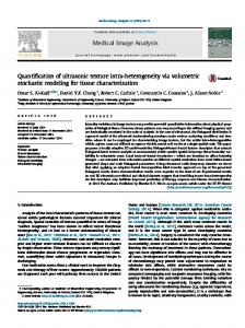
3.1 Image Analysis This section describes our method to model system orientations with images. Our model was designed to find the effects of sensor orientation on the effectiveness of triangulation, and to estimate the change in effectiveness caused by small changes in sensor orientation. These changes in orientation could
result from the user moving the sensor during normal use. Our model used drawings of detection regions from the sensor manufacturer and image analysis methods to approximate sensor performance. By using images, arbitrary shapes can be used to draw the detection area – eliminating the need for a precise mathematical model. This allows the model to be changed quickly, rather than developing new equations that describe the detection region. The theoretical detection area (found in the datasheet of the Maxbotix LV-EZ1 sensor) capable of detecting a 3.5-inch cylinder at 5V of power is shown in Figure 7(a). It shows detection to a maximum range of approximately 10.5 feet for this size object. The image was imported in Matlab as a binary image and cropped to remove empty space from all edges. Figure 7(b) shows the detection region rotated and corrected for the separation length between sensors. The correction is accomplished by padding the right edge of the image with columns filled with zeros equal to the number of columns separating the sensors. Finally, Figure 7(c) is a composite of Figure 7(b) to a copy flipped about a vertical axis. The normalized composite image displays the overlap of both sensor detection areas as white, while the area scanned by only one sensor is light grey.
In order to count the number of possible triangulation points, we fragmented the detection area image from Figure 7(a) into arcs spaced at fixed distances, each arc separated by one inch at a scale of 5 pixels per inch. The arcs must be greater than one pixel in width, and separated by a gap of more than one pixel. These conditions are used to ensure that eight-pixel connectivity can be assumed when counting connected clusters. If we assumed four-pixel connectivity, the same cluster might be counted multiple times if it is connected along a diagonal. Separating the arcs by more than one pixel ensures that there will be no diagonal connections in the composite image shown in Figure 8(b) below. The example in Figure 8 simplifies and exaggerates our method to count triangulation points. Figure 8(a) is an individual sensor image separated into arcs and Figure 8(b) is a composite image of two sensors separated an arbitrary distance. Each cluster in Figure 8(c) represents an intersection of two arcs, similar to the interference patterns of light waves. By counting the clusters (i.e., groups of white pixels surrounded by black pixels), the number of intersections can be approximated.
(a) (a)
(b)
(c)
(b)
(c)
Figure 8 (a) Sensor area represented as separate arcs. (b) Composite image of overlap for two sensors. (c) Regions from (b) approximating arc intersections.
Figure 7 (a) Model of detection area. (b) Model image rotated and adjusted for sensor separation length. (c) Composite image (normalized) of left and right side sensors.
3.2 Parametric Analysis
We calculated the average detection area width by determining the average width of the white region in Figure 7(c). To do this, we eliminated all pixels with a normalized intensity value less than one, counted the number of non-zero pixels in each row, and averaged the results over the number of rows. This process yields the average width of the white pixel area in Figure 7(c). By definition, this is the average width of the detection area within which an object can be triangulated.
When designing our system, we specified mounting one sensor on each of the user’s shoulders, thereby limiting the possible separation length between sensors. For the initial simulation, we bounded length at less than twenty inches, and rotation angle at less than eight degrees. Figure 9 and 10 show the results of the study with average width and intersection count plotted as a function of the two parameters length and angle. The average width of the sensor detection region is greatest
at small sensor separation lengths, and decreases as either the rotation angle or separation length increase. The number of intersections is not a function of rotation angle for small separation lengths, approximately ten inches or less; however, rotation angle is a factor for larger separation lengths. The simulation results suggest that changes in separation length and rotation angle increase the number of intersection points more rapidly than the same changes decrease the average detection area width. Based on the detection characteristics of the sensors, we determined a range for location and angle that allow for predictable changes if either parameter varies slightly from the design specification. We concluded that triangulation with two sensors is most effective for separation lengths greater than twelve inches with rotation angles greater than five degrees for the specific sensor used in this study (Maxbotix LV-EZ1).
Figure 9 – Variation of average detection area width over allowable separation lengths and rotation angles for two ultrasonic sensors.
3.3 Model Validation We tested two sensors spaced ten inches apart and angled towards each other five degrees from parallel in order to test the accuracy of the simulation. We placed a 3.5-inch diameter cylinder at several points near the edges of the theoretical detection range and took readings. After each reading, we moved the object towards the edge of the detection region to find the outer boundaries. Each red dot in Figure 11 is located at the furthest position at which ultrasonic measurements correctly triangulated the stationary object. We mapped these points over an image of the theoretical detection area to see how well they agree. The results obtained show that the actual detection area closely corresponds to the predicted area provided by the manufacturer’s specifications.
Figure 11 – Comparison of furthest successful test measurements to theoretical detection area; red dots represent ultrasonic measurements superimposed on the theoretical detection area.
4. Filtering Ultrasonic Sensor Readings
Figure 10 – Number of intersections, representing possible detection points, as separation distance and rotation angle vary.
We incorporated a sliding window filter with either a Kalman filter, or a Gaussian low-pass filter to stabilize the signal. The voting method used in [1] by Wijk, et. al., is essentially a threshold filter based on the number of votes received. The potential field sensor, developed in [3] by Veelaert and Bogaerts, constructs a potential field which acts as a buffer that tolerates errant readings because the system does not need to track objects moving through the field. A sliding window filter is a threshold filter, similar to a median filter [5] used in computer imaging. The purpose of the sliding window is to prevent a failure to detect small objects from corrupting the operation of the Kalman or Gaussian filter.
We added a Kalman filter [6] to improve the response characteristics of the sliding window filter. Kalman filters use a kinematic model of motion to approximate physical system behavior. When sensors detect objects in rapid motion, they are assumed to continue their path of motion instead of assuming they remain stationary during a sequence of unstable measurements. We also implemented a Gaussian low-pass filter for baseline comparison with the Kalman filter. Lowpass filters introduce lag in the response curve. The lag induced by the Gaussian filter highlights an advantage of the Kalman filter, since the Kalman filter only requires one previous data point after it is initialized to calculate the current point. We tested the filters on the detection of small objects, which the sensors frequently missed in normal operation. Figure 12 shows the response of both filters to a small object moving through the detection area. The Kalman filter provides the best combination of signal processing and lag time. However, the Gaussian filter is simpler to implement.
6. References [1] O.Wijk, P. Jensfelt and H.I Christensen. “Triangulation Based Fusion of Ultrasonic Sensor Data.” IEEE International Conference on Robotics & Automation, 1998. [2] Lei Fang, Panos J. Antsaklis, Luis Montestruque, M. Brett McMickell, Michael Lemmon, Yashan Sun, Hui Fang, Ioannis Koutroulis, Martin Haenggi, Min Xie, and Xiaojuan Xie. “Design of a Wireless Assisted Pedestrian Dead Reckoning System - The NavMote Experience.” IEEE Transactions on Instrumentation and Measurement, 2005. [3] Peter Veelaert and Wim Bogaerts. “Ultrasonic Potential Field Sensor for Obstacle Avoidance.” IEEE Transactions on Robotcis and Automation, 1999. [4] F. van der Heijden, P.P.L. Regtien. "Wearable Navigation Assistance - A Tool for the Blind." Measurement Science Review, 2005. [5] Pitas, I., Digital Image Processing Algorithms and Applications, John Wiley & Sons Inc, ISBN: 9780471377399, 2000. [6] Maybeck, P., Stochastic Models, Estimations, and Controls, Academic Press Inc., 1979. [7] H.Z. Tan, R. gray, J. J. Young, and R. Traylor, “A Haptic Back Display for Attentional and Directional cueing”, Haptics-e: The Electronic Journal of Haptics Research, Vol. 3, No. 1, pp. 20, 2003. [8] Strakowski, M.R., Kosmowski, B.B., Kowalik, R., Wierzba, P., "An ultrasonic obstacle detector based on phase beamforming principles", IEEE Sensors Journal, Vol. 6, Issue 1, pp. 179 - 186, Feb. 2006.
Figure 12 – Filter responses for a small object in the detection region.
5. Conclusions This paper analyzed the application of ultrasonic sensors to a travel aid for the blind. Triangulation and filtering techniques were used to provide distance and bearing information. A modeling technique based on image processing was used to optimize the arrangement of the sensors. Experimental testing verified the accuracy of the modeling results. Future work on this system will focus on further refinement of the triangulation techniques and integration of the distance sensors with the tactile display.
[9] Ando, B., "An Environmental Sensor Providing Home Light Classification to Blind People", Proceedings of the IEEE Instrumentation and Measurement Technology Conference, Vol. 2, pp. 1438 - 1442, May 2005. [10] Jin-Hee Lee, Eikyu Choi, Sukhyun Lim, Byeong-Seok Shin, "Wearable Computer System Reflecting Spatial Context", IEEE International Workshop on Semantic Computing and Applications 2008, pp. 153 - 159, July 2008.