USING ADAPTIVE SAMPLING TO MINIMIZE THE NUMBER OF SAMPLES NEEDED TO REPRESENT A TRANSFER FUNCTION E. K. MiIler 3225 Calle Celestial, Santa Fe, NM 87501-9613 505-820-7371,
[email protected] ABSTRACT One of the most commonly encountered problems in wave-equation applications such as arise in acoustics and electromagnetics is that of estimating transfer functions from discrete frequency samples of a first-principles, or generating model (GM) such as NEC, FERM, E-PATCH, etc. This problem has been approached in a mostly ad hoc way wherein the GM samples are spaced uniformly and closely enough such that linear i,iterpolation yields a reasonably smooth graphical representation of the continuous response. Often, additional sampling between the original ones is done subsequently to improve the result, a process that may be repeated several times until an apparently satisfactory outcome is obtained. This approach will usually result in substantial oversampling, with a concomitant increase in the associated cost, while offering no assurance that important details of the true GM transfer function have not been missed. At the same time, there is no quantitative measure of how much the linearly interpolated estimate might differ from the actual response between the sampled values. The procedure described here uses modelbased parameter estimation with rational-function, overlapping fitting models (FMs) to automatically determine where the GM needs to be sampled to reduce the mismatch between the FMs, and their estimate of the GM, below a specified value. THE BASIC IDEA As demonstrated elsewhere Wller and Burke (1991)], as a generalization of a pole series a raaonal function is a good choice for approximating an electromagnetic frequency response. The possibility of exploiting that idea to automate sampling of a first-principles, or GM subject to a specified estimation error was also considered; a more detailed description of one approach is given here. The basic idea is to use a series of rational-function FMs, Mi(ni,di), of index number i and numerator and denominator polynomial orders ni and di respectively, i = 1, . . ., N, where some of the GM samples for each Mi are shard by FMs Mi-1 and Mi+l, etc. The process begins with a small number of GM samples being computed across the bandwidth of interest and assigning a different subset of these samples to each of the initial, low-order FMs employed. A sequence of more closely spaced FM estimates is then generated from each F M . In the frequency range where two (or more) FMs overlap, the differences between these estimates are computed. The minimum match in digits, E$ and frequency where this occurs is then determined for each FM. If any of the is less than a specified estimation error, EE, a new GM sample is computed at the frequency where ME1 E min[El,EZ,. ,.,EN] occurs. This is the step that makes the process “adaptive” in that each new GM sample is
intended to yield the most additional information about the transfer function being investigated by locating it where the uncertainty in the values estimated from the FMs is greatest, as considered further below. The FMs that contain the new GM sample are then increased by one in order (alternating between increasing n and d as new GM samples are added). New 8 ' s are is detercomputed over the bandwidth spanned by the FMs thus affected and ME4, etc. until all %'s exceed EE. A mined. This process continues with final GM sample density of about 3 per resonance is achieved without initial knowledge of where these resonances are located with an EE of
w,
ESTIMATING FM ERROR OR UNCERTAINTY An adaptive process can be only as effective as the error measure used for estimating the degree to which an approximation (the FM in our case) differs from whatever process is to be approximated (the GM). This observation is a general one that applies to all manner of numerical processes having the goal of minimizing the number of samples that are needed to develop a sampled representation of some process over a specified range of independent variable@) and to thereby reduce the overall computational cost. For the present application, it is desirable to use lowerorder, overlapping FM's on subintervals of the frequency range to be covered to avoid possible ill-conditioning as well to provide a way of developing the error estimates needed to make the sampling adaptive. Since the condition number of FM M(n,d) can be of order 10"+d or larger, the FM computations need to be done in at least double precision, and maintaining n + d s 20 is advisable. The minimum match (maximum error), AMMi,j(f) I max{[IMi(f) - M,(f)l]/[lMi(f)l is then computed for each set of overlapping models as a function of frequency. Subsequent sample placement is chosen to maximize the information acquired by adding each new sample at the frequency where the minimum match, MEi, for all FMs occurs. Sampling of the GM is concluded when the specified error criterion is satisfied. Also note that, alternatively, an exact error measure results from comparing a FM result with a GM sample G(fk), using the measure AGMi,k [IG(fi) - %(fi)l]/[lG(fi) + Mk(fi)l]. However, doing this potentidly would require more GM samples with a consequent increased computer time, while providing, in addition, only a pointwise error measure in f. Thus, AMM. .(f) re1.J quires less computation and yields a global , but approximate, error measure while A G q , k requires more computation and yields a pointwise, but exact, error measure.
+ IM,(f)l]}
ADAPTIVE SAMPLING OF A SIMULATED TRANSFER FUNCTION A pole series provides a good test for an adaptive sampling strategy because many actual EM transfer functions exhibit a marked resonance structure and its properties can be specified. A 20-pole series having poles at si = 41/20 +j*i, i = 1,2, ...,20 was used as a GM with j = 4-1. The initial GM samples were placed at 0.5 intervals from s = j"3.5 to = j*ll, numbered from 1 to 16. Six FMs were employed which spanned GM sample numbers 1-6, 1-8, 5-10, 7-12, 9-16 and 11-16, respec-
583
tively. Thus, four of the six FMs (1,3,4,6) were initially of order 6, using n = 3 and d = 2, while two (2 and 5) were of order 8, using n = 3 and d = 4. The latter two FMs are arranged to include the endpoints so that there are a minimum of two overlapping FMs across the entire frequency range of interest. The estimation or, when measured in digits, EE = 2. Some results for error, EE, was set at applying the adaptive procedure outlined here are shown in Figs. 1-3. The real part of the final fitting model is shown in Fig. 1, on which are also indicated the original and additional GM samples, whose values in order of sampling, are 6.2, 7.2, 9.2, 5.3, 8.2, 9.35, 4.15, 6.25, 5.05, 1.05, 8.3, 7.05, 4.2, and 10.95. It’s also of interest to observe the behavior of the minimum-match values for each of the FMs, 4, as the process of model modification continues, a result that is shown in Fig. 2. Also shown is MEi, the minimum-match value for all six FMs, as a function of model iteration number. An I+ can remain constant for several iterations if none of the added GM samples is contained in its frequency span and its Ei is unchanged as well. Although this behavior is not guaranteed, can be see in this example to exhhit a monotonic increase. Finally, it’s significant to note, as demonstrated by Fig. 3, that the FM-FMand FM-GM mismatch errors are wellcorrelated, with the former being generally somewhat greater than the latter. This result indicates that the F M mismatch is a reliable indicator of the error between the FMs and the GM they are intended to approximate. 1.o
- v.v
1o
ORIGINALGMSAMPLES
.
.
2
‘i.i .
s - . 10
,
Fgure 1. Resutiobtainedfrom adaptive sampling of the poleseriesGM described in the text. The original 16 samples of the real part of the GM are indicated by the open circles and the additional 14 samples neededto obtain a 0.01 normalized (or twodgit) match between overlapping FMs across the 3.5 to 11 frequency range are shown as the solid circles. The final FM, obtained from averaging the individualFMs in their regionsof overlap, is shown by the solid line. The final FM-GM match is also better than 0.01
FREQUENCY
A result for the same GM as above, but with an added pole at s = -j/&O +j*7.5 using 16 initial GM samples spaced at 0.5 intervals beginning at 3.75 is shown in Fig. 6, again using an EE of 0.01. An additional 16 GM samples were required for this example, 2 more than previously because of the added pole. Although the locations of the initial GM samples are shifted relative to the poles in this case compared with the previous example, and there is an added pole in the frequency range covered by the FMs, the final performance is comparably good, indicating the robustness of the adpative-sampling approach described here.
590
Figure 2. An illustrationof how the FM parameter MEk can vary with model iteratiin number k. The Ei curve for each FM is indicated by FM(i), where the initial set of FMs is number 1 on the horizontal axis. For this particular case, ME increasesmonotonically, from less than 0 for the first several models (indicating that the normalizede r m are greater than unity) to the twodigit specified estimation error at k = 15.
1
10
0
MODEL ITERATION NUMBER
Figure 3. The average minimummatchvalues between the FMs and GM data samples for the 16th model iterationof the above example. The FM-FM minimum match is seen to be generally less than the FM-GMvalue, showing that the former is a comrvatiwe error estimate of the accuracy achieved by the FMs.
Results for the real component of the 20-pole GM used above but $ with an added pole at s = -j/nO+j*7.5 and using initial GM samples shifted by 0.25 in frequency. Shown is the averce age final FM for a 0.01 specified estimation error as obtained at the 16th additional GM sample. a
. Figure 6.
t
.
1.2'
1.0-
ADDKIONAL GM SAMPLES ORIGINAL GM SAMPLES
; -. I-
0.8
o.B.
.
LL
0 0.4-
E
2 REFERENCE
0.2-
2 ' .a0.0-r
591
.
AVERAGE FINAL REAL FM 6. GM
a
I
.
I
a