USING APPLICATION PROGRAMMING INTERFACE TO INTEGRATE REVERSE ENGINEERING METHODOLOGIES INTO SOLIDWORKS GATTAMELATA, Davide; PEZZUTI, Eugenio; VALENTINI, Pier Paolo University of Rome Tor Vergata Dept of Mechanical Engineering Via del Politecnico, 1 – 00133 – Rome – Italy Email:
[email protected]
ABSTRACT In this paper the authors present an application of Visual Basic Application Programming Interface (API) to develop numerical and procedural algorithm into CAD software. The paper focuses on Reverse Engineering embedded into Solidworks. In many RE applications there is the need to remodel the tessellated surface into an editable solid feature, to analyze it and to manipulate it. For this purpose they can be programmed numerical procedures which interact with native geometrical entities in order to improve the modelling capability using automation protocols. The presented example of API and Solidworks interaction is about the acquisition and processing of surfaces acquired by 3d laser scanner. The problem is to acquire the tessellated geometry, build up a parametric editable feature, perform topological analysis and manipulate more fragments to reconstruct an unique entity. The proposed methodology is based on the integration between native geometrical entities in Solidworks and advanced mathematics algorithms about nonlinear optimization. Both of them can be accessed and manipulated by the user using simple graphic windows. In the paper the authors describe how to implement the interaction among these entities, discussing the role of API focusing on limits and capabilities and presenting the proposed algorithms underling the critical points. Keywords: API, Reverse Engineering, Solidworks
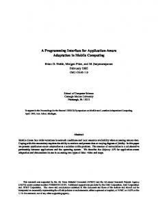
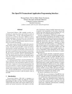
1. Introduction to Solidworks & API Solidworks is a widely used commercial software about engineering modelling and computer aided design. It is based on parametric definition of component and feature and it can be used in a very intuitive way. Although recent releases include many packages, Reverse Engineering applications [14] are only limited to the module FeatureWorks about the automatic feature recognition of external parts. There is no way to process a point cloud o manipulate meshed file (such as stereolithography, .stl) which are treated only as graphical primitives. Other engineering modellers (such as Catia) have dedicated module to RE application, but the purchase of their license may be very expensive. Specific RE software (such as Rapidform) does not allow the building of parametric feature-based models. In many cases there is also the need to implement specific algorithm to perform dedicated an accurate computation which can not be found in any commercial software. These are the main motivations to use Application Programming Interface within a commercial software. This allows to use the predefined native geometrical entities and operations together with an home made computational algorithm. Recent Solidworks releases have improved the methods supported by native object and they have been interlaced with a very powerful Mathematical Utility. This feature allows to easily perform basic and advanced point, vector and matrix operations. Using API into Solidworks we can manipulate three kinds of objects: those coming from Solidworks (model native entities), those coming from math utility database (math entities) and user defined entities (Figure 1). The native geometrical objects concern the sketch entities (point, line, circle, spline, etc.) and their constraints, the features (extrusion, revolution, loft, etc.), the assembly management (mating, inserting, moving, etc.). The math native objects concern points, vectors and transformations for manipulate entities (projecting from model space to sketch space and vice versa, performing basic operation on vectors, etc.).
Figure 1: Solidworks API entity scheme Using the software without API the user can only access to single model entity and the direct access to internal database is not permitted [8]. Using API the database of entity can be directly accessed saving time to execute command and model entities can be interlaced with math and user defined ones. Let us consider to import a list of points. If the number of these points is huge, importing by hand is impossible, so it can be generated a macro command to repeat the operation of importing one point for all the points to be processed. Although this operation is possible it is not the best way. The smartest way to import points is to access directly to internal Solidworks database, this can be only done with API programming techniques. In order to have an idea of time difference in importing points using macro command, we have tested the operation of reading 1000 points from an ASCII file and importing into model using a desktop pc. If we use standard access to database the entire process takes 1 min and 35 s, if we perform a direct database access it takes less than 1 s (more than 90 times faster!). Optimizing processing time is very important especially for RE application where the entity (points, mesh, etc.) to manage are so many. For direct database access the native method is SetAddToDB(True) which has to be applied to the current document (part or assembly). The programmer can use also the method SetDisplayWhenAdded (True) to avoid to display entities details when they have been created. Both of them represent a smart way to import numerous entities.
When a sketch point has been created its properties are read only, thus they cannot be modified. In order to perform point operations the programmer can create a point/vector alias in the math space using the methods CreatePoint(vector)/CreateVector(vector) which has to be applied to the current document MathUtility. The programmer can get also the transformation matrix to perform both point and vector operation. In Solidworks it have to be expressed as 4x4 matrix [TRANS]:
Where
[ R]
⎡[ R ] [t ] ⎤ [TRANS ] = ⎢ 3 x3 3 x1 ⎥ ⎢⎣ [ n ]1x 3 [ s ]1x1 ⎥⎦
is the matrix describing rotation about x, y, and z axis,
(1)
{t}
is the vector describing
translation along x, y and z axes, {s} is the scaling vector and {n} is an unused vector.
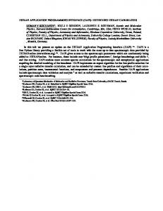
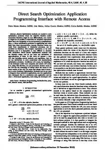
Figure 2: Steps to rebuild a featured surface: 1. importing mesh, 2. computing revolution axis (only for axial-symmetric shape), 3. sectioning with splines, 4. surfacing with loft or fill.
2. Surface reconstruction algorithm details The first developed routine is about a common Reverse Engineering problem [5]: the reconstruction of a 3d fetured surface starting from a point cloud. We can split the problem into four activities. First, we have to import a stereolithografy mesh (.stl) coming from the automatic acquisition system (taster, scanner, etc.). In order to perform this task in a smart way we have used the direct database access as described in the introduction. Then we have to process the mesh. Two are the principal operations which have been implemented. The first is the search for hypothetic revolution axis. If the mesh coming from a shape which have a revolution axis the knowledge of this axis can be very useful for further manipulation (see section 3). In order to assess the axis of a discretized surface
we can use the Halir method [6-7]. This methodology has been successfully applied by the authors in a previous work [8]. In this paper we present a modified algorithm which seems to be more stable and more accurate. This method is suggested especially for .stl mesh because this format includes information about the normal vector of each patch. The idea starts from the consideration that the normal vectors to a revolution surface pass through the axis of revolution. This axis can be found minimizing the sum of residuals of distance between surface points normal vectors and a parametric expression of the axis. Assuming the G revolution axis a to be:
G G G a = O + t ⋅ no
G G G and defining for generic point X i with normal vector ni the normal axis N as G G G N i = X i + s ⋅ ni
(2)
(3)
we can compute the distance between normal vectors and revolution axis as:
G G G G X i − O ⋅ ( ni × n0 ) G G di N i , a = G G ni × n0 G The six unknown parameters of axis a can be found by solving: G G min ∑ di 2 N i , a
(
(
)
(
)
)
(4)
(5)
i
According to the authors’ experience the implementation of the optimization routine for (5) G leads to instability and inaccuracy due to the absence of an normalization of vector n0 . This behaviour can be explained notice that in order to solve the (5), even sophisticated numerical procedures find solutions near the null vector; this causes the inaccurate determination of the direction cosines of axis G a . The normalization condition can be added to the problem leading to a constrained optimization problem which requires an accurate nonlinear programming tool. Since the normal vector coming G from .stl files are already normalized, and including the normalization condition for vector n0 the distance in (4) can be simplified as:
G G G G G G di N i , a = X i − O ⋅ ( ni × n0 )
(
) (
)
(6)
And the optimization can be rewritten as
G ⎧min ∑ di 2 N i , aG ⎪ i ⎨ G G ⎪⎩ n0 ⋅ n0 = 1
(
)
(7)
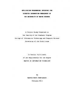
In order to improve the accuracy of solution for irregular meshes with patches of different area, we can weight the distance with the same area value. For detailed or regular meshes this remedy gives no benefit. The third implemented procedure is the slicing of the imported mesh. For sake of brevity we discuss only the outline of the proposed algorithm which is reported in Figure 3. The idea is to create a set of parallel planes and to intersect the meshes. If an imported point is sufficiently near to the cutting plane, it is projected onto it. For projecting the point we can use the math transformations as discussed in the introduction which allow to use native procedures. The method that seems suitable is GetClosestDistance, which returns the distance between two entities and the projected point coordinates at the same time. Then, for each cutting plane a spline is created interpolating all the projected points. Particular attention has been paid to the orienting of points for improve coherency of spline (Figure 4). Having a set of n points there are n! splines which can interpolate them. Only one of these curves matches the actual profile. When you manage a lot of points some error may occur. These pitfalls may be avoided using an accurate ordering procedure.
Figure 3. The proposed algorithm for point cloud cutting According to author experience a simple clockwise (or counter clockwise) ordering of points does not allow to avoid ordering defects. For this reason the authors propose the following algorithm. Starting from a first reference point the spline is created searching the nearest point to the previous one, paying attention that the orientation of the tangent vector of the spline does not has quick variation (more than 90° in two adjacent points). Ambiguous points are filtered out. This algorithm intrinsically filters out boundary spikes, outliers, etc.
Figure 4: Ordering defects in creating cutting section splines: correct spline, self reversing spline and a self intersecting spline. The forth procedure which has been implemented is the remodelling of the featured surface starting from section splines. There are two methods to build the surface. The first is based on the lofting through the sections, the second is based on the filling surface among the contour surfaces respecting the section splines as constraint of interpolation. The authors experience some difference between the two methodologies. The first one requires lower computational effort and it is suitable for a huge number of cutting section. If one has to manage with a small number of section, it can be made a refinement creating some fictitious intermediate splines in order to increase accuracy. The second methods has the advantage to constraint the surface not only with the cutting sections but also at the boundaries. This is useful to create geometrical edges for further investigations (see next section). On the other hand, a large number of cutting section may generate instability of interpolation (Figure 5).
Figure 5: Difference in interpolating surface: lofting on the left and filling on the right. Notice the difference in accuracy and the presence of unwanted ripples on the filled surface.
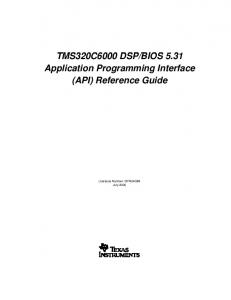
3. Manipulating entities If the purpose of the acquired geometries is to reconstruct a single shape starting from its fragments, some methodologies for manipulating and matching them have to be embodied as well. In this case the API can be useful to automate the computational algorithm for collecting geometrical data and matching the right entities. All these tasks can be performed into an assembly document where two or more fragments have been imported. The target is to compute the right movement to bring one fragment very close to another in a consistent position to perform a stitching of surfaces. A numerical procedure, integrated into CAD, can solve an optimization problem (minimizing the gap between two lateral edges) avoiding manual attempt for positioning the components and measuring reconstruction errors. An example concerning shapes with a common revolute axis (i.e. pots, amphorae, etc.) is herein discussed. If the fragments have been processed using algorithm presented in the previous section, for each of them we know the bounding edges and the revolution axis. The complete matching procedure can be split into six main steps (Figure 6): 1. Importing the fragments and matching the axes; 2. Collecting edges data; 3. Searching for consistent starting point; 4. Finding drag parameters; 5. Checking correspondent points distance; 6. Final matching. The first fragment which is imported into the assembly document can be considered as a reference fragment and it is assumed to be fixed. Then, the second fragment can be imported and its revolution axis has to be constrained to be coincident to the revolution axis of the first one (step 1). At this step, the unknown 2nd component positioning variables for matching lateral edges are the displacement along the common axis and the rotation angle about it (2 d.o.f.). In order to solve the problem, we have to analyse and compare the lateral boundary edges. For this purpose the geometrical data of these entities have to be acquired (step 2). This task can be performed using the method GetBCurveParams which, acting on a spline, returns a unique vector listing the number of knots, the number of control points, the knots values and the control points coordinates (x, y, z). In order to get spline points it can be used the method GetSplinePts, which computes the interpolation points starting from the control ones and the knots values. It is important to underline that the described method returns coordinate values in each component local reference frame. In order to transform these coordinates in the global (assembly) reference frame, we have to build an appropriate transformation matrix. Using API with Solidworks this matrix can be computed with the method Transform2 which acts on a Component2 object and returns a matrix like that in (1). Coordinate vectors can be transformed defining mathematical points dual entities as described in the first section (with MathUtility::CreatePoint) and then applying the transformation (with MultiplyTransform acting on mathematical point). Once the boundary edges are described in terms of global reference frame, the matching algorithm can be applied (step 4).
Let us now focus on this numerical procedure details (Figure 7). Since the boundary edges have been generated with the algorithm discussed in the previous section, using small distance between sectioning planes, they have been defined with a lot of interpolating points which are uniformly spaced. Assuming that the first edge has N1 points and the second edge has N 2 points (with N 2 ≤ N1 ), we can define the number of possible placing configurations as Nt = N1 − N 2 + 1 . Each configuration represents the mating between edges starting from a different height (different point). In the first one, the point P11 on the first edge contacts the point P12 on the second edge; in the second one, the point P21 on the first edge contacts the point P12 on the second edge; in the i-th configuration, the point Pi1 on the first edge contacts the point P12 on the second edge.
Step 1: Importing the fragments and matching the axes
Step 2: Collecting edges data (N1=5, N2=3)
Step 3: Searching for consistent starting point
Step 4: Finding drag parameters
Step 5: Checking correspondent points distance
Step 6: Final matching
Figure 6: Steps for fragments registering For each configuration we can compute the distance between the starting points and the common axis. If the difference (Diff, in Figure 7) of the two distances is less than a tolerance value, then the configuration can be considered as admissible. In this case we can move the second frame in order to bring the two starting points at the same position (step 4). This movement can be performed using the method DragOperator::Drag which acts on the second fragment two times. The fist time is for rotating the components and it requires the definition of a transformation matrix which can be done using MathUtility::CreateTransformRotateAxis. The second time the method translates the component along the axis and it requires the definition of a transformation (translation) matrix using MathUtility::CreateTransform. The check on only starting points is not sufficient for a global matching. It only means that locally the distance from the common axis is the same. This condition has to be verified globally on the edge. Actually, the fragments can have only a part of the edge in contact, and so the global matching condition can be replaced with a sufficient length ( ∆z ) matching condition (depending on
fragments leading dimension) among N ∆z points. For this purpose we can define the gap function PF of the i-th possible configuration as:
PF ( i ) = G
N ∆z
∑ k =1
G G Pk1+i − Pk2
2
(8)
G
where Pk1+i is the vector of the (k+i)-th point on the first fragment edge and Pk2 is the vector of the kth point on the second fragment edge. If the value of this function is less than a tolerance, the congruence between the two edge for the i-th configuration can be considered acceptable, and the iteration can be stopped. On the contrary, the movement is a fake and iteration has to continue.
Figure 7: Matching algorithm The proposed algorithm has been tested on several fragments and some numerical remarks can be underlined. The first comment is about the tolerance to be chosen for matching. Point clouds coming from acquisition may have some imperfections on the extremities due to measuring errors or physical defects on surface. Moreover the computation of revolution axis may be quite imprecise. For both these reasons, the spline defining boundary edges may be affected by errors. Thus, the tolerance value has to be not so small. Authors experienced that best value for 10 cm x 10 cm fragments are within the range 1÷2 mm. In case of small fragments or fragments with small curvature variation, congruent configurations may be more than one. In this case it can be useful to perform the iteration for all of them instead of stopping to the first congruent position. The DragOperator is able to check collisions avoiding interference in component positioning. This property can be useful to avoid configuration which seems congruent but leads to unphysical results (self intersecting surfaces)
4. Conclusions Tests on the proposed methodology integrating API and Solidworks for Reverse Engineering applications, confirmed the power of integrating numerical algorithm into CAD. The direct access to
geometrical entities and the possibility to create alias mathematical entities or user defined objects revealed to be a valid instrument to improve the reliability of manual procedures and to reduce the time for computation. Two interlaced problems have been faced. The first is about the building of a 3d featured model from an acquired point cloud. In this case the use of direct access to database has given great advantages. Moreover the procedures for revolution axis determination and automatic sectioning discussed in detail has been tested an revealed to be robust. The second faced problem is about the manipulation of the modelled fragments in order to search for a possible matching to reconstruct a unique shape. In this case an other algorithm, based on the minimization of spline points, has been presented. Although this research activity is quite recent, the presented examples give an idea of the great capabilities of programming into a CAD environment. This synergy can link the advantage of a globally used software about reliability, graphical capabilities and pre-implemented procedures, with own made numerical procedure to solve specific problems, without the difficulties to build up a specific graphical engine.
References [1] Wills, L.M., Newcomb, P., Reverse Engineering, Springer, 1996 [2] Hoschek, J., Dankwort, W., ed., Reverse engineering, Stuttgart Teubner, 1996 [3] Várady, T., Martin, R.R., Cox, J., Reverse engineering of geometric models – an introduction, ComputerAided Design, vol. 29(4), pp. 225-268, 1997 [4] Werner, A., Skalski, K., Piszczatowski, S., Święszkowski, W., Lechniak, Z., Reverse Engineering of freeform surfaces, Journal of Material Processing Technology, vol. 76, pp. 128-132, 1998 [5] Chivate, P.N., Jablokow, A.G., Solid-model generation from measured point data, Computer-Aided Design, vol. 27(12), pp. 905-914, 1995 [6] Halir R., An Automatic Estimation of the Axis of Rotation of Fragments of archaeological pottery: a multistep approach, Proceedings of the 7-th WSCG International Conferences in Central Europe, 1999 [7] Cao Y., Mumford D, Geometric Structure Estimation of Axially Symmetric Pots from Small Fragments, Proceedings of the SHAPE Lab. @ SPPRA'02 Signal Processing, Pattern Recognition and Applications IASTED International Conference, 2002 [8] Pezzuti, E., Piscopo, G., Ubertini, A., Valentini, P.P., Milana, M., Di Leginio, R., Una metodologia per l’analisi e l’archiviazione di reperti archeologici basata sul rilievo mediante scanner laser tridimensionali a non contatto, Archiviazione e Restauro di Reperti Archeologici Mediante Tecniche CAD-RP (in italian), Napoli, 2004 [9] Bidalach, I., Portal, R., Dias, J.P., Integration of CAD and Multibody Systems, Proceedings of ECCOMAS Multibody Dynamics 2005, Madrid, 21-24 June 2005.