International Journal of Applied Engineering Research ISSN 0973-4562 Volume 12, Number 5 (2017) pp. 671-680 © Research India Publications. http://www.ripublication.com
Using of Fuzzy PID Controller to Improve Vehicle Stability for Planar Model and Full Vehicle Models Abdusslam Ali Ahmed1 Institute of Natural Sciences, Okan university/Istanbul, Turkey. E-mail:
[email protected] 1
ORCID: 0000-0002-9221-2902
Başar Özkan2 Mechanical Engineering Department, Okan university/Istanbul, Turkey. E-mail:
[email protected]
Abstract Stability control system plays an important role in vehicle dynamics in order to improve the vehicle handling and stability performances. In this paper, vehicle stability control system is studied by using of two vehicle models which are a planar vehicle model and full vehicle model, design of a complete vehicle dynamic control system is required to achieve high performance of vehicle stability and handling, this control system structure includes three parts which are a reference model (2 DOF vehicle model) used for yaw stability control analysis and controller design, actual vehicle model, and the controller. In this work a fuzzy PID controller was used and designed to improve the stability of the vehicle. Many simulation results show the structures of control systems for vehicle models used in this work were successful and can improve the handling and stability of the vehicle.
(AFS), and active four-wheel steering control (4WS); 3) traction/braking, e.g. anti-lock brake system (ABS), electronic stability program (ESP), and traction control (TRC).[1]. Based on our survey of research trends in this topic, many researchers have worked about vehicle dynamics control, stability, handling, and passengers comfort. All works give very practical results for specific estimation parameters like lateral acceleration, yaw rate and sideslip angle but most of researchers used just vehicle planar models in their studies with many control methods that means they didn’t take into consideration heave, pitch, and roll motions of sprung mass. Some studies[2,3,4] discuss the stability control for electric vehicle in general and used planar vehicle model and sliding mode control method theory in their studies, while another works also used planar model to study handling and stability of vehicles but with different control strategies such as using of H∞ control theory [5], designing of controller dynamically allocates the drive torque in terms of the vertical load and slip rate of the four wheels[6],robust control method [7] to preserve vehicle stability and improve vehicle handling performance, and Fuzzy PID Method[8] to improve yaw stability control for in-Wheel-Motored electric vehicle.
Keywords: vehicle model, Fuzzy PID controller, vehicle stability, yaw rate, Planar vehicle model, Full vehicle model. INTRODUCTION Thanks to the development of electric motors and batteries, the performance of EV is greatly improved in the past few years. The most distinct advantage of an EV is the quick and precise torque response of the electric motors. A further merit of a 4 in-wheel-motor drived electric vehicle (4WD EV) is that, the driving/braking torque of each wheel is independently adjustable due to small but powerful motors, which can be housed in vehicle wheel assemblies. Besides, important information including wheel angular velocity and torque can be achieved much easier by measuring the electric current passing through the motor. Based on these remarkable advantages, a couple of advanced motion controllers are developed, in order to improve the handling and stability of a 4WD EV [17].
Other researches[9,10,11,12,13,14,15] in vehicle dynamic field discussed the handling and stability in cars with many control techniques and they took into account the full model of vehicle which includes the suspension system and rotational motions: yaw motion, pitch motion, and roll motion. The main different between this work and the other is using of Fuzzy PID controller with both of planar vehicle model and full vehicle model to improve stability and handling. The proposed control architecture in this paper similar control architecture was used in [16] for the simulation of vehicle stability control system in addition of rolling, pitching, and bouncing of the sprung mass in the case of full vehicle model.
Modern motor vehicles are increasingly using active chassis control systems to replace traditional mechanical systems in order to improve vehicle handling, stability, and comfort. These chassis control systems can be classified into the three categories, according to their motion control of vehicle dynamics in the three directions, i.e. vertical, lateral, and longitudinal directions: 1) suspension, e.g. active suspension system (ASS) and active body control (ABC); 2) steering, e.g. electric power steering system (EPS) and active front steering
VEHICLE MODELS In this paper, three types of vehicle dynamic model are established: a non-linear vehicle planar dynamic model, full vehicle model developed for simulating the vehicle dynamics, and a linear 2-DOF reference model used for designing
671
International Journal of Applied Engineering Research ISSN 0973-4562 Volume 12, Number 5 (2017) pp. 671-680 © Research India Publications. http://www.ripublication.com controllers and calculating the desired responses( desired vehicle yaw rate and desired sideslip angle) to driver’s steering input. This work includes comparing of vehicle stability performance in the case of using of planar vehicle dynamic model and the other case which is full active vehicle model.
Full Vehicle Model A vehicle dynamic model is established and the three typical vehicle rotational motions, including yaw rate motion, the pitch motion, and the roll motion, are considered. They are illustrated in Figure. 2(a), Figure. 2(b), and Figure. 2(c), respectively. The equations of motion can be derived as: For yaw motion of sprung mass shown in Figure. 1(a) w z I z I xz a( FxfR sin( ) FyfR cos( ) FxfL sin( ) FyfL cos( )) b( FyrL FyrR )
Planar Vehicle Model This vehicle model is a four-wheel vehicle, only considering the planar motion: longitudinal, lateral, and yaw. And the vehicle is modeled as a rigid body with three-degree-of-freedom. The bob, pitch and roll motions are ignored. Figure 1 shows the vehicle diagram with planar motion.
(4) Where wz is the vehicle yaw rate, Iz is yaw moment of inertia of sprung mass ,a and b is horizontal distance between the C.G. of the vehicle and the front, rear axle, and ϕ is the roll angle of sprung mass. The equations of motion in the longitudinal direction and the lateral direction can be written as: m(v x v y wz ) ms hw z [ FxfR cos( ) FyfR sin( ) FxfL cos( )
FyfL sin( ) FxrL FxrR ] f r mg (5) Where m is the mass of the vehicle , vy is the vehicle speed in the lateral direction, vx is the vehicle speed in the longitudinal direction is the , h is the vertical distance between the C.G. of sprung mass and the roll center , and fr is the rolling resistance coefficient. m(v y v x wz ) ms h [( FxfR sin( ) FyfR cos( ) FxfL sin( ) FyfL cos( ) FyrL FyrR ]
Figure 1: Planar Vehicle Model.
(6) For pitch motion of the sprung mass:
I y b( Fz 3 Fz 4 ) a( Fz1 Fz 2 )
The differential equation of vehicle motion is shown as follows: For yaw movement: Iw z [a( FxfR FxfL ) sin( ) a( FyfR FyfL ) cos( ) b( FyrL FyrR )
(7)
d d d ( FxfR FxfL ) cos( ) ( FxrR FxrL ) ( FyfL FyfR ) sin( )] 2 2 2
(1) For longitudinal movement: v x v y wz
1 [( FxfR FxfL ) cos( ) ( FyfR FyfL ) sin( ) FxrL FxrR ] m
(2) For lateral movement: 1 v y vx wz [( FyfL FyfR ) cos( ) ( FxfL FxfR ) sin( ) FyrL FyrR ] m (3) Whrer
Fx fR , FxfL , FxrR , FxrL , FyfR , FyfL , FyrR ,
FyrL are force components for front right, front left, rear right and rear left tire along x, y coordinates respectively; a ,b the distance of the center of gravity of the vehicle to front and rear axle; d distance between leaf and right wheels; vx, vy longitudinal and lateral velocity , wz yaw rate, δ is the front wheel steering angle, m is the total vehicle mass, I is the moment of inertia of the vehicle about its yaw. Figure 2: Three typical vehicle rotational motions: (a) yaw motion; (b) pitch motion; (c) roll motion.
672
International Journal of Applied Engineering Research ISSN 0973-4562 Volume 12, Number 5 (2017) pp. 671-680 © Research India Publications. http://www.ripublication.com
Fz1 , Fz 2 , Fz 3 , Fz 4 in equation (7) are the total force of the suspension acting on the front and rear sprung masses, Iy is the pitch moment of inertia of sprung mass , and θ is the pitch angle of sprung mass.
(19)
Z s 3 Z s b d
(20)
Z s 4 Z s b d
(21)
Vehicle Reference Model In vehicle dynamic studies, the reference vehicle model as shown in Figure 3 is commonly used for yaw stability control analysis and controller design. This model is linearized from the nonlinear vehicle model based on the some assumptions: Tires forces operate in the linear region, the vehicle moves on plane surface/flat road (planar motion), and Left and right wheels at the front and rear axle are lumped in single wheel at the center line of the vehicle.
And for roll motion od sprung mass: z ms gh d ( Fz 2 Fz 3 Fz1 Fz 4 ) I x ms (v y vx wz )h I xz w (8) Where Ix is the roll moment of inertia of sprung mass and Ixz is the product of inertia of sprung mass about the roll and yaw axes. We also have the equations for the vertical motions of sprung mass and unsprung mass.
ms Zs Fz1 Fz 2 Fz 3 Fz 4
Z s 2 Z s a d
(9)
Z s is the vertical displacement of sprung mass. mu1 Zu1 k t1 (Z g1 Z u1 ) Fz1 m Z k (Z Z ) F
Where
u2
u2
t2
g2
u2
z2
mu 3 Zu 3 k t 3 (Z g 3 Z u 3 ) Fz 3 mu 4 Zu 4 k t 4 (Z g 4 Z u 4 ) Fz 4
(10) (11) (12) (13) Figure 3: Vehicle refernce model(bicycle model).
Where mui is the mass of the unsprung mass at wheel i., Zui is the vertical displacement of unsprung mass, kti is the stiffness of tire at wheel i, and Zgi is the road excitation. The total force of the suspension acting on the front and rear sprung masses can be calculated as: k af ( Z Z u1 ) Fz1 k s1 ( Z u1 Z s1 ) c1 ( Z u1 Z s1 ) u2 f1 2d 2d (14) Fz 2 k s 2 ( Z u 2 Z s 2 ) c2 ( Z u 2 Z s 2 )
k af ( Z Z u1 ) u2 f2 2d 2d (15)
k Fz 3 k s 3 ( Z u 3 Z s 3 ) c3 ( Z u 3 Z s 3 ) ar 2d
(Z u 3 Z u 4 ) f3 2d (16)
k ar 2d
(Z u3 Z u 4 ) f4 2d (17)
Fz 4 k s 4 ( Z u 4 Z s 4 ) c4 ( Z u 4 Z s 4 )
The driver tries to control the vehicle’s stability during normal and moderate cornering from the steer ability point of view. Therefore, the reference model reflects the desired relationship between the driver performance and the vehicle stability factors. Hence, the model is designed to generate the desired values of the yaw rate and the sideslip angle at each instance, according to the driver’s steering wheel angle input and the vehicle velocity, while considering a constant forward velocity. The desired sideslip angle of the vehicle is tried to be maintained as closest as possible to zero, since a vehicle slipping to the sides is not a desired behavior. d 0 On the other hand, while cornering, the yaw rate value cannot be assumed as zero. Instead, it has to have a value that depends on the front wheel inclination angle, the forward velocity and the vehicle dimensions, and could be calculated as follows [37]: vx wzd ( L) 1 kusvx2 (22)
Where ksi is the stiffness of the suspension at wheel i , ci is the damping coefficient of the suspension at wheel i, kaf is the stiffness of the anti-roll bars for the front suspension, kar is the stiffness of the anti-roll bars for the rear suspension , and fi is the control force of front and rear active suspension controller. When the pitch angle of sprung mass θ and the roll angle of sprung mass ϕ are small, the following approximation can be reached. (18) Z s1 Z s a d
kus m( Lr Car L f Caf ) / LCaf Car
(23)
Where wzd and βd are the desired yaw rate and desired sideslip angle, kus is the understeer parameter, and Caf , Car are longitudinal and lateral stiffness of front and rear tire. The simulation result for the vehicle reference model which represents the desired yaw rate is shown in Figure 4.
673
International Journal of Applied Engineering Research ISSN 0973-4562 Volume 12, Number 5 (2017) pp. 671-680 © Research India Publications. http://www.ripublication.com
Fy C2
tan f ( ) 1 x
(29)
Where C1 and C2 are the longitudinal and cornering stiffness of the tire,
x is the longitudinal slip ratio of
the tire and defined in equation 30 and equation 31,and i is the tire slip angle at each tire.
R w i vx v x 1 x Rw i
x 1
T2 Fx 2 .Rw
T3 Fx3 .Rw I w 3 T4 Fx 4 .Rw I w 4
Figure 5:
(24)
(26)
(32)
fL
v a.w z tan 1 y d v .w x z 2
(33)
v b.w y z rL tan v d .w x z 2
(34)
v b.w z rL tan 1 y v d .w x z 2
(35)
1
(27)
The variable and the function f ( ) are given by Fz (1 x ) (36) 2 {(C1 x ) 2 (C2 tan( )) 2 }
Wheel schematic diagram.
x f ( ) 1 x
fR
v a.w z tan 1 y v d .w x z 2
(25)
And
TIRE MODEL At extreme driving condition, the tire may run at non-linear religion. This paper uses Dugoff’s tire model which provides for calculation of forces under combined lateral and longitudinal tire force generation.. The longitudinal and lateral force of tire were expressed as [11]:
Fx C1
(31)
vehicle geometry and wheel vehicle velocity vectors. If the velocities at wheel ground contact points are known the tire slip angles can be easily derived geometrically and are given by:
MODEL OF WHEEL DYNAMIC A schematic of a modeled wheel is shown in Figure 5. The wheel has a moment of inertia Iw and an effective radius Rw. Torque T can be applied to the wheel and longitudinal tire force Fx is generated at the bottom of the wheel. The wheel rotates with angular velocity ω and moves with a longitudinal velocity vx. A summation of the moments about the axis of rotation of the wheel generates the dynamical equation shown in following equation:
I w 2
in the case of acceleration
(30)
The individual tire slip angles i are calculated using
Figure 4: The desired yaw rate of the vehicle reference model.
T1 Fx1 .Rw I w1
in the case of deceleration
f ( ) ( 2 ) f ( ) 1
if 1
if 1
Where is the tire-road friction coefficient and vertical tire force for each wheel.
(28)
(37)
Fz is the
FUZZY PID CONTROLLER Fuzzy PID controller is composed of adjustable PID controller and fuzzy controller. The core is fuzzy controller. It contains
674
International Journal of Applied Engineering Research ISSN 0973-4562 Volume 12, Number 5 (2017) pp. 671-680 © Research India Publications. http://www.ripublication.com fuzzification, repository, fuzzy inference, defuzzification, and input/output quantification and so on. Fuzzy logic is a rule which can map a space-input to another space-output. In engineering application, fuzzy logic has the following characters: 1) Fuzzy logic is flexible; 2) Fuzzy logic is based on natural language, and the requirement for intensive reading of data is not very high; 3) Fuzzy logic can take full advantage of expert information; 4) Fuzzy logic is easy to combine with traditional control technique. Fuzzy PID controller takes E (the error between feedback value and desired yaw rate value of controlled station as input. Using fuzzy reasoning method it adjusts the PID parameters (Kp, Ki, Kd). Change the PID parameters on line by using the fuzzy rules; these functions form the self-setting fuzzy PID controller. Its control system architecture is shown in Figure 6.
CONTROL STRATEGY In this paper the Fuzzy PID Controller is designed to improve the vehicle yaw stability in the case of vehicle planar model and the full vehicle model. The fuzzy PID controller can be decomposed into the equivalent proportional control, integral control and the derivative control components. we design a control system which includes three parts: the reference vehicle model(Bicycle model), full vehicle model( Actual vehicle), and the fuzzy PID controller. The structure of the two vehicle models with controller are given in Figure 7 and Figure 8. Depending on 𝛿 which can be gained by the driver action and vx, the expected vehicle’s yaw rate wzd can be calculated through the reference model. The PID controller is applied widely, because it possesses the virtues such as the simple structure , better adaptability and faster response time. Regulating the parameters of the PID is the fussy task by manual work, while regulating parameter by fuzzy controller is very convenient. The sideslip angle 𝛽 is compared with desired sideslip 𝛽𝑑 and the yaw rate wz is compared with desired yaw rate wzd, and then the yaw rate is calculated. The fuzzy control is implemented as follow: the input variable, i.e., vehicle yaw rate error, is fuzzificated firstly, and then the output variables, the direct yaw moment Mz. The fuzzification is the process of transforming fact variables to corresponding fuzzy variables according to selected member functions.
Figure 6: The structure of fuzzy PID controller.
Figure 7: The structure of vehicle model with controller for planar model.
Figure 8: The structure of vehicle model with controller for full vehicle model.
675
International Journal of Applied Engineering Research ISSN 0973-4562 Volume 12, Number 5 (2017) pp. 671-680 © Research India Publications. http://www.ripublication.com SIMULATION RESULTS AND DISCUSSION In this paper, the simulation models are a planar vehicle model which includes longitudinal, lateral, and yaw motions only and a full vehicle model that includes active suspension dynamics, roll, yaw and pitch motion. Using the vehicle speed, yaw rate, longitudinal and lateral accelerations of the vehicle at c.g. As the measurement vectors, the steering angle as input signal. The control system is analyzed using Matlab/Simulink. We assume that the vehicle travels at a constant speed vx = 20m/s, and is subject to a steering input from steering wheel. The steering input is set as a step signal which sown in the figure 9. The values of the vehicle physical parameters used in the simulations are listed in Table 1. Table 1. vehicle physical parameters. Parameter
Unit
Value Parameter
Unit
Value
ms
Kg
810
c1
KN.s/m
1570
m
Kg
1030
c2
KN.s/m
1570
a
m
0.968
c3
KN.s/m
1760
b
m
1.392
c4
KN.s/m
1760
d
m
0.64
ks1
KN/m
20.6
Rw
m
0.303
ks2
KN/m
20.6
Iw
Kg.m2
4.07
ks3
KN/m
15.2
μ
---
0.4
ks4
KN/m
15.2
C1
KN/rad 52.526
kaf
(N.m/ rad)
6695
C2
KN/rad 29000
kar
(N.m/ rad)
6695
Caf
KN/rad 95.117
Ix
Kg.m2
300
Car
KN/rad 97.556
Iy
Kg.m2
1058.4
g
m/s2
9.81
Iz
Kg.m2
1087.8
mu1
Kg
26.5
v0
m/s
20
mu2
Kg
26.5
fr
---
0.015
mu3
Kg
24.4
h
m
0.505
mu4
Kg
24.4
Figure 9: The angle of front steering wheel on step maneuver.
In this paper, the mathematical model for vehicle dynamic model has been presented above for planar vehicle model and full vehicle model. Figure 10-Figure 14 present the selected results of the planar vehicle model with and without control. Figure 10 and Figure 11 present the longitudinal velocity and lateral acceleration of the vehicle while, Figure 12 shows Comparison between the vehicle yaw rate with and without control and (Figure 13) presents the Comparison between Sideslip angle with and without control. Fuzzy rule viewer shown in Figure 14 gives the effect of control signal for change in rules. Finally it's obvious that using of Fuzzy PID controller improved the vehicle stability performance.
Figure 10: Comparison between longitudinal velocity with and without control.
676
International Journal of Applied Engineering Research ISSN 0973-4562 Volume 12, Number 5 (2017) pp. 671-680 © Research India Publications. http://www.ripublication.com
Figure 11: Comparison between Lateral acceleration with and without control.
Figure 14: Rule viewer of fuzzy PID controller in the case of planar vehicle model The simulation results of the full vehicle model are shown in Figure 15-Figure 18, these simulation results illustrate comparison of the full vehicle model with and without fuzzy PID controller. Also, in this model the vehicle stability performance with fuzzy PID controller is improved. Fuzzy rule viewer shown in Figure 19 gives the effect of control signal for change in rules.
Figure 12: Comparison between yaw rate with and without control.
Figure 15: Comparison between longitudinal velocity with and without control.
Figure 13: Comparison between Sideslip angle with and without control.
677
International Journal of Applied Engineering Research ISSN 0973-4562 Volume 12, Number 5 (2017) pp. 671-680 © Research India Publications. http://www.ripublication.com
Figure 16: Comparison between Lateral acceleration with and without control.
Figure 19: Rule viewer of fuzzy PID controller in the case of planar vehicle model
CONCLUSION Aiming at improving vehicle stability,the simulink model of the vehicle is constructed with Fuzzy PID controller to ensure and improve the vehicle stability in this paper. The results and plots show a significant difference between the vehicle performance in the case of without control and the vehicle stability and performance in the case of using Fuzzy PID controller. Also, it is found that, using Fuzzy PID controller with both of planar and full vehicle models was successful in improve the vehicle performance. The lateral acceleration, yaw rate , and sideslip angle improved significantly. Therefore vehicle stability control system using fuzzy PID controller can enhance the performance and stability of vehicle. Figure 17: Comparison between yaw rate with and without control.
ACKNOWLEDGEMENT I express my deep thanks to the Asst.Prof.Başar Özkan for his support and guidance in this work. REFERENCES [1] R. Rajamani, Vehicle dynamics and control: Springer Science & Business Media, 2011. [2] N. M. Ghazaly and A. O. Moaaz, "The future development and analysis of vehicle active suspension system," IOSR Journal of Mechanical and Civil Engineering, vol. 11, pp. 19-25, 2014. [3] R. B. DARUS, "Modeling and control of active suspension for a full car model," University Teknologi Malaysia, 2008. [4] V. R. Patil, G. B. Pawar, and S. A. Patil, "A Comparative Study between the Vehicles’ Passive and Active Suspensions–A Review," 2002. [5] J. Happian-Smith, An introduction to modern vehicle design: Elsevier, 2001. [6] H. Zhang and J. Zhang, "Yaw torque control of electric vehicle stability," in 2012 IEEE 6th International Conference on Information and Automation for Sustainability, 2012, pp. 318-322.
Figure 18: Comparison between Side slip angle with and without control.
678
International Journal of Applied Engineering Research ISSN 0973-4562 Volume 12, Number 5 (2017) pp. 671-680 © Research India Publications. http://www.ripublication.com [7]
[8]
[9]
[10]
[11]
[12]
[13]
[14]
[15]
[16]
[17]
[18]
[19]
[20]
S. Zhang, S. Zhou, and J. Sun, "Vehicle dynamics control based on sliding mode control technology," in 2009 Chinese Control and Decision Conference, 2009, pp. 2435-2439. G. Yin, R. Wang, and J. Wang, "Robust control for four wheel independently-actuated electric ground vehicles by external yaw-moment generation," International Journal of Automotive Technology, vol. 16, pp. 839-847, 2015. I. Yoğurtçu, S. Solmaz, and S. Ç. Başlamışlı, "Lateral Stability Control Based on Active Motor Torque Control for Electric and Hybrid Vehicles," in IEEE European Modelling Symposium, 2015. S. Varnhagen, O. M. Anubi, Z. Sabato, and D. Margolis, "Active suspension for the control of planar vehicle dynamics," in 2014 IEEE International Conference on Systems, Man, and Cybernetics (SMC), 2014, pp. 4085-4091. M.-Y. Yoon, S.-H. Baek, K.-S. Boo, and H.-S. Kim, "Map-based control method for vehicle stability enhancement," Journal of Central South University, vol. 22, pp. 114-120, 2015. L. Feiqiang, W. Jun, and L. Zhaodu, "On the vehicle stability control for electric vehicle based on control allocation," in 2008 IEEE Vehicle Power and Propulsion Conference, 2008, pp. 1-6. S. Krishna, S. Narayanan, and S. D. Ashok, "Fuzzy logic based yaw stability control for active front steering of a vehicle," Journal of Mechanical Science and Technology, vol. 28, pp. 5169-5174, 2014. H. Zhou, H. Chen, B. Ren, and H. Zhao, "Yaw stability control for in-wheel-motored electric vehicle with a fuzzy PID method," in The 27th Chinese Control and Decision Conference (2015 CCDC), 2015, pp. 1876-1881. Y. Dei Li, W. Liu, J. Li, Z. M. Ma, and J. C. Zhang, "Simulation of vehicle stability control system using fuzzy PI control method," in IEEE International Conference on Vehicular Electronics and Safety, 2005., 2005, pp. 165-170. J. Peng, H. He, and N. Feng, "Simulation research on an electric vehicle chassis system based on a collaborative control system," Energies, vol. 6, pp. 312-328, 2013. M. B. N. Shah, A. R. Husain, and A. S. A. Dahalan, "An Analysis of CAN Performance in Active Suspension Control System for Vehicle," a− a, vol. 4, p. 2, 2012. S. Fergani, L. Menhour, O. Sename, L. Dugard, and B. A. Novel, "Full vehicle dynamics control based on LPV/ℋ∞ and flatness approaches," in Control Conference (ECC), 2014 European, 2014, pp. 2346-2351. H. Xiao, W. Chen, H. Zhou, and J. W. Zu, "Integrated vehicle dynamics control through coordinating electronic stability program and active suspension system," in 2009 International Conference on Mechatronics and Automation, 2009, pp. 1150-1155. P. He, Y. Wang, Y. Zhang, and Y. Xu, "Integrated control of semi-active suspension and vehicle
[21]
[22] [23] [24]
[25]
[26]
[27]
[28]
[29]
[30]
[31]
[32]
[33]
[34]
[35]
[36]
679
dynamics control system," in 2010 International Conference on Computer Application and System Modeling (ICCASM 2010), 2010, pp. V5-63-V5-68. C. Huang, L. Chen, H. Jiang, C. Yuan, and T. Xia, "Fuzzy chaos control for vehicle lateral dynamics based on active suspension system," Chinese Journal of Mechanical Engineering, vol. 27, pp. 793-801, 2014. R. N. Jazar, Vehicle dynamics: theory and application: Springer Science & Business Media, 2013. J. C. Dixon, "Tires, suspension and handling," Training, vol. 2014, pp. 12-15, 1996. A. Visioli, "Tuning of PID controllers with fuzzy logic," IEE Proceedings-Control Theory and Applications, vol. 148, pp. 1-8, 2001. K. H. Ang, G. Chong, and Y. Li, "PID control system analysis, design, and technology," IEEE transactions on control systems technology, vol. 13, pp. 559-576, 2005. C.-T. Chen, Analog and digital control system design: transfer-function, state-space, and algebraic methods: Oxford University Press, Inc., 1995. Q.-G. Wang, B. Zou, T.-H. Lee, and Q. Bi, "Auto-tuning of multivariable PID controllers from decentralized relay feedback," Automatica, vol. 33, pp. 319-330, 1997. K. J. Åström and T. Hägglund, Advanced PID control: ISA-The Instrumentation, Systems and Automation Society, 2006. J. Ziegler and N. Nichols, "Optimum settings for automatic controllers," Journal of dynamic systems, measurement, and control, vol. 115, pp. 220-222, 1993. V. Kumar and A. Mittal, "Parallel fuzzy P+ fuzzy I+ fuzzy D controller: Design and performance evaluation," International Journal of Automation and Computing, vol. 7, pp. 463-471, 2010. M. Dotoli, B. Maione, and B. Turchiano, "Fuzzy-Supervised PID Control: Experimental Results," in the 1st European Symposium on Intelligent Technologies, 2001, pp. 31-35. J. Surdhar and A. S. White, "A parallel fuzzy-controlled flexible manipulator using optical tip feedback," Robotics and Computer-Integrated Manufacturing, vol. 19, pp. 273-282, 2003. G. Thomas, P. Lozovyy, and D. Simon, "Fuzzy robot controller tuning with biogeography-based optimization," in International Conference on Industrial, Engineering and Other Applications of Applied Intelligent Systems, 2011, pp. 319-327. C.-C. Lee, "Fuzzy logic in control systems: fuzzy logic controller. II," IEEE Transactions on systems, man, and cybernetics, vol. 20, pp. 419-435, 1990. T. Terano, K. Asai, and M. Sugeno, Fuzzy systems theory and its applications: Academic Press Professional, Inc., 1992. G. Feng, "A survey on analysis and design of model-based fuzzy control systems," IEEE Transactions on Fuzzy systems, vol. 14, pp. 676-697, 2006.
International Journal of Applied Engineering Research ISSN 0973-4562 Volume 12, Number 5 (2017) pp. 671-680 © Research India Publications. http://www.ripublication.com [37] Yahaya Md Sam, Hazlina Selamat, M.K Aripin,and Muhamad Fahezal Ismail," Vehicle Stability Enhancement Based on Second Order Sliding Mode Control",IEEE International Conference on Control System, Computing and Engineering, 23 - 25 Nov. 2012, Penang, Malaysia.
680