James Norris, Markov Chains, Cambridge University Press, 1998. 6. Mihalcea R, 'Unsupervised large-vocabulary word sense disambiguation with graph-based.
Using PageRank in Feature Selection Dino Ienco, Rosa Meo, and Marco Botta Dipartimento di Informatica, Universit`a di Torino, Italy {ienco,meo,botta}@di.unito.it
Abstract. Feature selection is an important task in data mining because it allows to reduce the data dimensionality and eliminates the noisy variables. Traditionally, feature selection has been applied in supervised scenarios rather than in unsupervised ones. Nowadays, the amount of unsupervised data available on the web is huge, thus motivating an increasing interest in feature selection for unsupervised data. In this paper we present some results in the domain of document categorization. We use the well-known PageRank algorithm to perform a random-walk through the feature space of the documents. This allows to rank and subsequently choose those features that better represent the data set. When compared with previous work based on information gain, our method allows classifiers to obtain good accuracy especially when few features are retained.
1 Introduction Everyday we work with a large amount of data, the majority of which is unlabelled. Almost all the information on Internet is not labelled. Therefore being able to treat it with unsupervised tasks has become very important. For instance, we would like to automatically categorize documents and we know that we can consider some of the words as noisy variables. The problem is to select the right subset of words that better represent the document set without using information about the class of documents. This is a typical problem of feature selection in which documents take as features the set of terms contained in all the dataset. Feature selection is a widely recognised important task in machine learning and data mining [3]. In high-dimensional data-sets feature selection improves algorithms performance and classification accuracy since the chance of overfitting increases with the number of features. Furthermore when the curse of dimensionality problem emerges - especially when the objects representation in the feature space is very sparse - feature selection reduces the degradation of the results of clustering and distance-based k-NN algorithms. In the supervised approach to feature selection we can classify the existing methods into two families: ”wrapper” methods and ”filter” methods. The wrapper techniques evaluate the features using the learning algorithm that will ultimately be employed. The filter based approaches most commonly explore correlations between features and the class label, assign to each feature a score and then rank the features with respect to the score. Feature selection picks the best k features according to their score and these ones will be used to represent the data-set. Most of the existing filter methods are supervised.
Data variance might be the simplest unsupervised evaluation of the features. The variance of a feature in the dataset reflects its greater ability to separate into disjoint regions the objects of different classes. In this way there are some works [8], [10] that adopt a Laplacian matrix, which transforms by projection the original dataset into a different space with some desired properties. Then they search the features in the transformed space that best represents a natural partition of the data. The difference between supervised and unsupervised feature selection is in the use of information on the class to guide the search of the best subset of features. Both methods can be viewed as a selection of features that are consistent with the concepts represented in the data. In supervised learning the concept is related to the class affiliation, while in unsupervised learning it is usually related to the similarity between data instances in relevant portions of the dataset. We believe that these intrinsic structures in data can be captured in a similar way in which PageRank ranks Web pages: by selection of the features that are mostly correlated with the majority of the features in the dataset. These features should represent the relevant portions of the dataset - the dataset representatives - and still allow to discard the data marginal characteristics. In this work we propose to use PageRank formula for the selection of the best features in a dataset in an unsupervised way. With the proposed method we are able to select a subset of the original features such that: – allows to represent the relevant characteristics of the data – has the highest probability of co-occurrence with the highest number of other features – helps to speed-up the processing of the data – eliminates the noisy variables
2 Methods In this section we describe the base technique of our method and the specific approach that we adopt in the case of unsupervised feature selection. The resulting algorithm is a Feature Selection/Ranking algorithm that we call FRRW (Feature Ranking by Random Walking). Indeed it is based on Random Walks [5] on a graph where the vertices of the graph are the features and the graph vertices are connected by weighted edges dependent on how much both the features are recurrent in the dataset. The basic idea that supports the adoption of a graph-based ranking algorithm is that of voting or recommendation: when a first vertex is connected to a second vertex by a weighted edge the first vertex basically votes for the second one proportionally to the edge weight connecting them. The higher is the sum of the weights obtained by the second vertex by the other vertices the higher is the importance of that vertex in the graph. Furthermore, the importance of a vertex determines the importance of its votes. Random Walks on graphs are a special case of Markov Chains in which the Markov Chain itself describes the probability of moving between the graph vertices. In our case, it describes the probability of finding instances in the dataset in which the instances are characterized by both the features. Random Walks search the stationary state in the Markov Chain and this situation assigns to each state in the Markov Chain a probability
that is the probability of being in that state after an infinite walk on the graph guided by the transition probabilities. Through the Random Walk on the graph PageRank determines the stationary state vector essentially by an iterative algorithm, i.e. collectively by aggregation of the transition probabilities between all graph vertices. PageRank produces a score for each vector component (according to formula 1 that we will discuss in section 2.1) and orders the components by the score value. As a conclusion it finds a ranking between the states. Intuitively, this score is proportional to the overall probability of moving into a state from any other state. In our case, the graph states are the features and the score vector represents the stationary distribution over the feature probabilities. In other terms, it is the overall probability of finding in an instance each feature together with other features. The framework is general: it is possible to adapt it to different domains. Indeed, in case we would like to use the proposed method in a different domain, we would need to complete the graph assigning any single feature of the domain to a graph vertex and determining the score at the edges by application of a suitable proximity measure between the features. 2.1 PageRank Our approach is based on the PageRank algorithm [7], which is a graph-based ranking algorithm already used in the Google search engine and in a great number of unsupervised applications. A good definition of PageRank and of one of its applications is given in [6]. PageRank assigns a score to any vertex of the graph: the score at vertex Va is as greater as is the importance of the vertex. The importance is determined by the vertices to which Va is connected. In our problem, we have an undirected and weighted graph G = (V, E), where V is the set of vertices, E ⊆ V × V is the set of edges. For an edge connecting vertices Va and Vb ∈ V there is a weight denoted by wab . A simple example of an undirected and weighted graph is reported in Figure 1. PageRank determines iteratively the score for each vertex Va in the graph as a weighted contribution of all the scores assigned to the vertices Vb connected to Va , as follows: X wba P WP(Vb )] (1) WP(Va ) = (1 − d) + d · [ Vc ,Vc 6=Vb wbc Vb ,Vb 6=Va
where d is a parameter that is set between 0 and 1 (setted to 0.85, the usual value). WP is the resulting score vector, whose i-th component is the score associated to vertex Vi . The greater is the score, the greater is the importance of the vertex according to its similarity with the other vertices to which it is connected. This algorithm is used in many applications, particularly in NLP tasks such as Word Sense Disambiguation [6]. 2.2 Application of FRRW in Document Categorization We denote by D a dataset with n document instances D = {d1 , d2 , · · · , dn }. D is obtained after a pre-processing step, where stop-words are eliminated and the stem of words is obtained by application of the Porter Stemming Algorithm [4]. We denote by
Fig. 1. A simple example of a term graph.
T = {t1 , t2 , · · · , tk } the set of the k terms that are present in the documents of D after pre-processing. Each document di has a bag-of-word representation and contains a subset Tdi ∈ T of terms. Vice versa, Dti ∈ D represents the set of documents with term ti . We construct a graph G in which each vertex corresponds to a term ti and on each edge between two vertices ti and tj we associate a weight wti ,tj that is a similarity measure between the terms. The terms similarity could be computed in many ways. We compute it as the fraction of the documents that contain the two terms: wij =
|Dti ∩ Dtj | |D|
From graph G, a matrix W of the weights at the graph edges is computed where each element wij , at row i and column j in W corresponds to the weight associated to the edge between terms ti and tj . This matrix is given in input to PageRank algorithm. The cells of the matrix into the diagonal is empty since the PageRank algorithm will not use them but it will consider for each graph vertex only the contribution of other vertices. In this manner we obtain a score vector whose i-th component is the score of the term ti . We order the vector components by their value and extract the correspondent ranking. The underlined idea is that PageRank algorithm allows to select the features that are the best representatives because are the most “recommended” by other ones since they co-occur in the same documents. In the next section we present an empirical evaluation of FRRW.
3 Empirical Evaluation Our experiments verify the validity of a feature selection as in [10], by a-posteriori verification that even a simple classifier, such as 1-NN, is able to classify correctly instances in data when they are represented by the set of features selected in an unsupervised manner. Thus we use the achieved classification accuracy to estimate the quality of the selected feature set. In fact, if the selected feature set is more relevant with the target concept a classifier should achieve a better accuracy. In our experiments we use the 7sector data [2]. This dataset is a subset of the company data described in [1]. It contains web pages collected by a crawler in 1998. Pages concerning the following seven top-level economic sectors from a hierarchy published by Marketguide http://www.marketguide.com. The seven sectors are: – – – – – – –
basic materials sector energy sector nancial sector healthcare sector technology sector transportation sector utilities sector
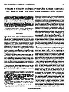
From these data we construct two datasets for double check. Each dataset contains two, well separated conceptual categories: respectively, network and metals, such as gold and silver for the former dataset and software and gold and silver for the latter one. The characteristics of each dataset are shown in Figure 2 together with the accuracy obtained by a 1-NN classifier on all the features.
Class One Class Two N. of features Accuracy dataset1 network gold and silver 6031 65.10% dataset2 software gold and silver 6104 58.69% Fig. 2. Characteristics of the data sets
We compare algorithm FRRW with other two algorithms for feature selection. The former is IGR [9]: it is based on Information Gain which in turn outperforms other measures for term selection, such as Mutual Information, χ2 , Term Strength as shown in [9]. The second one is a baseline selector, denoted by RanS, a simple random selection of the features that we introduce specifically for this work. Our experiments are conceived as follows. We run the three feature selection algorithms on each of the two datasets separately and obtain a ranking of the features by each method. From each of these rankings, we select the set of the top-ranked i features, with i that varies from 1 to 600. Thus the ability of the three algorithms to place at the top of the ranking the best features is checked. For each feature set of i features, chosen by the three methods, we project the dataset and let the same 1-NN classifier to predict
Algorithm 1 Feature Evaluation Framework 1: This procedure is for evaluation of unsupervised feature selection algorithms 2: FRRW(i), IGR(i): output vectors storing the accuracy of 1-NN on dataset D projected on top i features selected respectively by FRRW and IGR 3: RanS(i): output vector storing the average accuracy of 1-NN on a random selection of i features 4: for each data set D do 5: for i = 1 to 600 do 6: select top i features by FRRW, IGR 7: /* project D on the selected features */ 8: DF RRW (i) = ΠF RRW (i) (D) 9: DIGR(i) = ΠIGR(i) (D) 10: /* Determine 1-NN accuracy and store it in accuracy vector */ 11: FRRW[i] = 10-fold CV on DF RRW (i) using 1-NN 12: IGR[i] = 10-fold CV on DIGR(i) using 1-NN 13: /* determine average accuracy of 1-NN with RanS */ 14: tempAccuracy = 0; 15: for j = 1 to 50 step 1 do 16: DRanS(i) = ΠRanS(i) (D); 17: tempAccuracy=tempAccuracy + 10-fold CV on DRanS(i) using 1-NN 18: end for 19: RanS[i]= tempAccuracy/50 20: end for 21: end for
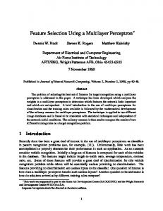
the class in a set of test instances (with 10 fold cross-validation) and store its accuracy. For RanS we perform 50 times the random selection of i features, for each value of i, and average the resulting classifier accuracy. Algorithm 1 sketches the algorithm we used for this evaluation. The accuracy of 1-NN resulting by the feature selection of the three methods is reported in Figure 3 and in Figure 4. In these figures we plot the accuracy achieved by the classifier on the instances respectively of dataset 1 and dataset 2 where the instances are represented by a subset of the features selected by each of the three methods. On the x axis we plot the number of selected features and on the y axis we plot the accuracy obtained by the classifier on the features selected by each of the three methods. In both of the two datasets our feature selection method induces the same behaviour of the classifier. In the first part of the graph the accuracy grows up to a certain level. After this maximum the accuracy decreases. This means that the most useful features are those ones at the top of the ranking. When we finish to consider in the set of selected features only these ”good features” and start to include the remaining ones, these latter ones introduce noise in the classification task. This is explained by the observed degradation of the classification accuracy. When we consider the other two methods, we can see that the accuracy not only is generally lower but it is also less stable when the number of features increases. It is clear that with FRRW the reachable accuracy is considerably higher (even higher than the accuracy obtained with the entire set of features). In particular, it is higher with FRRW even considering only a low
number of features. This behaviour perfectly fits our expectations: it means that the top-ranked features are also the most characteristic of the target concept, namely those ones that allow a good classification. On the other side, as we increase the number i of the features, the accuracy decreases (even if with FRRW it is still higher than with the other methods). This means that the ranking of the features induced by FRRW correctly places at the top of the list the features that contribute most to a correct classification. Instead, at the bottom of the list there are just those remaining features that are not useful for the characterization of the target concept, because they are the noisy ones.
4 Conclusion In this work we investigate the use of PageRank for feature selection. PageRank is a well-known graph-based ranking algorithm that performs a Random-Walk through the feature space and ranks the features according to their similarity with the greatest number of other features. We empirically demonstrate that this technique works well also in an unsupervised task (namely when no class is provided to the feature selection algorithm). We have shown that our method can rank features according to their classification utility, without considering the class information itself. This interesting result means our method can infer the intrinsic characteristics of the dataset, which is particularly useful in all those cases in which no class information is provided. As a future work we will want to investigate this method, of feature selection, for unsupervised learning such as the clustering task.
References 1. Baker L. D. and McCallum A. K., ‘Distributional clustering of words for text classication’, SIGIR98, (1998). 2. 7Sector data. http://www.cs.cmu.edu/afs/cs/project/hteo-20/www/data/bootstrappingie/. 3. Guyon I and Elisseeff A, ‘An introduction to variable and feature selection’, JMLR, 3, (2003). 4. Porter M.F., ‘An algorithm for suffix stripping’, Program, (1980). 5. James Norris, Markov Chains, Cambridge University Press, 1998. 6. Mihalcea R, ‘Unsupervised large-vocabulary word sense disambiguation with graph-based algorithms for sequence data labeling’, HLT/EMNLP05, (2005). 7. Brin S and Page L, ‘The anatomy of a large-scale hypertextual web search engine’, Computer Networks and ISDN Systems, 30, (1998). 8. Deng Cai Xiaofei He and C.F. Partha Niyogi, ‘Laplacian score for feature selection’, NIPS05, (2005). 9. Yang Y and Pedersen J O, ‘A comparative study on feature selection in text categorization’, ICML97, (1997). 10. Zheng Zhao and Huan Liu, ‘Semi-supervised feature selection via spectral analysis’, SDM07, (2007).
75 FRRW IGR RanS 70
Accuracy
65
60
55
50 0
100
200
300 Num of features
400
500
600
Fig. 3. Accuracy on dataset1. 75 FRRW IGR RanS 70
Accuracy
65
60
55
50 0
100
200
300 Num of features
400
Fig. 4. Accuracy on dataset2.
500
600