Using Python and ArcGIS Functions to Determine Net Radiation. (METRIC Application) ... 12/15/2014. Abstractâ The objective of this project is to automate procedures required .... Throughout the development and testing of this model, Lower.
Using Python and ArcGIS Functions to Determine Net Radiation (METRIC Application) Sulochan Dhungel, George Elliott, Mark Lewis, Brett Mooney CVEEN 7920 Hydroinformatics University of Utah 12/15/2014 Abstract— The objective of this project is to automate procedures required for calculating net radiation for use in the Mapping Evapo-Transpiration at high Resolution with Internalized Calibration (METRIC) model. This automation process is accomplished via various modules and scripts created in the Python coding language. In order to calculate ET via the METRIC model, the calculation of a myriad of parameters is required. This project’s output automates the calculation of a number of these parameters. Keywords—METRIC; Python; evapotranspiration; data extraction; Incoming Solar Radiation;
I.
INTRODUCTION
Evapotranspiration (ET) is the combined effects of surface and soil moisture evaporation with the water transpired from plants. On a global scale, a significant amount of water is lost to the processes of ET. In all continents apart from Antarctica, the volume of water lost to ET exceeds that of direct runoff in most river basins. Additionally, nearly 62% of all precipitation is lost to the processes of ET (Dingman, 2002). Therefore, quantifying ET is of great importance for water rights management, water resource planning, and water regulation. ET has been quantified either (1) by using point-based methods such as the ASCE Penman Monteith Equation (Allen et al., 2005), Blaney-Criddle (Allen and Pruitt, 1986) or (2) by using radiation balance approaches for an areal estimate. This project uses METRIC as the model for estimating ET. METRIC is a model developed at the University of Idaho, which uses satellite and weather data to calculate and map ET by estimating radiation balance (Allen et al., 2007). Terrestrial radiation balance uses incoming solar radiation, soil heat flux, and sensible heat flux for estimating latent heat flux, from which ET can be estimated. The energy balance equation is provided in Equation (1) and illustrated in Figure 1.
Figure 1. Estimating ET using radiation balance (Allen, 2005)
𝐸𝑇 = 𝑅𝑛 − 𝐺 − 𝐻
(1)
ET = Evapotranspiration estimated using Latent Heat Flux Rn = sum of net radiation (all incoming and outgoing short-wave and long-wave radiation at the ground surface) G=sensible heat flux conducted into the ground H=sensible heat flux convected to the air Due to limitations of time, only incoming solar radiation (a component of net radiation) was selected for this model development. Other parts of net radiation (Eq. 2) and estimates of G and H have also been excluded from this project due to time constraints of the academic semester. 𝑅𝑛 = 𝑅𝑆↓ − 𝛼𝑅𝑆↓ + 𝑅𝐿↓ − 𝑅𝐿↑ − (1 − 𝜀0 )
(2)
The goal of this project is to automate the procedure to estimate Rs.. Project Problem Statement Estimation of 𝑅𝑆↓ Incoming solar radiation is calculated using various empirical equations which have been modeled in METRIC. The complexity of this model is evident in Figure 2 provided below. METRIC was developed using an image processing software (ERDAS Imagine™), which requires an expensive commercial license as well as trained personnel. Thus, it is not a hands-off model. Modeling system of image processing software are quite complex, and those complexities are exacerbated when dynamic data is input into the model (i.e. individual days have unique data – the effect of solar radiation is unique for each hour of each day in the year). Therefore, automating the calculation of incoming solar radiation for use in MERIC not only requires automating scripts and processes, but also automation in extraction of required data.
spectral resolution. The model presented here is compatible with LandSat 4, 5, 7 and 8 products. 2.
Figure 2. Sub model for estimating solar radiation in mountains (developed for METRIC) (Allen, 2005)
Purpose The purpose of this project is to create a Python tool which automates data collection and subsequently computes Rs. Required Data In order to calculate ET via the METRIC model, satellite data (Landsat or MODIS) in conjunction with ground-based hourly or sub-hourly weather data is required. The calculation of incoming solar radiation is dependent upon the geographic location (latitude), relief of the location (elevation models), day of the year (position of the sun relative to earth), time of day, and atmospheric conditions, which govern the absorption/reflectance of incoming radiation. The sources of data required for calculation of these parameters are: 1.
Satellite Imagery (LandSat (LPSO, 2004))
Although the model described in this project does not currently use any of the reflectance data from satellite images, it does use the associated date and time data provided in the metadata file of the satellite image. Additionally, in order for METRIC to compute parameters of ET (such as albedo, reflected shortwave and long-wave radiation – which are not currently incorporated in the model), it does utilize reflectance data from satellite imagery.
Digital Elevation Model (DEM)
DEM data is required to compute slope and aspect, both of which determine the amount of radiation a specific location receives. In conjunction with weather data, DEM data is also used in the empirical calculation of atmospheric pressure, as well as water content in the atmosphere. Atmospheric pressure and water content in the atmosphere are surrogates for mass and optical depth of atmosphere. National Elevation Dataset (NED) (USGS, 2001) provides DEM data for various spatial resolution and file formats. Each 30-m resolution DEM file is provided at a one-degree latitude and longitude block. A FTP site is used to automate the download of DEMs (ftp://rockyftp.cr.usgs.gov/vdelivery/Datasets/Staged/NED/13) 3.
Weather Data
Hourly and sub-hourly weather data for vapor pressure is required for the model to compute water content in the atmosphere. Among various weather data sources, this project works with USBR AgriMet dataset (USBR, 2000). This dataset provides hourly and sub-hourly data for various hydrologic attributes. The AgriMet dataset provides data access via an appropriate URL. A URL template has been provided by USBR Agrimet site to assist in the automatic data extraction procedure. Data Management Data management was done using a digital file folder system. All required input files were put in a “Required Files” directory folder while intermediate files and associated final results were put in “Temp-Files” directory. Area of Study Throughout the development and testing of this model, Lower Yakima Watershed in Washington was selected as the area of interest (Figure 3). The Lower Yakima Watershed has one AgriMet site inside of its watershed boundaries.
LandSat data used in this project was downloaded using USGS earth explorer, a tool that aids in the downloading of satellite images. At the time of this study, to our knowledge, there were no web services available that could assist in the automatic extraction of satellite data. Recent developments in Google Earth Engine, which are still in trial phase, have shown potential in the direction of automatic extraction of satellite data. LandSat data provides moderate-resolution, land-remote sensing data, acquired for over four decades. Acquisition of LandSat data started with the Landsat 1 dataset and the most recent has been Landsat 8. With each subsequent LandSat dataset, there have been improvements in both spatial and
Figure 3. Pilot Watershed (Yakima)
II.
METHODS
The solar radiation estimation model developed in this study was accomplished by creating four distinct functionalities with Python. Additionally, multiple Python functions were created for each functionality. These four functionalities developed in this project is used to: 1. Prepare DEM. 2. Convert Greenwich Mean Time (GMT) to local date and time from downloaded Landsat Image metadata 3. Extract required weather data 4. Calculate incoming solar radiation These four methods are described below in detail. Figure 5. Python model for extraction of DEM
1. Preparation of DEM Preparation of DEM data for the model involves downloading DEM for the required area of interest, creating a mosaic of the areas to form a single DEM file, and subsequently clipping out the shape or image file (Figure 4). This same procedure was employed to automate the DEM preparation tasks required of the METRIC model. Figure 5 is a flowchart which summarizes the procedure required to prepare the DEM files.
These DEM files were downloaded in zipped file format. The Python Unzip module was used to systematically unzip the required DEM files into folders. These unzipped files were then mosaicked using the Python arcPy module, developed by ArcGIS, which resulted in a large mosaicked DEM, which contained the image or shape file of interest. The area of interest was then clipped from this DEM mosaic using the clipping functionality of the Python arcPy module. The final result was a clipped DEM file ready to be used by the METRIC model. A screenshot of the DEM preparation model is presented in Figure 6. 2. Conversion of GMT to local date and time from LandSat Image
Figure 4. Process to prepare DEM for METRIC
The METRIC model uses date and time data of satellite images to compute incoming solar radiation. Furthermore, a number of additional parameters required to compute incoming solar radiation, such as hour angle, angle of declination, and relative earth-sun distance, also require local date and time. However, satellite date and time information is provided in GMT format. Hence, to automate calculations for METRIC, a function to convert GMT satellite data to local date time, based solely on image metadata was required.
First, the extent of the image file or watershed shape file was determined. Extents of a Landsat image file are provided in the associated metadata file while the Python shapefile module was used to determine extents of watershed shape file. The Python os module was used for discovering metadata file from the directory and extracting image extents. This extent was used to prepare the list of required DEM files. An ftp site operated by the USGS was created in order to provide easier access to automatically download DEM data. (ftp://rockyftp.cr.usgs.gov/vdelivery/Datasets/Staged/NED/13)
In addition to the conversion of GMT to local date and time, relevant time zone information as well as Daylight Savings (DLS) time had to be accounted for. The time of acquisition of satellite images is provided as the GMT of the center of the image. Hence, the major steps in conversion of GMT to local date and time involves the calculation of center of image, identification of the time zone the center lies on, and the determination of daylight savings, if applicable. An overview of this process is presented in Figure 7 and steps are outlined in Figure 8.
Figure 8. Use of python to get local date and time from GMT of scene center
First, latitude and longitude of the image center are calculated using the extents of the satellite image. The latitude and longitude are converted into a point shape file using the Python shapefile module. The Spatial join function from the arcPy module is then used to join the time zone shape file (which contains GMT offset data along with DLS data) with the newly created point shape file. This results in a point which has a GMT offset and DLS data. By utilizing the associated metadata file, the local date is then extracted which, in turn is used to determine if DLS applies for the particular date. Thus, the local date-time is calculated using GMT, GMT offset, and DLS. 3. Extraction of Weather Data
Figure 6. Screenshot of the model to prepare DEM
One of the inputs METRIC requires is that of hourly or subhourly weather data provided by a land-based weather site. The preparation of this weather data for METRIC involves the selection of weather sites inside a given watershed. If there are no weather sites present inside the boundaries of the selected watershed, sites close to the watershed are selected via interpolation methods such as Theissen polygons. Once an appropriate weather site is selected, the calculation of local date time and the extraction of weather data is possible. The time information of the image for each site is presented in GMT for the given date and time. Additionally, multiple time zones and variances in DLS may vary between weather sites, but the sites still reside within the same image or watershed. An overview of the process is presented in Figure 9 and the procedure followed by the model is presented in Figure 10.
Figure 7. Conversion of GMT of scene center to Local Date Time
Thiessen polygons are first created for AgriMet sites (using the Python arcPy module) which are then clipped (using the Python shapefile module) and the watershed boundaries are then used to select weather stations in the clipped watershed area. All Theissen polygons might not accurately represent the weather condition inside the watershed due to differences in location and elevation of sites; therefore, the selection of weather sites might have to be done by careful investigation of
the related site. One example would be in the instance where there is large difference in elevation between two weather stations, which would cause large differences in weather patterns despite close proximity of weather stations. Once appropriate weather sites are selected, the satellite GMT data is converted into local date and time (as explained in subsection (2) above). Weather data for selected sites at the specified date and time is then downloaded from AgriMet. AgriMet provides time data using a URL with a specific template, facilitating the automatic download of weather data. In the link, http://www.usbr.gov/pnbin/webarccsv.pl?station=HRHW&year=2015&month=1&day =1&year=2012&month=1&day=1&pcode=MM&pcode=TA HRWH represents the station identification, the time is represented by year, month and day, selecting the start and end times of the relevant data. The pcode represents the variable identification. This weather data is then downloaded and aggregated for each site used in the model.
4.
Calculation of incoming solar radiation
The results of the procedures described above are used in the final calculation of incoming solar radiation. The calculation of incoming solar radiation requires the calculation of slope, aspect and latitude raster using DEM data, hour angle, angle of declination and relative earth-sun distance using local date time, all of which are then used to compute the solar incidence angle. This solar incidence angle is then used with broad-band transmissivity computed using elevation-derived atmospheric pressure and water content in the atmosphere. The calculation of these parameters was accomplished with the spatial analyst tool within the Python arcPy module. The major steps in calculation of solar radiation are summarized in Figure 11.
Figure 9. Selection of sites and extraction of weather data
Figure 11. Calculation of Solar Radiation
Figure 10. Use of Python to prepare weather data
Slope and aspect are initially calculated from DEM data using the Python arcPy module. Aspect in METRIC is expressed from –π to + π. Hence, the Python numPy module was used to transform the arcPy aspect data into aspect data for use with METRIC. There are no functions in arcPy to compute a latitude raster. Therfore, the Numpy module was utilized in order to compute the required latitude raster. Using local date and time information, the day of year along with angle of declination, hour angle, and relative earth-sun distance was computed. All of these individual raster data sets were brought together and incoming solar radiation was then computed as shown in Figure 12.
III.
RESULTS
The result of this project is a working model, which can calculate incoming solar radiation from a LandSat image and a watershed shapefile. Most functions created during development of the model are standalone functions which can be used independently. IV.
Figure 12. Incoming Solar Radiation
Supporting Python Functionalities: During the development of this model, some additional Python functions were developed. 1.
Split and Combine Raster Due to large size of some image data sets, some computer systems struggled with computations and eventually crashed. Therefore, this tool was created to split a large raster into smaller rasters. Analysis was then performed on these small rasters. The smaller rasters are subsequently identified and indexed during the splitting process allowing Python to reassemble the raster images in the correct order.
2.
Calculate Latitude Raster Prior to ArcGis 10.1, the latitude raster could be created using built-in GIS functions. This function has been discontinued in ArcGis, therefore, this tool helps to acquire the latitude raster using the associated DEM raster. NumPy and arcPy modules were also used in this tool.
3.
Compute Daylight Savings This function determines start and end of daylight savings time based on user input of the year. Daylight savings were calculated based on start on the second Sunday of March at 2:00 am and end on the second Sunday in November at 2:00 am each year.
4.
Get Extents This Python tool was created in order to acquire the extents of raster or vector data. Python arcPy module was used for raster data sets and Python shape file module was used for vector data sets. The inputs were file names of raster or vector files. The outputs were the maximum and minimum latitude and longitude values of the extent. Special Case: For satellite (LandSat data), extents were extracted from the associated metadata file.
CONCLUSIONS AND FUTURE EFFORT
This project demonstrated the use of Python to extract data from web servers, process it for the final use in a model, and analyze it using packages and modules from various sources. This project also demonstrated the use of Python in analyzing various aspects of the model individually and ultimately, combining the relevant data together, creating a simpler, and more flexible model. As each component function of the model has been developed as an individual function, changing the components of model with new and enhanced functions is simplified. Furthermore, Python is a widely-used, free programming software language. New functions developed by other users can be integrated into the existing model to make it better. Future efforts will be made to finish the entire model, calculating the remaining parameters required by the METRIC model, resulting in the complete computation of ET. Additional functions will also be added, such as the automatic retrieval of a csv files, so that this model can be employed where no AgriMet sites are available. Furthermore, with the development of tools such as Google Earth Engine, the automatic download of satellite data will be enhanced. Finally, a graphical user interface for the model will also be developed. REFERENCES Allen R, Pruitt W. 1986. Rational use of the fao blaney‐ criddle formula. Journal of Irrigation and Drainage Engineering 112139-155. DOI: doi:10.1061/(ASCE)0733-9437(1986)112:2(139). Allen R, Tasumi M, Morse A, Trezza R, Wright J, Bastiaanssen W, Kramber W, Lorite I, Robison C. 2007. Satellite-based energy balance for mapping evapotranspiration with internalized calibration (metric)—applications. Journal of Irrigation and Drainage Engineering 133395-406. DOI: doi:10.1061/(ASCE)0733-9437(2007)133:4(395). Allen RG 2005, Evapotranspiration from remote sensing using surface energy balance workshop, edited, Ft. Collins, CO. Allen RG, Walter IA, Elliot RL, Howell TA (Eds.) 2005, Asce standardized reference evapotranspiration equation, 216 pp., American Society of Civil Engineers. Dingman SL. 2002. Physical hydrology. Prentice Hall
LPSO 2004, Landsat 7 science data users handbook, http://landsat.usgs.gov/using_Landsat_7_data.php, MD, (updated USBR 2000, Agrimet: Pacific northwest cooperative agricultural weather network, edited. USGS 2001, Usgs national elevation dataset, edited, EROS Data Center.