Using routine hydrographic sections for estimating the parameters ...

sm69n4435

18/11/05

08:19

Página 435

SCI. MAR., 69 (4): 435-449

SCIENTIA MARINA

2005

Using routine hydrographic sections for estimating the parameters needed for Optimal Statistical Interpolation. Application to the northern Alboran Sea* MANUEL VARGAS-YÁÑEZ, FLORIAN GARIVIER, OLIVIER PIRRA and M. GARCÍA-MARTÍNEZ Instituto Español de Oceanografía, C.O. Málaga (Fuengirola), Puerto Pesquero de Fuengirola s/n, 29640 Fuengirola, Málaga, Spain. E-mail: [email protected]

SUMMARY: Optimal Statistical Interpolation is widely applied in the analysis of oceanographic data. This technique requires knowing some statistics of the analysed fields such as the covariance function and the noise to signal ratio. The different parameters needed should be obtained from historical data sets, but, in contrast with the case of meteorology, these data sets are not frequently available for oceanographic purposes. Here we show that using routine hydrographic samplings can provide a good estimate of the statistics needed to perform an Optimal Statistical Interpolation. These data sets allow the covariance function to be estimated between two points with different horizontal and vertical coordinates taking into account the possible lack of homogeneity and isotropy which is rarely considered. This also allows us to accomplish a three-dimensional analysis of hydrographic data, which yields smaller analysis errors than a traditional two-dimensional analysis would. Keywords: Optimal Statistical Interpolation, time series, routine sampling, Alboran Sea, covariance function. RESUMEN: USO DE MUESTREOS HIDROLÓGICOS SISTEMÁTICOS PARA LA ESTIMACIÓN DE LOS ESTADÍSTICOS NECESARIOS EN TÉCNICAS DE INTERPOLACIÓN ÓPTIMA. APLICACIÓN AL SECTOR NORTE DEL MAR DE ALBORÁN. – La interpolación óptima es ampliamente aplicada al análisis de datos oceanográficos. Esta técnica requiere el conocimiento de algunos estadísticos de los campos analizados, como la función de covarianza o la razón ruido-señal. Los distintos parámetros necesarios deberían obtenerse a partir de series históricas de datos, sin embargo, al contrario de lo que ocurre en meteorología, esto no es posible en la mayor parte de los casos cuando esta técnica es aplicada a datos oceanográficos. En este trabajo se muestra que el uso de muestreos hidrológicos rutinarios puede proporcionar una buena estimación de los estadísticos necesarios en interpolación óptima. Estos datos permiten la obtención de la función de covarianza entre dos puntos cualesquiera con diferentes coordenadas verticales y horizontales, tomando en consideración la posible falta de homogeneidad o isotropía. Esto permite realizar un análisis tridimensional de los datos que proporciona valores de los errores del análisis más bajos que los producidos por la interpolación bidimensional frecuentemente empleada. Palabras clave: Interpolación Óptima, series temporales, muestreo sistemático, Mar de Alboran, función de covarianza.

INTRODUCTION A significant component of our present knowledge about the water mass properties and its general circulation comes from hydrographic cruises and *Received September 6, 2004. Accepted April 29, 2005.

from data obtained from ships of opportunity. Traditionally, these surveys were accomplished by means of bottle samples or XBTs and CTDs obtained at a set of predefined stations. More recently we have begun to obtain hydrographic data from profiling floats which drift freely with currents at a fixed depth. Studying these data requires contouring

ESTIMATION OF PARAMETERS FOR OPTIMAL STATISTICAL INTERPOLATION 435

sm69n4435

18/11/05

08:19

Página 436

different variables as well as computing derived fields such as geostrophic velocity, vorticity, etc., which involves computing certain variables by means of finite differences. For this purpose, the observed data are interpolated onto a regular grid. Several methods are used for interpolating oceanographic data (see Thiébaux and Pedder, 1987 for a review), including distance-weighting schemes and Optimal Statistical Interpolation (OSI hereafter). OSI was originally developed by meteorologists (Gandin, 1963), and first described in an oceanographic context by Bretherton et al. (1976), although it was referred to as objective analysis. It has several advantages over traditional distance-weighting methods as it takes into account the correlation between nearby observations, allows the analysis error to be estimated and considers the observational errors, smoothing the interpolated field. Another advantage of OSI is that univariate analysis can be easily extended to multivariate analysis as long as the cross correlation between different variables is known (Gomis et al., 2001). The OSI is optimal in a statistical sense (see Section 3), but requires knowing the covariance function of the analysed field as well as the ratio of the error variance to the signal variance. Another characteristic of this method is that it is applied to increment fields, the differences between the observed fields and a certain drift, background or first guess. As pointed out by Gomis et al. (2001), “Both the statistical mean field and correlations between increment pairs should in principle be derived from historical data sets”. During recent decades several oceanographic atlases have appeared, such as that by Levitus et al. (1994), or for the specific case of the Mediterranean sea, MEDATLAS (1997). These atlases provide temperature and salinity mean values which can be used for calculating increments from the observed values, but they do not allow us to obtain the covariance function or the noise to signal ratio. In almost all of the cases, these parameters are estimated from a single oceanographic cruise. Freeland and Gould (1976), estimated the longitudinal and the transverse velocity correlation function from neutrally buoyant floats, assuming isotropy, stationarity and homogeneity. Robinson et al. (1987), used an homogeneous, isotropic and stationary correlation function to study the mesoscale fields in the Eastern Mediterranean. Carter and Robinson (1987), obtained a non-isotropic and time dependent correlation function from both a XBT survey and from an 436 M. VARGAS-YÁÑEZ et al.

array of moored current meters, and Mariano and Brown (1992), considered the possible heterogeneous character of the correlation function dividing the interpolation domain into several spatial and time bins. In most of the cases using a single survey or short length time series implies that several assumptions have to be made in a subjective way and in some cases some parameters that are needed to define the covariance function are chosen in a trial and error form. Nevertheless, the advantages of this objective analysis method lie in the explicit form of the assumptions, the repeatability of the operations and the ability to obtain error fields, but as stated by Roemmich (1983), “with limited data, human judgement cannot be removed from the problem. From that standpoint, linear estimation is no different from or better than, say, hand-contouring”. Repeated standard hydrographic sections can be used as observations similar to those from meteorological stations allowing us to obtain accurate mean or climatological values as well as correlations between pairs of stations. The purpose of this work is threefold: 1) We want to illustrate the potential use of these periodic surveys for calculating background fields, covariances between different stations and noise to signal ratios in a similar way to that used in meteorology. These results could also be extended to the recent use of profiling floats in the Argo project. 2) Estimating the statistics of different variables will allow us to check several hypotheses usually assumed in the OSI of oceanographic data, such as isotropy and homogeneity. 3) Finally, we address the problem of finding a covariance function that allows a fully three-dimensional OSI, combining the horizontal and vertical directions and improving previous attempts to find a covariance function for the interpolation of vertical hydrographic sections. Values of these functions and the different parameters involved are presented for the specific case of the Alboran Sea. DATA Ecomálaga is a multidisciplinary project aimed at studying environmental conditions within the continental shelf of the area surrounding Málaga Bay in the northern riparian of the Alboran Sea (Fig. 1). From October 1992 to the present, three transects perpendicular to the coast have been revisited four times a year. These transects extend from Cape Pino, Málaga and Vélez and each com-

sm69n4435

18/11/05

08:19

Página 437

FIG. 1. – Position of the stations sampled in Ecomálaga project. Stations with circles and labelled with letters P, M and V and numbers 1, 2, 3 are those stations sampled since 1992 and used in estimating the correlation and covariance functions. The rest of the stations (crosses) are those sampled since 2000 and have not been used for statistics estimations; nevertheless, they have been used in Results for a comparison between 2D and 3D interpolation schemes. Arrows show a schematic of the circulation in the upper layer of this area.

Freeland and Gould, 1976; Roemmich, 1983; Robinson et al., 1987; Carter and Robinson, 1987; Thiébaux and Pedder, 1987; Lorenc, 1991; Fukumori and Wunsch, 1992; Mariano and Brown, 1992; Pedder, 1993; Gomis et al., 2001). Here we present a brief summary. OSI is applied to increment fields (θ) which represent the difference between the observed variable (φ) at a space point r and a drift or background value at the same point (µ). It is also assumed that the observations and therefore the increments have a certain error (ε), which represents not only instrumental error but also the part of the variance of the increment field which is associated with those wavenumbers and frequencies not resolved by the data. We consider a set of n observations which can be decomposed as φi=µi+θi+εi. The problem addressed is to estimate the increment field at a grid point “g” as a linear combination of the n observed increments (which contain the error term):

prise three stations. These stations are identified by the letter, P for the Cape Pino transect, M for Málaga and V for Vélez, and by a number, 1 for the most inshore station, 2 for the intermediate one, and 3 for the offshore station. The three inshore stations are over a bottom depth of 25 m. Intermediate stations have a depth of 75 m in the cases of M2 and V2 and 110 for P2. The offshore stations have depths of 540, 200 and 300m for P3, M3 and V3 respectively. Here we analyse time series to a maximum depth of 200m. At each station a CTD cast is made. We will analyse temperature, salinity and specific volume anomaly (svan hereafter) from 5 to 200m at an interval of 5m. Time series analysed extend from October 1992 to October 2003 (included). There were a total of 45 cruises, but the time series analysed have some gaps and the final data set has a total number of 41 measurements for each station and depth. Since the year 2000, three more transects (F, T and R in Fig. 1) have been added, as well as two more stations on the Málaga transect and one more on the Vélez transect. Nevertheless, as these time series are not long enough, we will not consider them when estimating mean values and correlations.

being ϕi=θi+εi. If wg is a column vector containing the n weights in (1) and ϕ is a vector with the n observed increments, we can write (1) in matrix form θˆg = wTgϕ, where ( )T denotes transposition and the hat denotes estimation. The analysis error will be the difference between the true increment and the estimated increment. OSI is optimal in the sense that it minimises the variance of the analysis error 〈(θg – θˆg) 2〉 where the brackets denote expectation or average over an infinite ensemble of independent realisations of the process. The solution to the minimisation problem is wg = A-1Cg, êg = C Tg A-1ϕ and the error variance is σ 2s (1C Tg A-1Cg). Where σ2s is the signal variance, CTg = (Cgl,......,C gn) denotes the correlation between the grid point “g” and the n observation points and A=C+γI. C is a nxn matrix where the Cij element is the correlation between the observation points “i” and “j”, I is the identity matrix and γ is the noise to signal ratio σ 2ε /σ 2s.

OPTIMAL STATISTICAL INTERPOLATION

RESULTS

OSI was first developed by meteorologists (Gandin, 1963), but since then, many papers have applied it to oceanographic data (see for instance among many others Bretherton et al., 1976;

In most of the oceanographic applications where a fully three-dimensional (3D) data set is available, (a typical CTD cruise) there are several limitations to applying the OSI method. The first one is that the

n

θˆg = ∑ w g ,iϕ i

(1)

i=1

ESTIMATION OF PARAMETERS FOR OPTIMAL STATISTICAL INTERPOLATION 437

18/11/05

08:19

Página 438

salinity derivative (m-1 )

salinity 36.8

37.2

37.6

38

0

38.4

0

0

-40

-40

depth (m)

depth (m)

36.4

-80

-120

-160

0.005

0.015

0.02

0.025

0.16

0.2

-80

-120

d)

-200 12

14

16

18

0

20

0.04

36.8

37.2

37.6

38

0

38.4 0

-40

-40

depth (m)

0

-80

-120

b)

-160

0.12

salinity derivative (m-1)

salinity 36.4

0.08

temperature derivative (ºCm-1 )

temperature (ºC)

depth (m)

0.01

-160

a)

-200

0.005

0.01

0.015

0.02

0.025

-80

-120

e)

-160

-200

-200 12

14

16

18

0

20

salinity 36.4

36.8

37.2

37.6

38

0

38.4 0

-40

-40

depth (m)

0

-80

-120

c)

-160

0.04

0.08

0.12

0.16

temperature derivative (ºCm-1 ) salinity derivative (m-1 )

temperature (ºC)

depth (m)

sm69n4435

0.005

0.01

0.015

0.02

0.025

0.16

0.2

-80

-120

f)

-160

-200

-200 12

14

16

18

temperature (ºC)

20

0

0.04

0.08

0.12

temperature derivative (ºCm-1 )

Fig. 2. – Temperature (solid line) and salinity (dashed lines) mean profiles at P3, M3 and V3 (a, b and c respectively). In all the cases we have obtained a profile for each season of the year. Squares correspond to summer (July-September), crosses to autumn (October-December), triangles to winter (January-March) and circles to spring (April-June). Figures 2d, e, f . Vertical derivatives of temperature and salinity. Line and symbol criteria are the same as in Figures a, b, c.

438 M. VARGAS-YÁÑEZ et al.

sm69n4435

18/11/05

08:19

Página 439

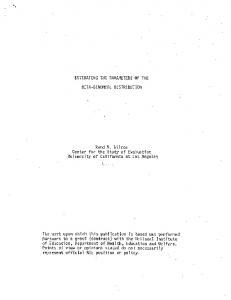
3D field is analysed by means of the 2D analysis of successive horizontal surfaces at different depths or pressure levels. This method does not take into account the information provided by neighbouring points at different horizontal levels. The reason for this simplification is that the correlation function is usually assumed to be isotropic and obviously this does not hold when both the horizontal and vertical directions are involved in the analysis. When a vertical hydrographic section is analysed this problem is solved by analysing and mapping the data for each single depth (1D analysis, Lavín, 1999), or by introducing a scale factor relating the horizontal and vertical distances (Roemmich, 1983). Nevertheless the covariance function used in these cases implies some assumptions that are not appropriate as we will show in the following sections. Estimating the background or drift field In many cases there are no climatological data sets for estimating the background mean fields or the needed covariance functions. The mean field is sometimes estimated by fitting a low-order polynomial to the data. In our case we can get the mean values by averaging all the available data for each station and depth. The average takes into account the possible existence of seasonal cycles and different averages are accomplished for each season of the year. Once these climatological profiles are obtained, we derive the increments by subtracting from each profile the climatological profile corresponding to its location and the corresponding season of the year. Figures 2a, b and c show the seasonal temperature and salinity profiles for the P3, M3 and V3 stations. Horizontal correlations The mean values show some onshore-offshore and west to east gradients mainly due to the distribution of Atlantic and Mediterranean waters and to the sloping of isotherms and isohalines due to the Atlantic current flowing to the south of our study area (not shown). It is usually assumed that the mean field over a horizontal section captures most of the anisotropy of the field and so the increment correlations depend only on the distance. The procedure in meteorology is to compute the correlation between the increments at different pairs of stations and to represent these correlations as a function of the distance. Figures 3a-f show the correlation

between all the pairs of stations available at 5, 25, 50, 75, 100 and 200 m. In all the figures we include the correlation for temperature (triangles), salinity (circles) and svan (open squares). The number of stations available for calculating correlations decreases with depth. This increases the errors and makes the decrease in correlation with distance more difficult to see clearly for the 100 and 200m cases. From 5 to 75 m this behaviour is clear. We propose two different functions for modelling the decrease of correlation with distance, a gaussian function and an exponential one: −

ρ( r ) = e

r2 2 L2x

−

ρ( r ) = e

r Lx

,

where r is the distance between two points for a fixed horizontal surface. Theoretically the correlation for r=0 is 1. Nevertheless the correlations estimated do not tend to unity as the distance approaches zero, or in our case, to the minimum separation between stations. This is due to the observational noise. The noise at different locations is independent and thus cancels when the covariance is estimated. On the other hand, the covariance estimate is divided by the variance of the increment field, and in this case the variance of the noise is retained. Instead of the functions above we fit functions of the form −

ρ ( r ) = R0e

r2 2 L2x

−

and ρ ( r ) = R0e

r Lx

(Thiébaux and Pedder, 1987). In both cases we estimate two parameters from the fit, R0 and the decay length scale Lx. The fit parameter R0 provides an estimation of

σ s2 σ s2 + σε2 and the noise to signal ratio can be calculated as 1 −1 . R0 If the fit is made for the covariance function then we could estimate the decay length scale and the observed increment variance σ 2 = σ 2s + σ 2ε . We used both the gaussian and the exponential function to model the correlation and covariance dependence with distance. Using the mean squared error (mse) as criterion, the exponential function provides a better fit to the sampled correlation and covariance functions, nevertheless, the differences

γ=

ESTIMATION OF PARAMETERS FOR OPTIMAL STATISTICAL INTERPOLATION 439

sm69n4435

18/11/05

08:19

Página 440

Fig. 3. – Correlation versus distance for 5, 25, 50, 75, 100 and 200 db (a, b, c, d, e and f respectively). In all the figures we include the correlation for temperature (triangles), salinity (circles) and svan (open squares) and the fit using a function of the form −

R0e

r2 2 L2x

.The solid line is the fit for temperature, the dashed line for salinity and broken line for svan.

440 M. VARGAS-YÁÑEZ et al.

sm69n4435

18/11/05

08:19

Página 441

are not very large (mse for the exponential fit is typically 10% lower than the mse for the gaussian one). The exponential model also provides a lower noise to signal ratio. On the other hand, the exponential function derivative is discontinuous at the origin. This is not a major problem for univariate analysis, but would not be a suitable correlation function in the case of multivariate analysis where some cross-correlation functions are related through their first derivatives. For this reason we will use the gaussian function in the interpolations performed in Section 4. We have also included the gaussian fit in Figure 3. Nevertheless, we provide the fit parameters for both correlation functions in Table 1 and in Figure 4. They show clearly the decrease of the variance with depth for temperature and svan. To find the functional dependence of the total variance with depth we fit exponential functions to the temperature and svan variances. The results are σ 2 ( z ) = 1.74 e

−

z 40 º C 2

for temperature and σ 2 ( z ) = 2.64 e

−

z 42 (10−12 m 3kg−1 ) 2

for svan, where z is the depth in meters. For the case of salinity, the variance seems to increase from the surface to a depth of around 40 m, and then it decreases with depth to the maximum depth sampled. The variance is a measure of the range of variability of the variable. It is reasonable to accept that a variable will change in a wider range in those areas affected by stronger gradients. Upward and downward movements of the water masses will cause larger deviations from the mean in those areas affected by strong vertical gradients. In the same way changes in the slope of the isohalines due to changes in the strength or position of the main currents will have a similar effect. Figures 2d, e and f show the vertical derivative of temperature and salinity at the three offshore stations. In all the cases, the maximum temperature vertical gradients are at the sea surface decreasing with depth. The only exception is in winter when the maximum derivative could be in the subsurface, although this is not clear on the plot. The reason is obviously that the temperature is dominated by the seasonal thermocline developed from spring to autumn and broken in winter when the permanent thermocline associated with the Atlantic and Mediterranean

TABLE 1. – Different parameters representing the covariance and correlation function for temperature, salinity and svan at different depths. In all the cases the first value is obtained by fitting an exponential function to the covariances or correlations represented versus distance while the second value corresponds to the gaussian fit (see text, Section 4.2). temperature/depth σ 2 (ºC2) 5 25 50 75 100 200 average salinity/depth 5 25 50 75 100 200 average svan/depth 5 25 50 75 100 200 average

R0

L(km)

γ

2.24/2.08 1.48/1.37 0.41/0.37 0.18/0.16 0.08/0.08 0.02/0.02

0.96/0.89 0.89/0.83 0.94/0.85 0.91/0.81 0.92/0.87 0.99/0.97 0.94/0.87

144/74 148/76 80/54 71/52 103/60 212*/85 126/67

0.05/0.12 0.12/0.21 0.06/0.17 0.1/0.24 0.09/0.16 0.01/0.03 0.07/0.16

σ2

R0

L(km)

0.07/0.06 1.05*/0.83 0.09/0.08 0.92/0.8 0.09/0.08 0.95/0.86 0.05/0.04 0.86/0.76 0.02/0.013 0.82/0.69 0.003/0.002 0.93/0.86 0.94/0.8

σ 2 (10-12m3/kg)2

R0

2.2/1.96 1.9/1.69 1.0/0.93 0.5/0.44 0.2/0.15 0.03/0.026

0.96/0.87 0.91/0.83 0.94/0.86 0.86/0.74 0.84/0.72 0.94/0.88 0.92/0.82

γ

35/35 -0.05*/0.2 68/51 0.09/0.26 84/55 0.06/0.16 76/56 0.2/0.32 40/39 0.2/0.45 89/59 0.08/0.17 65/49 0.09/0.26 L(km) 107/63 118/68 84/55 67/52 45/41 100/61 87/57

γ 0.04/0.15 0.1/0.2 0.06/0.17 0.16/0.35 0.19/0.38 0.06/0.14 0.10/0.23

* this value, as well as the R0>1, makes no sense and is an artefact of the fit.

waters has a more important role. For salinity, the seasonal effects which probably exist (see VargasYáñez et al., 2005), are of second order importance with respect to the permanent halocline which governs the vertical gradients. For all seasons and for all three stations the maximum vertical gradient of salinity occurs around 46m depth. This is consistent with the variations of salinity variance with depth. In this case we model this functional dependence as 2

σ ( z ) = 0.11e

−

z − 46 40

We also modelled the decrease of the variance with depth using a gaussian function but the results were considerably worse. For the other two parameters involved in the correlation and covariance function, Lx and γ, no clear depth dependence is found and it is more likely that these parameters do not vary systematically with depth. As the time series grows in length, either a clear pattern should evolve, or else the amplitude of these random fluctuations should decrease.

ESTIMATION OF PARAMETERS FOR OPTIMAL STATISTICAL INTERPOLATION 441

18/11/05

08:19

Página 442

temperature 2.5

800

0.2

1.5

600

0.15

1

400

0.5

200

0.05

0

0

500

0.5

variance (ºC 2)

2

a)

0 0

40

80

120

160

0.1

noise/signal ratio

0.25

Lx (km)

1000

200

salinity 0.12

0.4 0.3 300

Lx (km)

variance

400

0.04

0.2 0.1

200

noise/signal ratio

b) 0.08

0 0 0

40

80

120

160

100

-0.1

600

0.4

200

specific volume anomaly 3

500 400

0.3

300

0.2

1 200 100

0 0

40

80

120

160

0.1

noise/signal ratio

c) 2

Lx (km)

variance (10-13 m6/kg2)

sm69n4435

0

200

depth (m)

FIG. 4. – Variance obtained for different depths (5, 25, 50, 75, 100 and 200 db): We obtained the covariance as a function of the distance (in the same way that we did for correlation in Fig. 3) and then we fit both a gaussian −

r

r

− ) and an exponential function( 2 Lx ). σ e σ e Triangles represent the parameter of the fit σ 2 for the different depths analysed. The same fit was applied to the correlation function and from it we obtained R0 (see the text). Squares are the noise to signal ratio for each depth, calculated from R0, and the decay length scale is represented by circles. Filled symbols correspond to the gaussian fit and open symbols to the exponential one. The thick solid line is the theoretical depth dependence of the variance presented in Section 4.2, and crosses represent the variance as a function of depth obtained from the covariance estimation for a fixed station and different depths and then setting z1=z2 (see text, Section 4.3). Panels a, b and c show the same calculations for temperature, salinity and svan respectively.

(

2

2 L2x

Vertical correlations As already stated, when we deal with a vertical section or we wish to analyse a 3D field, we have two alternatives: One is to analyse the different depth levels separately and the other is to consider the covariance between two points with position vectors r1 and r2 such as γ ( r1 , r2 ) = σ 2e

−

r2 2 L2x

−

∆z 2 2 L2z

(Roemmich, 1983), where r is the horizontal distance between the two points (we assume isotropy in 442 M. VARGAS-YÁÑEZ et al.

the horizontal) and ∆z is the vertical distance. The decay length scales Lx and Lz account for the anisotropy between the horizontal and vertical directions. It is easy to see from the results in Section 4.2 that this function does not represent the true statistics of the oceanographic variables analysed above. First, let’s consider that for r1=r2, r= ∆z=0, this expression provides the same variance regardless of the depth. For two pairs of points separated by the same horizontal distance (r), but located at different depths, this function does not take into account the dependence of the variance on depth. If we consider pairs of points with the same horizontal coordinate (r=0) but different depths, this expression indicates that the covariance between the points depends on the vertical separation but not on the depth of the two points. Figure 5 shows the covariance between pairs of points with the same horizontal coordinate (we fix the station) as a function of the depth difference of the two points. We have repeated these calculations changing the depth of the initial point, in other words, the curve labelled ‘5 m’ represents the covariance between a point located at 5 m depth and all the points with the same horizontal coordinate and depths from 5 to 200 m as a function of the depth difference. The curve labelled with 25 m is the covariance between a point at 25 m depth and all the points with depths ranging between 25 and 200 m, expressed as a function of the depth difference, etc. Figures 5a, b and c show that it is not realistic to assume that the covariance function depends only on the depth difference. According to Figure 5 we could say that for two points with vertical coordinates z1 and z2, it depends on z1 and ∆z, or in a more simple form that it depends on both z1 and z2, and the homogeneity hypothesis is clearly not acceptable for the vertical dependence. Let’s consider a certain station (horizontal coordinate fixed). We estimate from the increment time series the covariance for all the possible pairs of values z1 and z2. We repeat these calculations for the three offshore stations where a more extensive description of the covariance depth dependence is possible. Results for P3, M3 and V3 are very similar confirming that the covariance function is homogeneous in the horizontal direction, so we averaged results for the three stations. Figure 6 shows the isolines for constant covariance. It is important to note that the covariances for z1=z2 represent the variance as a function of depth. The difference between this and the calculations in Figure 4 is that here we have

18/11/05

08:19

Página 443

a continuous description of the water column instead of 6 discrete levels, but we only consider the results from the most offshore stations instead of using all the available stations at a given depth level. The new dependence of variance with depth has been included in Figure 4 as crosses and these results are consistent with the previous ones. Visual inspection of Figure 6 shows that the covariance is roughly constant on ellipses decreasing as the semi-axis increases. That is, we treat the covariance as if it takes the form

2.5

temperature covariance

covariance (ºC 2)

2

5m 25m 50m 75m 100m

1.5

1

0.5

a) f(α 1 z12 + α 2 z22 +α 3 z 1 z2),

0 0

40

0.1

80 120 ∆z (m)

160

200

where f is a monotonic decreasing function. We propose that the covariance decreases as a gaussian function, cov(z 1 z2) = be – (α z + α z +α z z ) or as an exponential one, 2

1

cov( z1 , z 2 ) = βe covariance

1

2

2

2

3

1

2

salinity covariance

0.08

− (α1 z12 +α 2 z 22 +α 3 z1 z 2 )

0.06 0.04

For the gaussian model an intuitive interpretation is easy. In the case that a1=a2 we can write

b)

∆z and ∆z z2 = z + 2 2 where we assume, without losing generality, that we are in the case z1 = z −

0.02 0

z1