Using Static Flow Patterns in Time-Staged ... - Princeton University

Using Static Flow Patterns in Time-Staged Resource Allocation Problems

Arun Marar Warren B. Powell Hugo P. Sim˜ao

Department of Operations Research and Financial Engineering, Princeton University, Princeton, NJ 08544

September 6, 2006

Abstract

We address the problem of combining a cost-based simulation model, which makes decisions over time by minimizing a cost model, and rule-based policies, where a knowledgeable user would like certain types of decisions to happen with a specified frequency when averaged over the entire simulation. These rules are designed to capture issues that are difficult to quantify as costs, but which produce more realistic behaviors in the judgment of a knowledgeable user. We consider patterns that are specified as averages over time, which have to be enforced in a model that makes decisions while stepping through time (for example, while optimizing the assignment of resources to tasks). We show how an existing simulation, as long as it uses a cost-based optimization model while stepping through time, can be modified to more closely match exogenously specified patterns.

Introduction Frequently, we find that optimization models of complex operational problems produce results which run against the insights of knowledgeable experts. It is nice when these differences represent the improvements that save money, but it is frequently the case that the differences simply reflect missing or incomplete information about the real problem. For example, a truckload carrier may need to assign longer loads to drivers who own their tractors (as opposed to drivers who use company-owned equipment) because these drivers need to make more money to cover the equipment costs. We may not be able to quantify the cost of assigning a driver to a shorter load, but we do know that we are happy if the average length of loads to which these drivers are assigned matches a corporate goal. Making optimization models match corporate goals (as opposed to simply minimizing costs) is very common in engineering practice and it is usually achieved through the inclusion of soft bonuses and penalties to encourage the model to produce certain behaviors. Tuning these soft parameters is typically ad hoc and can be quite time consuming. A more formal strategy, introduced by Marar et al. (2006), is to add a penalty term to produce a modified objective function of the form min C(x) + θkx − xp k x∈X

where x is the flow produced by the model, and xp is a flow that we are trying to match using an exogenously specified pattern. The resulting problem is a nonlinear programming problem that can be solved using standard algorithms. We often encounter problems that are time-staged where the same challenge of meeting corporate operating statistics arise. The problems may be stochastic, or we may be using a temporal decomposition simply because the problems are too large. For example, we may be simulating the assignment of drivers to loads over a planning horizon. We know the cost of assigning a driver to a load (we can minimize these costs at a point in time), but by the end of the simulation, we want the model to produce statistics that meet certain goals when averaged over the entire simulation. 1

In our applications, these corporate goals are always expressed as static patterns. This means that while we are solving the problem using a method that steps through time, the decisions, when aggregated over the entire simulation, need to match specific targets. This challenge arises in virtually every project we encounter with the sponsors of CASTLE Laboratory at Princeton. Examples of specific projects (all of which have been solved using the techniques in this paper) include: • Locomotive management at a railroad - One pattern was to assign a particular type of locomotive (e.g. 6000 horsepower) to a particular train (e.g. intermodal trains), 80 percent of the time (intermodal trains need to move quickly to compete with trucks). • Routing and scheduling for cryogenic gases - The pattern specified that drivers who just delivered gases at a particular customer would then move an average distance to the next customer (this helped provide more realistic clustering of customers). • Managing drivers at a major less-than-truckload carrier - One pattern specified that drivers in Chicago, with a home domicile of Cleveland, might be assigned to a load going to Indianapolis 10 percent of the time (this tells the model that it is possible, but not common, to send drivers in this direction). • Military airlift problems - The pattern might specify that C-5 aircraft should be assigned to move cargo into the Middle East 7 percent of the time (bases in the Middle East might not have good repair facilities for this type of aircraft). • Truckload motor carriers - Team drivers (drivers moving in pairs) should be assigned to loads that were between 700 and 800 miles in length 20 percent of the time (this helped the model match average length of haul statistics). • Managing boxcars for a railroad - Customers requesting boxcars would receive empties from a particular location 40 percent of the time. Sometimes a customer had special needs that were met by cars from a specific location. All of these problems were solved using methods that stepped through time using the techniques of approximate dynamic programming (see, for example, Topaloglu & Powell (2006), 2

Powell & Van Roy (2004) or Powell et al. (2005)). In each case, our ability to gain user acceptance was significantly improved by our ability to match user-specified patterns to obtain more realistic behaviors from the model. This required the ability to solve a problem at a point in time, while matching statistics that were measured over the entire simulation. In this paper, we assume that we are solving a dynamic model one time period at a time, stepping forward through time (for example, using a myopic simulation, a rolling horizon procedure or a more advanced technique such as approximate dynamic programming). We assume that we are given static flow patterns that we wish to use to guide the behavior of a dynamic model. Thus, we might like to assign a particular type of driver to long loads 70 percent of the time, but in any one time period we may not be able to meet this target. It is not necessary (and often may not be possible) to match the pattern at any one point in time. The goal is to match it over time. Although our original motivation was to match exogenous patterns to improve user acceptance, there is another use of static patterns which we investigate in this paper. All of our problems are defined over a time horizon and are too hard to solve as a single optimization problem, either because the problem is stochastic or because the problem is simply too large. As a result, we are forced to use some sort of approximation. It is typically the case, however, that we can solve static versions of the same model using commercial solvers. We can view the optimal solution of the static model as an exogenous pattern, and test whether this improves the quality of the solution produced by our dynamic approximation. We propose an algorithm that modifies an existing (typically approximate) algorithm which steps through time, producing results that more closely match a static pattern. We establish the following properties for the algorithm. 1) For the case of continuous, nonreusable resources (resources are consumed in each time period), we introduce a modified model to be solved at each point in time that guarantees that the deviation from a static flow pattern is reduced after each time period. 2) For the case of reusable resources, we introduce an iterative algorithm which adapts to static patterns. 3) We show experimentally that using the optimal solution of a static problem (which is much smaller) as a pattern to guide an approximate solution of a dynamic problem improves overall solution quality.

3

The organization of the paper is as follows. In section 1 we present the dynamic resource allocation problem which is our motivating application. We present the dynamic resource allocation model in two settings: reusable resources, which arise in the context of fleet management, and nonreusable resources, which arise in the context of production planning. In section 2 we introduce our approach for incorporating static flow patterns in the optimization model. This approach combines a traditional cost function with a proximal term called the pattern metric which measures the deviation between static flow patterns and the patterns generated from solving the time-staged approximation. The technique is then developed for two major problem classes. The first, presented in section 3 assumes that resources are “nonreusable” which is to say that decisions made about resources in one time period do not affect the resources available in the next time period. This special case is easily solved to optimality in a time-staged manner (since each time period is independent), allowing us to focus on the challenge of making decisions over time that match a static pattern. We are able to prove specific convergence results for this problem class. Then, section 4 introduces the problem of reusable resources, where decisions made in one time period need to consider the downstream impact on future time periods. Section 5 describes a specific resource allocation problem as an instance of the more difficult case of reusable resources for which we want to demonstrate that static flow patterns can improve the solution obtained by approximate policies that are applied over time in a simulation. Experimental results in section 6 show that we can improve the overall solution quality when we introduce static flow patterns. We present our conclusions in section 7.

1

The Dynamic Resource Allocation Problem

We begin by presenting a model of a resource allocation problem where the resources are reusable. Our work is motivated by problems in freight transportation which involve the management of vehicles (aircraft, tractors, trailers, box cars, containers) which have to be moved over space and time. After finishing a move, the vehicle becomes empty and available to be assigned to a new load of freight or to be repositioned (empty) at another location. To model this problem, we use the following notation. Our problem is modeled in discrete 4

time over the set T = {1, . . . , T }. Resources are modeled using: a = Vector of attributes of a resource. A = Attribute space of a. Rta = Number of resources with attribute vector a at time t. Rt = (Rta )a∈A , known as the resource state vector. Decisions and costs are given by: Da = Set of specific decisions that can be applied to resources with attribute vector a. xtad = Number of resources with attribute vector a acted on by decision d ∈ Da at time t. xt = (xtad )a∈A,d∈D ctad = Cost of making a decision d on resource attribute vector a at time t, a ∈ A, d ∈ Da , t ∈ {1, . . . , T }. ct = (ctad )a∈A,d∈D The optimization problem over a finite horizon is written as: min

XX X

ctad xtad

(1)

t∈T a∈A d∈Da

subject to, for all t ∈ T , At x t − R t = 0

(2)

Bt xt − Rt+1 = 0

(3)

xt ≥ 0.

(4)

The problem in (1) can be hard to solve because of complexities such as uncertainty, integrality constraints, time windows on tasks and a high level of detail in defining actual operations. 5

It is common to solve time-staged problems such as (1) using techniques that step through time. Let: Xtπ (Rt ) = Vector of decisions returned by a policy π ∈ Π given the resource state Rt . There are several classes of policies that illustrate this function. A myopic policy uses the rule: Xtπ (Rt ) = arg min

xt ∈Xt

XX

ctad xtad

∀t ∈ T

(5)

a∈A d∈Da

where Xt is the feasible set defined by the constraints (2) - (4). A rolling horizon policy would plan events over a planning horizon T ph  T in the future and is given by  Xtπ (Rt ) = arg

min

XX

xt ,...,xt+T ph



ctad xtad +



ph t+T X

XX

ct0 ad xt0 ad 

0

a∈A d∈Da

t =t+1 a∈A d∈Da

ph

∀t ∈ {1, . . . , T − T }.

where we optimize over xt , . . . , xt+T ph but only implement xt . Finally, we might use a dynamic programming policy: ! Xtπ (Rt ) = arg min

xt ∈Xt

XX

ctad xtad + V¯t+1 (Rt+1 )

(6)

a∈A d∈Da

where V¯t+1 is an approximation of the value of being in resource state Rt+1 = Bt xt . For simplicity of notation, we have presented our model assuming single-period transformation times, that is, resources which are acted on in period t reappear in period t+1. An important special case arises when resources are not reusable, which we would represent using Bt = 0. Our goal is to obtain flows xt at a point in time which, when averaged over time, closely match the static flow patterns. In the next section we introduce the basis of our methodology that allows us to make decisions that match the static flow patterns.

6

2

Representation of Static Flow Patterns

We first develop the notation to represent information pertaining to static flow patterns. We assume that exogenous patterns are specified in the form ρsad = The fraction of time that resources with attribute a are acted on with decisions of type d. Thus the vector ρsa = (ρsad )d∈Da represents the probability mass function of the decisions d acting on the resource attribute vector a. In practice, it is typically the case that attributes (and decisions) are expressed at some level of aggregation, although we do not consider this possibility in this paper. To compare with static flow patterns, we normalize the decisions made by the model over the entire time horizon as shown below: P t∈T xtad ρad (x) = P P , t∈T d∈Da xtad

∀d ∈ Da ,

∀a ∈ A.

(7)

We now present the optimization model in the following form: " arg min

! XX X

ctad xtad

# s

+ θH(ρ(x), ρ )

(8)

t∈T a∈A d∈Da

subject to At x t = R t ,

xt ≥ 0 , ∀t ∈ T ,

(9)

where H is a penalty function known as the pattern metric that penalizes deviations of the vector ρ(x) = (ρad (x))a∈A,d∈Da from the static flow patterns ρs = (ρsad )a∈A,d∈Da . This penalty is weighted by a positive scaling factor θ. The formulation in (8) holds true for both reusable and nonreusable resources if we note that in the case of nonreusable resources Bt = 0. In the next paragraphs we derive the functional form of the pattern metric through a goodness-of-fit test metric used widely in statistics. We adopt a quadratic form of the pattern metric in (8) motivated by the popular Pearson goodness-of-fit metric (Read & Cressie (1988), Pearson (1900)). The Pearson goodness-of-fit 7

metric is a popular statistical test where a particular sample of data might have been drawn from a hypothesized probability distribution denoted by H0 . Consider observing a random variable which can have one of the possible outcomes in the set {di }{i∈I} , where ρi is the probability of outcome di . The decisions {di }{i∈I} are mutually exclusive and X

ρi = 1.

i∈I

We assume ρi > 0 for all i ∈ I. Consider a scenario where we observe N realizations of this random variable. We can summarize our observations using the vector (ˆ ρi )i∈I where ρˆi denotes the fraction of the sample that is observed with outcome di , i ∈ I. We hypothesize a probability vector for the null model using H0 : ρ = (ρi )i∈I where ρi > 0 for all i ∈ I. If the observations are independent and identically distributed the Pearson goodness-of-fit metric is a chi-squared statistic given by χ2 =

XN i∈I

ρi

(ˆ ρi − ρi )2 .

(10)

The null hypothesis H0 (that is, the observation of the random variable follows the distribution ρ) is rejected if the Pearson goodness-of-fit metric in (10) exceeds a certain threshold. The Pearson goodness-of-fit metric in its original form has a disadvantage because of the presence of the probabilities in the denominator of the function. This is particularly inconvenient because we do not require the time-staged model to prohibit decisions that do not occur in the static flow pattern. Thus we adopt a simple variant of the Pearson goodness-of-fit metric as our functional form of the pattern metric, given by  min

xt ∈Xt ,∀t∈T

T X X X

 t=1 a∈A d∈Da

! ctad xtad

+θ

X a∈A

Ra

X d∈Da

PT

t=1

xtad

Ra

!2  − ρsad

,

where Xt is the feasible region defined by constraints (2) - (4) for time t and Ra =

XX

xtad

t∈T d∈Da

8

(11)

is the total number of resources with attribute a over the entire horizon. We first develop our methodology of solving the model with a pattern metric in (11) in a setting with nonreusable resources. In this setting, each time period represents a separate optimization problem with no coupling across time periods. Thus, if we do not consider static flow patterns, we can obtain the overall optimal solution simply by optimizing each time period. Introducing static flow patterns requires that we make decisions which, over time, minimize deviations from the exogenous pattern.

3

Static Flow Patterns with Nonreusable Resources

In this section, we focus on the problem of nonreusable resources by which we mean that resources in time period t are not carried forward to the next time period. If we did not face the challenge of matching a static flow pattern (which applies to activities over all time periods) we would be able to solve each time period independently. Such models tend to arise in strategic planning settings where the time periods are fairly large. In subsection 3.1 we present an algorithm for the case of continuous resources. Subection 3.2 proves convergence of the algorithm. Finally, subsection 3.3 shows how to adapt the algorithm for the case of discrete resources.

3.1

The Continuous Case

A dynamic resource allocation model with nonreusable resources is solved as a sequence of models over the set T given by x˜∗t = arg min

xt ∈Xt

XX

ctad xtad ∀t ∈ T .

(12)

a∈A d∈Da

Our goal is to develop a methodology that solves the model in (11) in a time-staged manner compatible with the techniques introduced in section 1. We let the optimal solution of our

9

objective function with the pattern metric be "

! XX

x∗t (θ) = arg min

xt ∈Xt

ctad xtad

# + θHt (xt )

∀t ∈ T ,

(13)

a∈A d∈Da

where Ht is a function whose specific form we derive using the pattern metric H(ρ(x), ρs ) later in this subsection. Thus, x∗t (θ) is our solution with the pattern metric while x˜∗t = x∗t (0) is the solution obtained using only the cost function. With the application of the policy in (13) in the case of nonreusable resources we can show that H(ρ(x∗ (θ)), ρs ) ≤ H(ρ(˜ x∗ ), ρs ) ∀θ > 0,

(14)

where x∗ (θ) = (x∗t (θ))∀t∈T and x∗ = (x∗t )∀t∈T . The rest of this subsection is devoted to deriving the functional form of Ht . The normalized decision variables over the entire time horizon are given by PT ρad (x) =

t=1

xtad

Ra

∀a ∈ A,

∀d ∈ Da .

(15)

We suppress the dependence of x on θ to simplify notation. The pattern metric proposed in (11) is given by H(ρ(x), ρs ) =

X a∈A

Ra

X

(ρad (x) − ρsad )2 .

d∈Da

We can define the normalized decision variables specific to a stage t using

ρtad =

xtad ∀a ∈ A, ∀d ∈ Da ∀t ∈ {1, . . . , T }. Rta

Analogous to the decision variable xtad we define x˜∗tad = Number of resources with attribute vector a acted on by decision d ∈ Da at time t in the optimal solution of (12).

10

(16)

Using the same notation for ρtad we let ρ˜∗tad =

x˜∗tad ∀a ∈ A, ∀d ∈ Da ∀t ∈ {1, . . . , T }. Rta

(17)

Similar to the expression in (15) we define the normalized solution to the problem in (12) using ρ˜∗ad

PT =

t=1

x˜∗tad

∀a ∈ A, ∀d ∈ Da

Ra

which we may rewrite as ρ˜∗ad

PT =

t=1

x˜∗tad

Ra T X

x˜∗tad Rta Rta Ra t=1  T  X Rta ∗ ρ˜tad , = R a t=1

=

(18)

where the last step uses the substitution in equation (17). We denote the gradient of H(ρ(x), ρs ) with respect to the normalized decision variable ρad at the value ρ˜∗ad as h∗ad , which is found using h∗ad

=

∂H ∂ρad ρad =˜ρ∗

∀a ∈ A,

∀d ∈ Da

ad

= 2Ra (˜ ρ∗ad − ρsad ) ∀a ∈ A, Using equation (18) and the relation

h∗ad = 2Ra

T  X Rta

Ra

t=1

∀d ∈ Da .

PT

t=1

(19)

Rta = Ra we can rewrite equation (19) as

! (˜ ρ∗tad − ρsad ) ∀a ∈ A,

∀d ∈ Da .

(20)

When we solve a subproblem at time t using equation (13) we have already obtained the 0

solution vector x∗t0 for all t < t. Our static flow pattern may be telling us to send 30 percent of a particular type of vehicle to a particular location, whereas if we look at the time periods before t, we may be doing this only 20 percent of the time. This information could be used 11

as we progress through time to help us match the static flow pattern, but is ignored in the expression for the gradient of the pattern metric in (20). We incorporate information regarding prior decisions by adopting a Gauss-Seidel strategy (see Strang (1988), p.381). We first define ρ∗,− tad

=

 t−1  ∗ X x0 t ad

t0 =1

|

Ra {z } I

+

 T  ∗ X x˜ 0 t ad

0

|t =t

Ra {z } II

∀a ∈ A,

∀d ∈ Da ∀t ∈ {1, . . . , T },

(21)

The Gauss-Seidel gradient of the pattern metric is given by ∗,− s ¯∗ h tad = 2Ra (ρtad − ρad ) ∀a ∈ A,

∀d ∈ Da ∀t ∈ {1, . . . , T }.

(22)

The pattern metric itself can be calculated at the beginning of every subproblem using ∗ Ht−1 =

X a∈A

Ra

X

2

s (ρ∗,− tad − ρad )

t ∈ {1, . . . , T + 1}.

d∈Da

Note that H0∗ is simply the pattern metric that evaluates the optimal solution x˜∗ of model (12) and HT∗ is the pattern metric that evaluates the solution x∗ of model (13), which incorporates the static flow patterns.

3.2

Convergence Results

We establish two useful results. The first shows that the Gauss-Seidel version of the algorithm monotonically improves the pattern metric as we step forward in time during a single iteration. We then establish overall convergence of the algorithm. The following theorem establishes monotonic improvement of the pattern metric within an iteration: Theorem 1 For all t, t ∈ {1, . . . , T } if we solve the following quadratic programming problem: x∗t (θ) = arg min

X

X

a∈A

d∈Da

! Z  θ X xtad ¯ ∗ htad + 2(u − x˜∗tad ) du ctad xtad + Ra d∈D 0 a

12

(23)

subject to: At x t = R t ,

xt ≥ 0

then we obtain HT∗ ≤ HT∗ −1 ≤ . . . ≤ H1∗ .

(24)

Thus, the pattern metric evaluated after solving each subproblem in (23) forms a monotonically decreasing sequence in time t. Consequently the function Ht (xt ) that we adopt in the formulation given in (13) is given by:

Ht (xt ) =

X a∈A

! Z  1 X xtad ¯ ∗ htad + 2(u − x˜∗tad ) du . Ra d∈D 0 a

Proof: See appendix. Theorem 1 proves the expression in (14) thus validating our approach of solving the time-staged sequence of models stated in (13). We next show that the decisions produced by equation (23) produce the optimal solution to the objective function given in equation (11). The proof of convergence is obtained by showing that the model in (23) is identical to solving the model in (11) using an iterative method known as the block coordinate descent (BCD) method. The proof uses existing convergence results for this class of algorithms. The block coordinate descent method is a popular technique for minimizing a real-valued continuously differentiable function f of m real variables subject to upper bounding constraints. In this method coordinates of f are partitioned into M blocks and at each iteration, f is minimized with respect to one of the coordinate blocks while the other coordinates are held fixed. This method is closely related to Gauss-Seidel methods for equation solving (Ortega & Rheinboldt (1970) and Warga (1963)). Convergence of the block coordinate descent method typically requires that f be strictly convex, differentiable and, taking into account the bounded constraints, has bounded level sets (Sargent & Sebastian (1973),Warga (1963)). 13

We formally describe the BCD algorithm below using the notation developed in Tseng (2000): • Initialization. Choose any x0 = (x01 , . . . , x0M ) ∈ X . • Iteration n, n ≥ 1. Given xn−1 = (xn−1 , . . . , xn−1 1 M ) ∈ X , choose an index s ∈ {1, . . . .M } and compute a new iterate: xn = (xn1 , . . . , xnM ) ∈ X satisfying n−1 n−1 xns = arg min f (xn−1 , . . . , xs−1 , xs , xn−1 1 s+1 , . . . , xM ) xs

xnj = xn−1 , j

∀j 6= s,

(25)

j ∈ {1, . . . , M }.

The minimization in (25) is attained if the set {x : f (x) ≤ f (x0 )} is bounded and f is lower semicontinuous on this compact set (Rockafellar (1972)). To ensure convergence of the algorithm it is further required that each coordinate block is chosen sufficiently often in the method. One of the most commonly used methods to achieve this is the cyclic rule. According to the cyclic rule there exists a constant M ∗ ≥ M such that every index j ∈ {1, . . . , M } is chosen at least once between the n-th iteration and the (n + M ∗ − 1)-th iteration. A well-known case of this rule is when M ∗ = M according to which an index s is set to k ∈ {1, . . . , M } at iterations k, k + M, k + 2M, . . .. It is obvious why the BCD method is attractive to solve the model with a pattern metric given in (11) in the case where the resources are nonreusable. The number of blocks is equal to the number of time periods T . By fixing the values for T − 1 blocks at any iteration we only need to optimize over the decision variables representing one time period, say index t. In the case where the resources are nonreusable the advantage of the BCD method is realized because we can optimize over the feasible region Xt ignoring all other constraints. This is exactly what we exploited in developing our algorithm in (23). It should be noted that we do not require the initial solution x0 to be the optimal solution of the optimization model

14

solved without the pattern metric. We used this as our initial solution in theorem 1 only to validate our approach in capturing information in an optimization model. If we adopt the cycle rule in the BCD methodology applied to our optimization model in (11) then at any iteration n ≥ 1 the time period (block) t that we minimize over is given by: t = n−b

n−1 cT T

where bxc denotes the greatest integer less than or equal to x. The key to understanding the connection between the BCD methodology and our problem is that a subproblem solved at time period t is an iteration of the BCD methodology. The Gauss-Seidel gradient of the pattern metric given in (22) after iteration n can be expressed by ¯ ∗,n = 2Ra h tad

∗,n t =1 xt0 ad

PT

0

Ra

! − ρsad

, ∀n ≥ 1,

∀a ∈ A,

∀d ∈ Da , ∀t ∈ T .

(26)

cT , then x∗,n = arg minx∈X f n (x) where We compute x∗,n as follows. If t = n − b n−1 t t T f n (x) =

X

X

a∈A

d∈Da

! Z xtad X   θ ¯ ∗,n−1 + 2(u − x∗,n−1 ) du . h ctad xtad + tad tad Ra d∈D 0

(27)

a

Otherwise, we simply set x∗,n = x∗,n−1 . Any feasible solution in X can be used to initialize t t ∗,0 x∗,0 ˜∗t . tad , so we may use xt = x

A direct application of the BCD methodology suggests the following procedure. At iteration n ≥ 1, if t = n − b n−1 cT , then x∗,n = arg minx∈X f BCD,n (x) where t T  f BCD,n (x) =



T X

XX

 + ctad xtad  + ct0 ad x∗,n−1 t0 ad

 a∈A d∈Da

θ

X a∈A

Ra



t0 =1,t0 6=t

X

PT

t0 =1,t0 6=t

d∈Da

x∗,n−1 t0 ad + xtad − ρsad Ra

!2 .

(28)

Otherwise, we simply set x∗,n = x∗,n−1 . t t We conclude this subsection by showing that our methodology in (23) is a provably convergent algorithm for solving the optimization model in a pattern metric. We first show 15

that the application of the BCD method to the optimization model in a pattern metric given in (11) and our methodology in (23) are exactly the same, that is, we prove the following: Theorem 2 The minimizers of f BCD,n given in (28) and f n given in (27) are identical, that is: arg min f BCD,n (x) = arg min f n (x), ∀n ≥ 1, x∈X

x∈X

t=n−b

n−1 cT. T

Proof: The proof is provided in the appendix. The proof of convergence follows directly from the properties of the optimization model in a pattern metric. In Warga (1963) it is shown that the application of the BCD methodology to a convex function does converge to the optimal solution if the following statements are true: • The optimization model in a pattern metric given by equation (11) is continuously differentiable in some neighborhood (relative to X = ×t∈T Xt ) at every stationary point of this function. • For every t, t = 1, . . . , T , f BCD,n (xt ) (or f n (xt )) is a strictly convex function of xt for all iterations n ≥ 1. • X is compact. The first condition holds since the model in a pattern metric is differentiable everywhere. The second condition of strict convexity also holds because of the quadratic form of the pattern metric (see appendix). The feasible region X is compact in most real-world applications.

3.3

The Discrete Case

Many operational problems are characterized by integrality constraints on the decision variables as is indicated by the wide application of integer resource allocation problems. Such applications arise in airline fleet assignment (Barnhart et al. (2000), Hane et al. (1995)), air 16

traffic control (Bertsimas & Patterson (2000)), railcar management (Holmberg et al. (1998), Jordan & Turnquist (1983)), container distribution (Crainic et al. (1993)) and general fleet management (Powell & Carvalho (1997)). In this subsection we see how we can approximate the model in (23) to generate integer solutions. Moreover we see that we can solve the resulting problem as a network if the original structure of the problem (that is, the cost function without the pattern metric) is a network. There is a literature on solving quadratic cost functions and more general convex cost problems as network flow problems. Minoux (1984) developed a polynomial-time algorithm for obtaining a real-valued optimal solution of a quadratic form of the objective function similar to the model objective in (23). It is further shown in Minoux (1986) that this method can be used to obtain an integer optimal solution to the general convex flow problem. We use a method (see Ahuja et al. (1993), pp. 544-552) that approximates a quadratic function using a piecewise linear model. We then show that this formulation can be solved as a network and use the well-known fact that solving a network with integer data as a linear program yields integer solutions. The objective function in (23) can be expressed as P P a∈A d∈Da Ctad (xtad ) where: θ Ctad (xtad ) = ctad xtad + Ra

Z

xtad

 ∗  ¯ + 2(u − x˜∗ ) du. h tad tad

0

Since xtad cannot exceed the number of occurrences of state a at time t denoted by Rta we ¯ ta = bRta c + I{Rta −bRta c>0} linear segments. The can approximate Ctad (xtad ) by at most R ¯ ta } denotes the breakpoints of the piecewise linear approximation. The linear set {0, 1, . . . , R ¯ ta } is obtained by taking the gradient cost coefficient in any interval [u − 1, u], u ∈ {1, . . . , R of Ctad (xtad ) evaluated at xtad = u which is given by ctad + Let

PR¯ta

u=1

θ ¯∗ [h Ra tad

+ 2(u − x˜∗tad )].

u u ¯ ta }. Using the piecewise linear ytad = xtad where 0 ≤ ytad ≤ 1, ∀u ∈ {1, . . . , R

approximation of Ctad (xtad ) we can represent the quadratic formulation in (23) using yt∗ (θ)

= arg min

yt ∈Yt

¯ ta  R XXX a∈A d∈Da u=1

  θ ¯ ∗ ∗ u ctad + h + 2(u − x˜tad ) ∗ ytad . Ra tad

(29)

Yt is the feasible region obtained from transforming the feasible region X using the equations 17

PR¯ta

u=1

u u ¯ ta }. ytad = xtad and the constraints 0 ≤ ytad ≤ 1, ∀u ∈ {1, . . . , R

If the feasible region Xt for all t ∈ T defines network flow constraints, we see that the formulation in (29) retains the network structure. In the presence of integer data this formulation yields integer solutions. The disadvantage of the network formulation in (29) is that we need to replace a single arc representing the pattern (a, d) with multiple arcs each of whose upper bound is one unit of flow and the cardinality of the number of arcs associated ¯ ta . with a particular pattern (a, d) is given by R A simpler version of our piecewise linear approximation is simply to use a linear approximation as shown below: x∗t (θ)

= arg min

xt ∈Xt

XX a∈A d∈Da

 θ ¯∗ ctad + h xtad . Ra tad

(30)

In the next section we extend the algorithm developed in this section to the reusable resource case.

4

Extension to Reusable Resources

When time periods are relatively short, the decisions to act on resources in one time period impact the resources available in a later time period. In this case, the time periods are coupled. A natural algorithmic strategy is to use approximate dynamic programming methods. Decisions made in time period t can capture the impact on time period t + 1 by using an approximate value function V¯t+1 (Rt+1 ) where Rt+1 = Bt xt , as presented in equation (6). When we allocate resources, our decisions (xtad )a∈A,d∈D must be chosen subject to the resource constraint: n Rta =

X

xntad ∀a ∈ A, ∀t ∈ T .

d∈Da

In the case of reusable resources, the resource vector Rt = (Rta )a∈A , for t ≥ 1, depends on decisions made in earlier time periods. We let Vt (Rt ) be the function that describes (at least

18

approximately) the optimal value of having Rt resources at the beginning of time period t for the remainder of the horizon. An outline of the basic algorithm is given in figure 1. We use U V to denote an updating function that updates the value function approximations for the resource state Rtn = n {Rta }a∈A , ∀t ∈ T at every iteration n ≥ 1. Examples of such approximations for resource

allocation problems can be found in Powell et al. (2002), Godfrey & Powell (2001) and Godfrey & Powell (2002). A general treatment of approximate dynamic programming methods can be found in Bertsekas & Tsitsiklis (1996) and Si et al. (2004). In practice, these methods do not produce optimal solutions for most problems, and as a result we lose our ability to prove overall convergence of the algorithm. However, we can show that our pattern matching algorithm improves our ability to match an exogenously specified pattern. In addition, we can show experimentally that we can improve overall solution quality when the exogenous pattern is based on solving a static model to optimality. Step 0 Initialization: Set iteration counter n = 1. Choose an approximation V¯t0 (.) for Vt (.), ∀t ∈ T . Step 1 Forward Pass: Step 1.0 Initialize forward pass: Initialize R11 . Set t = 1. Step 1.1 Solve subproblem: For time period t solve equation (6) to get solution vector xnt . Step 1.2 Apply system dynamics to update resource attributes after transformation. Step 1.3 Advance time t = t + 1: If t ∈ T go to Step 1.1. Step 2 Value function update: Set V¯tn (.) ← U V (V¯tn−1 (.), Rtn ), ∀t ∈ T . Step 3 Advance iteration counter: Stop if convergence is satisfied. If not set n = n + 1 and go to Step 1.

Figure 1: Value iteration methodology for dynamic resource allocation problems with reusable resources.

In this section we show how we can apply the optimization model introduced in subsection 3.3 to the iterative setting represented by figure 1. We define the normalized model flows as 19

shown below: ρntad (x) =

xntad ∀a ∈ A, ∀t ∈ T ∀d ∈ Da . n Rta

As the model decision variables change with each iteration it is necessary to define the pattern metric given by equation (16) at every iteration as a function of the normalized model flows obtained from the previous iteration. We denote the pattern metric at the beginning of iteration n as shown by H n−1 = H(ρn−1 (x), ρs , Rn−1 ) where H is given by the expression in equation (16). Note that we use the additional argument Rn−1 in denoting the pattern metric H n−1 to take into account the fact that when we have reusable resources the number of resources with attribute a varies across iterations. We let Ran =

X

n Rta ∀a ∈ A.

t∈T

We assume we have the initialized values ρ0 and R0 . We denote the gradient of H n−1 with n−1 respect to the normalized decision variable ρad at the value ρad as hnad . We begin with

hnad =

∂H n−1 ∂ρad ρad =ρn−1

∀a ∈ A,

∀d ∈ Da

ad

from which we obtain s hnad = 2Ran−1 (ρn−1 ad − ρad ) ∀a ∈ A,

∀d ∈ Da .

¯ n ,is given by The Gauss-Seidel variant of the gradient of the pattern metric, denoted by h tad ¯ n = 2Rn−1 (ρn,− − ρs ) ∀a ∈ A, h tad a ad tad

∀d ∈ Da ∀t ∈ {1, . . . , T },

where as before we define ρn,− tad

=

t−1  n X x0 t0 =1

t ad Ran−1

 +

T  n−1  X x0 t ad

0

t =t

Ran−1

∀a ∈ A,

20

∀d ∈ Da ∀t ∈ {1, . . . , T }.

(31)

Note that we use the notation for the Gauss-Seidel gradient of the pattern metric as a function of n since it reflects the usage of decision variables from prior time periods obtained at iteration n. Within the approximate dynamic programming technique proposed to solve this problem, we adopt a linear value function approximation V¯t (Rt ) =

X

n v¯ta Rta ,

a∈A n is an approximation of the marginal value of resources of type a at time t. where v¯ta

Let the attribute transition function be defined using aM (a, d) = The attribute of a resource produced by acting on a resource with attribute a using decision d. n The slope v¯t+1,a M (a,d) represents the future (marginal) value at time t+1 of a decision d acting

at time t on resource attribute vector a. If we use a linear value function approximation, then our subproblem at time t becomes n

min

ytn ∈Ytn

Rta  XXX

ctad +

n−1 v¯t+1,a M (a,d)

θ

+

Ran−1

a∈A d∈Da u=1

  n  ¯h + 2(u − xn−1 ) ∗ y u,n . tad tad tad

(32)

u,n Ytn denotes the feasible region at iteration n and time t. We use the notation ytad to indicate

the iteration-specific dependence of the flow decomposition variables. n−1 We obtain a myopic policy by simply setting v¯t+1,a = 0, giving us n

min

ytn ∈Ytn

Rta  XXX a∈A d∈Da u=1

ctad +

θ Ran−1

  n  n−1 ¯ + 2(u − x ) ∗ y u,n . h tad tad tad

(33)

n n We can obtain an estimate of v¯ta by letting vˆta be the dual variable of the supply constraint

(equation (2)) of resource attribute a of the subproblem solved at time t at iteration n. Since these fluctuate randomly (even for deterministic problems), we update our estimates n v¯ta using

n n−1 n v¯ta = (1 − αn )¯ vta + αn vˆta ∀a ∈ A,

21

∀t ∈ T ,

where αn ∈ (0, 1) is a smoothing factor.

5

A Resource Allocation Problem

There are two applications of our pattern matching logic which we would like to test. First, we wish to demonstrate the degree to which our algorithm can improve our ability to match exogenously specified patterns. This ability improves user acceptance of these complex models. Second, we wish to measure the value of using the optimal solution of a static model to guide the approximate solution of a dynamic model for the more difficult context of nonreusable resources. To demonstrate the usefulness of the approach, we use as our test setting a problem known as the military airlift problem, which requires managing over time different types of cargo aircraft to move a set of loads (“requirements”) within a network of airbases. Cargo aircraft can be moved loaded or repositioned empty. The problem was chosen in part because while it exhibits the difficult time-staged nature of all of our problems, it is still small enough that we can solve the dynamic version of the model using a commercial solver. This ability allows us to evaluate all of our solutions relative to the optimal solution. In this section we first present the multicommodity flow problem in section 5.1. We detail in section 5.2 the static model that we solve to generate the static flow patterns. Section 5.3 then presents the dynamic model and we see how we can formulate the decision to hold a resource for the next time period which is absent when solving the static model. The results from the actual experiments are reported in section 6;

5.1

The Multicommodity Flow Problem

Our experimental design is centered around a dynamic, multicommodity flow problem where resources are assigned to tasks that are moved from one location to another. On completion of these tasks these resources are allowed to cover other tasks starting from that location or to move empty to a different location to cover other tasks. Typically tasks have a time window during which they are available for assignment. There is a reward for covering a 22

1 .7 .6 0 0

.8 1 .6 .4 .4

.5 .3 0 .8 .3 0 1 .5 .5 .7 1 .5 .6 .6 1

Table 1: Compatibility matrix

task based on the type of resource assigned to it. In addition there is a cost of moving empty between two locations. The data for our experiment is motivated by the military airlift problem, where a fleet of cargo aircraft are used to move loads of freight over time. We consider five types of aircraft and five types of tasks. We conducted experiments with five sets of data. Each dataset is characterized by a label “L-A(#)-T(#)-TP” where ‘L’ denotes the number of locations, ‘A’ the number of aircraft, ‘T’ the number of tasks and ‘TP’ the number of time periods. For the same number of aircraft we have different data sets characterizing the attributes of the aircraft and this difference is indicated as a counter ‘A(#)’ for aircraft (we use ‘T(#)’ for tasks). For example “20-200(1)-2000(1)-30” indicates an experiment that has 20 aircraft locations, 200 aircraft characterized by dataset 1, 2000 tasks characterized by dataset 1 and 30 time periods. Each task is characterized by an origin, destination and a type. A negative value is generated for covering the task and this reward is a function of the type of the task and the type of resource assigned to the task. Each task is associated with a value specified in dollars and the reward for covering this task with a resource is based on a compatibility matrix of dimensionality 5 × 5 that indicates the fraction of the reward received when covering a particular task type with a specific resource type. The compatibility matrix for our experiment is shown in table 1. There is an empty cost in dollars per mile that is associated with moving empty from one location to another. The empty cost is the same for all resource types. The data set is generated so that the number of demands going out of a location is negatively correlated with the number of demands going into a location at a certain time period. This results in more empty repositioning moves and more temporal flow imbalances. 23

The resource attribute vector a is given by a = {location, aircraft-type}.

(34)

We denote the set of locations in the network by J , and let alocation be the attribute “location” of the resource attribute vector a. For any location j ∈ J we define L(j) as the set of tasks whose origin is j. A task expires from the system if it has not been assigned at the time it is available for assignment, that is, we do not assume time windows on tasks in the dynamic model. There is no reward generated for expired tasks. The decision set for the resource a at time t is given by Da = {Move assigned with l ∈ L(alocation ), Move empty to j ∈ J },

∀a ∈ A

We let Dae be the set of decisions to move a vehicle empty.

5.2

The Static Model

We solve the static model characterizing the resource allocation problem presented in the above subsection as a flow balancing network model. To denote the transformation of resources in the static model we define the following indicator variable:   1 If decision d0 ∈ Da0 transforms the resource with attribute vector a0 ∈ A to the state a ∈ A δa (a0 , d0 ) =  0 Otherwise. The static flow-balancing network model is given by xs = arg min x∈X

XX

cad xad

(35)

a∈A d∈Da

where we let cad be the unit cost of transforming a resource with attribute vector a ∈ A

24

using a decision d ∈ Da . The feasible region X is defined by the constraints X

xad −

X X

δa (a0 , d0 ) xa0 d0 = 0,

∀a ∈ A

xad ≥ 0,

∀a ∈ A,

a0 ∈A d0 ∈Da0

d∈Da

∀d ∈ Da .

The cost vector c consists of negative values (rewards) for covering a task and positive values (costs) for moving empty between locations. We represent the normalized optimal flows of empties from the static model as static flow patterns in the time-staged resource allocation model. The normalized static flow patterns ρsad are derived from the flow of empties using ρsad = P

xsad 0

d

∈Dae

xsad0

, ∀a ∈ A, ∀d ∈ Dae .

The static model is able to globally balance flows over the entire network. As such, these models are able to capture network-level patterns that may be missed by approximate models that are stepping forward through time. The experimental challenge is to measure the size of this benefit.

5.3

The Dynamic Model

The objective function for the time-staged model is given by: max x∈X

XX X

ctad xtad

t∈T a∈A d∈Da

In our dynamic model, our cost vector has to consider the timing of activities. Thus, a load that is moved late will be assessed a service penalty. A problem we face in using flows from a static model to guide a dynamic model is that the static model does not provide any guidance as to how much flow should be held at a location (the “hold” option) at a given time period. Let βan ∈ [0, 1] be an estimate of the fraction of “hold” flows for resources with attribute vector a at iteration n. We use the total number of empties from the static model to derive the scaling factor βan as shown: P βan = min 0, 1 − P

d∈Dae

d∈Dae

P

xsad

t∈T

!

n−1 xtad

25

where

P

d∈Dae

P

t∈T

xn−1 tad is the total number of resources with attribute vector a in the model

characterizing flow of empties and the “hold” decisions from the previous iteration. Instead of using an iteration-independent ρsad to represent static flow patterns at every iteration we use: ρs,n ad

 =

Hold βan (1 − βan )ρsad Move to another location

Thus, we are employing a user-defined parameter to specify the fraction of vehicles that are held in a location, and then factoring down the movements to other locations so that the pattern still sums to one. The new vector of probabilities {ρs,n ad }d∈Dae satisfies the following condition at every iteration n: X

ρs,n = 1, ad

∀a ∈ A.

d∈Dae

The new pattern metric at the end of every iteration n is given by

˜ n (ρn (x), ρs,n , Rn ) = H

T X X a∈A

! n Rta

t=1

X

2 (ρnad − ρs,n ad )

(36)

d∈Dae

where we use the compact notation ρs,n = {ρs,n ad }a∈A, d∈Dae . A summary of the algorithm we use to incorporate the pattern logic in a dynamic model is given in figure 2.

6

Experimental Results

We have three questions we wish to answer experimentally: 1) How quickly does the algorithm converge? 2) How well does the algorithm match exogenous patterns for problems with reusable resources? and 3) If the exogenous pattern is the optimal solution to a static problem, how much does this improve the solution when we are using an approximate algorithm (for problems with reusable resources)? 26

Step 0 Initialization: Set iteration counter n to 1. Initialize the following for n = 1: ¯ 0 = 0, ∀t ∈ T , ∀a ∈ A, ∀d ∈ De h a tad 0 Rta = 0, ∀t ∈ T , 0 t∈T Rta

P

∀a ∈ A

s ρs,0 a = ρa , ∀a ∈ A.

Step 1 Set time t = 1: Step 1.0 If n > 1 : Derive network arc cost using the Gauss-Seidel gradient of the pattern metric as in equation (31) and apply smoothing to this cost. Step 1.1 Solve the time-staged model with linear value function approximations indicated in (32) or the myopic policy indicated in (33) for stage t. Step 1.2 Increment t = t + 1: If t ≤ T go to Step 1.0 else go to Step 2. Step 2 : Step 2.0 Calculate aggregate decision variables: X xnad = xntad , ∀a ∈ A, ∀d ∈ Dae t∈T

Step 2.1 Derive: ρnad = P

xnad

n d ∈Dae xad0

,

∀a ∈ A,

0

∀d ∈ Dae

P If d0 ∈Dae xnad0 = 0 set ρnad = 1 for all a ∈ A, d ∈ Dae , δa (a, d) = 1, and ρnad = 0, otherwise. e Step 2.2 Scaling: Derive ρs,n ad , ∀a ∈ A, d ∈ Da to reflect “hold” decisions. ˜ n using (36). Step 2.3 Derive the pattern metric H

Step 2.5 Advance iteration counter if convergence is not satisfied: Set n = n + 1 and go to Step 1.

Figure 2: Piecewise linear version of algorithm for incorporating static flow patterns in a time-staged resource allocation model.

27

Flow patterns from static model Origin,Aircraft-Type (a) Destination (d) Proportion(ρsad ) FL-34,A VA-23 0.808 FL-34,A MS-39 0.192 SC-29,A VA-23 1.000 CA-95,B MO-59 0.809 CA-95,B OR-97 0.190 IA-51,D AK-72 1.000 UT-84,D NM-87 0.583 UT-84,D MO-59 0.417

Total Flow(xsad ) 21.000 5.000 9.000 17.000 4.000 40.000 14.000 10.000

Table 2: Percent of flow moving empty from origin to destination by aircraft type, as produced by the static model. These are the patterns used to guide the dynamic model. We address these questions using the problem described in section 5. A sample file of patterns representing the flow of empties between locations obtained from solving the static model for the military airlift problem is highlighted in table 2. In our experiments we are able to solve the dynamic resource allocation model exactly to get the optimal solution. Based on experimentation we found that using a scaling factor θ = 1000 is appropriate when incorporating patterns with a linear value function and a scaling factor θ = 10000 is appropriate when incorporating patterns while using a myopic policy, which performs very poorly for this problem class. In our experiment we use αn =

2 10+n

as the smoothing factor

to update the linear value function approximations. The smoothing factor that we apply to the Gauss-Seidel gradient of the pattern metric is

20 . 40+n−1

We initialize all the smoothed

gradients and costs for n = 0 to 0.

6.1

Rate of convergence

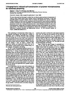
We have proven that our algorithm monotonically reduces the pattern metric, even for the case of reusable resources where we are unable to prove global convergence (since we are using an approximate algorithm to step through time). Unresolved, however, is the rate of convergence. In the introduction, we described a number of projects where we are using this methodology. We have consistently found that the Gauss-Seidel strategy produces very fast convergence. Figure 3 shows how well we match a historical pattern (normalized to 100) after each

28

110 108 Normalized metric

106 104 102 100 98 96 94 92 90 1

2

3

4

5

6

7

8

9

10

11

12

13

14

15

Iterations

Figure 3: Rate of convergence of the pattern metric. iteration of the algorithm. The model was judged to be “acceptable” (by a knowledgeable user) if the performance was within the bounds shown in the figure (approximately two percent above and below the target). We found that the Gauss-Seidel algorithm converged closely to this target within three to four iterations. We have used this algorithm in a number of projects, and this performance is typical. The fast performance is due to the ability of the algorithm to adjust after each time step whether it should do more or less of an activity in order to match a target statistic based on how well we are tracking the goal over the last T time periods (which may include time periods from a previous iteration). If we are using an approximate dynamic programming algorithm, we have to simulate the problem iteratively, and the pattern logic adds only a nominal computational burden. If we were to use a simple myopic policy which normally would require stepping through the data once, this logic now requires that we repeat this simulation three or four times.

6.2

Matching patterns and improving solution quality

We now report on experiments where we measure both how well the procedure matches exogenous patterns, and the degree to which patterns derived from solving a static model optimally improves the quality of heuristics used to solve the dynamic problem.

29

Data 20-200(1)-2000(1)-30 20-200(1)-4000(1)-60 20-200(1)-6000(1)-90 10-200(2)-4000(2)-60 40-200(3)-4000(3)-60

Linear Pattern Logic and a Myopic Policy % optimality % optimality % improvement with θ = 0 with θ = 10000 in obj. function 31.7 72.9 41.2 39.6 73.8 34.1 28.2 72.3 44.1 48.0 72.6 24.6 25.5 67.6 42.1

% improvement in pattern metric 81.6 73.5 82.9 83.3 73.3

Table 3: Effect of patterns when using a myopic policy (value functions are zero) and a linear pattern metric. Piecewise Linear Pattern Logic using a Myopic Policy % optimality % optimality % improvement % improvement with θ = 0 with θ = 10000 in obj. function in pattern metric 20-200(1)-2000(1)-30 31.7 76.3 44.6 71.0 20-200(1)-4000(1)-60 39.6 73.5 33.9 59.0 20-200(1)-6000(1)-90 28.2 69.6 41.5 81.6 10-200(2)-4000(2)-60 48.0 78.7 30.6 71.0 40-200(3)-4000(3)-60 25.5 68.8 43.3 70.7 Data

Table 4: Effect of patterns when using a myopic policy and a piecewise-linear pattern metric. Tables 3 and 4 summarize our experimental results when implementing our algorithm using a myopic policy. We see that there is a significant improvement in the percentage of optimality obtained by incorporating patterns using either the linear (equation (30)) or piecewise linear (equation (29)) versions of our algorithm. We are able to achieve in most cases around 70 percent of the optimal solution with an improvement of around 40 percent. While this is far below optimal, we have to point out that the myopic policy is especially poor. This policy does not allow us to move equipment empty to a different location to cover demands that might arise in the future, resulting in excess inventories of equipment at some location that become unproductive. We also see that in the implementations of both the linear and piecewise linear versions of our methodology there is a significant reduction in the pattern metric, showing that we are doing a much better job of matching the pattern. In tables 5 and 6 we report our results for incorporating patterns when we use linear value function approximations to convey information among subproblems. We see that even without incorporating patterns, with the use of linear value function approximations we are able to achieve more than 90 percent of the optimal solution. Despite this, both linear and

30

Linear Pattern Logic with Linear Value Function Approximation % optimality % optimality % improvement % improvement with θ = 0 with θ = 10000 in obj. function in pattern metric 20-200(1)-2000(1)-30 92.2 93.5 1.3 29.3 20-200(1)-4000(1)-60 91.4 92.7 1.3 32.0 20-200(1)-6000(1)-90 92.7 93.4 0.7 40.2 10-200(2)-4000(2)-60 94.0 95.5 1.4 35.1 40-200(3)-4000(3)-60 90.7 91.3 0.6 30.2 Data

Table 5: Effect of patterns when using a linear value function approximation and a linear pattern metric. Piecewise Linear Pattern Logic with Linear Value Function Approximation Data % optimality % optimality % improvement % improvement with θ = 0 with θ = 10000 in obj. function in pattern metric 20-200(1)-2000(1)-30 92.2 94.5 2.3 25.1 20-200(1)-4000(1)-60 91.4 94.1 2.7 29.6 20-200(1)-6000(1)-90 92.7 94.2 1.5 40.3 10-200(2)-4000(2)-60 94.0 97.4 3.3 31.2 40-200(3)-4000(3)-60 90.7 94.0 3.4 30.2

Table 6: Effect of patterns when using a linear value function approximation and a piecewiselinear pattern metric. piecewise linear pattern metrics improve overall solution quality, with the greatest benefits coming from the piecewise linear version. Since static patterns do not capture the temporal effect of moving resources it is reasonable to infer that our methodology is less effective as the number of time periods increases. This is validated in our experiments where the least improvement is observed for the dataset with the largest number of time periods (90). We also look at the behavior of our methodology as we change the scaling factor θ for a single data set “20-200(1)-2000(1)-30.” We show the percentage of optimality for the linear and piecewise linear versions of our algorithm using a myopic policy in figure 4. We see a monotonic increase in the percentage of optimality as θ increases. In figure 5 we plot the percentage of optimality for the experimental setup where we use linear value function approximations. We see that the best results occur over the range θ ∈ [500, 1000]. Using our methodology we are able to improve solution quality from 92.5 percent of the true optimum to almost 95 percent, a significant improvement given the overall quality of the solution. Note also that, in this particular case, that solution quality decreases if θ is too large. We believe this occurs because the solution quality using nonlinear value function 31

% Optimality

100 80 60 40 20 0 0

500

1000

2000

5000

10000

20000

Scaling factor No patterns

Piecewise Linear

Linear

Figure 4: Percentage optimality using a myopic policy.

% Optimality

100 95 90 85 80 0

500

1000

2000

5000

10000

20000

Scaling factor No patterns

Piecewise Linear

Linear

Figure 5: Percentage optimality with linear value function approximations. approximations is quite good, while errors in the static pattern (partly because it ignores timing, and partly because of our approximation for estimating the fraction of vehicles that are held in a location) eventually detract from the solution. Thus, if the solution to the dynamic problem is good enough, it will be necessary to calibrate the weighting factor θ to obtain the best results. We plot the pattern metric as a function of the scaling factor for our experiment in figures 6 and 7. We see that in all cases the pattern metric monotonically decreases as the scaling factor increases. Since the value of the pattern metric directly measures the deviation from the static flow patterns these results prove validation of our methodology in representing information pertaining to static flow patterns in a time-staged setting. By increasing the

32

Pattern Metric

50 40 30 20 10 0 0

500

1000

2000

5000

10000

20000

Scaling factor Piecewise Linear

Linear

Figure 6: Reduction in pattern metric using a myopic policy.

Pattern Metric

25 20 15 10 5 0 0

500

1000

2000

5000

10000

20000

Scaling factor Piecewise Linear

Linear

Figure 7: Reduction in pattern metric with linear value function approximations. scaling factor we are able to get closer to the static pattern flows.

7

Conclusions

This paper presents a new methodology to capture information from static flow patterns in time-staged resource allocation models. Static flow patterns can be used to represent spatial imbalances in demands that convey global information that is not accurately captured in a time-staged formulation. Our research presents a framework for using static flow patterns (in our case, derived by solving the static model optimally) which are then used to guide the flows in a much larger dynamic model.

33

We present two versions of the algorithm. The first uses a linear pattern matching term, while the second uses a piecewise linear pattern term. The piecewise linear version of our algorithm is motivated by a quadratic cost problem that guarantees a reduction of the pattern metric over the entire time horizon in the case of a resource allocation problem with nonreusable resources. We present experimental results in a multicommodity flow setting. We see that when using a myopic policy our algorithms show a reduction in the optimality gap for a wide range of values of the scaling factor applied to the pattern metric. In the situation where we use linear approximations for the value function the application of our algorithms yields a reduction in the optimality gap for smaller values of θ.

Acknowledgment This research was supported in part by grant AFOSR-FA9550-05-1-0121 from the Air Force Office of Scientific Research and NSF grant CMS-0324380.

Appendix Proof of theorem 1 Recall that x˜∗t is optimal to the subproblem at time t where we solve the optimization model without the pattern metric. Obviously x∗t is also a feasible solution to the same problem since the feasible region is the same. Thus we have XX a∈A d∈Da

ctad x˜∗tad ≤

XX

ctad x∗tad .

(37)

a∈A d∈Da

34

Analogously x˜∗t is feasible to the optimization model in (23) and hence because of the optimality of x∗t to this model we have ! X Z x∗tad   θ ¯ ∗ + 2(u − x˜∗ ) du ≤ ctad x∗tad + h tad tad R a a∈A d∈Da d∈Da 0 ! X Z x˜∗tad  X X  θ ¯ ∗ + 2(u − x˜∗ ) du . ctad x˜∗tad + h tad tad R a 0 a∈A d∈D d∈D

X

X

(38)

a

a

It follows that:  X X  θ Z x∗tad   ∗ ∗ ¯ + 2(u − x˜ ) du − h tad tad R a 0 a∈A d∈Da  X X  θ Z x˜∗tad   ∗ ∗ ¯ + 2(u − x˜ ) du h tad tad R a 0 a∈A d∈Da XX (ctad x˜∗tad − ctad x∗tad ) . ≤

(39)

a∈A d∈Da

Combining equation (37) with equation (39) we have  X X  θ Z x∗tad   ∗ ∗ ¯ + 2(u − x˜ ) du − h tad tad R a 0 a∈A d∈Da  X X  θ Z x˜∗tad   ¯h∗ + 2(u − x˜∗ ) du ≤ 0. tad tad Ra 0 a∈A d∈D

(40)

a

We define the following L+ = {(a, d) : x∗tad ≥ x˜∗tad , a ∈ A, d ∈ Da } t L− = {(a, d) : x∗tad < x˜∗tad , a ∈ A, d ∈ Da }. t Then we can rewrite equation (40) in the following form X (a,d)∈L+ t

X (a,d)∈L− t

θ Ra Z

θ Ra

Z

x∗tad

x ˜∗tad x ˜∗tad

x∗tad

 ∗  ¯ + 2(u − x˜∗ ) du − h tad tad

 ∗  ¯ + 2(u − x˜∗ ) du ≤ 0. h tad tad

35

(41)

¯ ∗ in equation (41) using the expression in (22) we get Substituting for h tad x∗tad

  (u − x˜∗tad ) ∗,− s du − 2θ (ρtad − ρad ) + Ra x ˜∗tad + (a,d)∈Lt  X Z x˜∗tad  ∗,− (u − x˜∗tad ) s (ρadt − ρad ) + du ≤ 0. Ra x∗tad − X Z

(a,d)∈Lt

Integrating this expression gives us # " 2 2 ∗ ∗ ∗ ∗ ∗ X (x ) − (˜ x ) − 2˜ x (x − x ˜ ) tad tad tad tad ∗ s ˜∗tad ) + tad − 2θ (ρ∗,− tad − ρad )(xtad − x 2R a (a,d)∈L+ "t # 2 2 ∗ ∗ ∗ ∗ ∗ X (˜ x ) − (xtad ) − 2˜ xtad (˜ xtad − xtad ) s ≤ 0. 2θ (ρ∗,− x∗tad − x∗tad ) + tad tad − ρad )(˜ 2Ra − (a,d)∈Lt

It follows that "

# 2 ∗ ∗ (x − x ˜ ) tad s ∗ 2θ (ρ∗,− ˜∗tad ) + tad − tad − ρad )(xtad − x 2R a + (a,d)∈Lt " # 2 ∗ ∗ X (˜ x − x ) tad s (ρ∗,− ≤ 0. 2θ x∗tad − x∗tad ) − tad tad − ρad )(˜ 2R a − X

(42)

(a,d)∈Lt

We next need to introduce the pattern after subproblem t has been solved, which is given by ρ∗,+ tad

=

 t  ∗ X x0 t ad

t0 =0

Ra

 ∗  T X x˜t0 ad + Ra 0

∀a ∈ A,

∀d ∈ Da ∀t ∈ {1, . . . , T }.

t =t+1

∗,+ ∗,− Note that ρ∗,− tad differs from ρtad in that ρtad is defined before the subproblem at t is solved ∗,+ ∗,− and ρtad is defined after the subproblem is solved. ρ∗,+ tad is derived from ρtad by simply

replacing x˜∗tad with the optimal solution to the subproblem at t pertaining to the pattern (a, d) indicated by x∗tad . Now we derive the difference between the pattern metrics evaluated before and after solving the subproblem at time t, that is we have ! ∗ Ht∗ − Ht−1 = θ

X a∈A

Ra

X

2

s (ρ∗,+ tad − ρad ) −

X a∈A

d∈Da

36

Ra

X d∈Da

2

∗,− (ρtad − ρsad )

.

(43)

− Using the definitions of the sets L+ t and Lt we have

ρ∗,+ tad ρ∗,+ tad

 x∗tad − x˜∗tad = + ∀(a, d) ∈ L+ t Ra  ∗  xtad − x˜∗tad = ρ∗,− − ∀(a, d) ∈ L− t . tad Ra ρ∗,− tad



Thus we can rewrite equation (43) as shown Ht∗

−

∗ Ht−1



X

= θ

Ra

ρ∗,− tad

(a,d)∈L+ t

x∗ − x˜∗tad + ( tad ) − ρsad Ra

2

2 x˜∗tad − x∗tad s +θ Ra ) − ρad −( R a (a,d)∈L− t X X 2 2 ∗,− ∗,− −θ Ra (ρtad − ρsad ) − θ Ra (ρtad − ρsad ) . 

X

∗,− ρtad

(a,d)∈L− t

(a,d)∈L+ t

It follows that "

∗ Ht∗ − Ht−1 =θ

(x∗tad

− x˜∗tad )2 Ra 2

#

2 ∗,− (ρtad − ρsad )(x∗tad − x˜∗tad ) + − Ra + (a,d)∈Lt " # X 2 ∗,− (x∗tad − x˜∗tad )2 s ∗ ∗ θ Ra (ρ − ρad )(xtad − x˜tad ) + . Ra tad Ra 2 − X

Ra

(a,d)∈Lt

Thus we have "

∗ Ht∗ − Ht−1

# 2 ∗ ∗ (x − x ˜ ) tad = 2θ − ρsad )(x∗tad − x˜∗tad ) + tad − 2R a + (a,d)∈Lt " # 2 ∗ ∗ X (x − x ˜ ) ∗,− tad 2θ (ρtad − ρsad )(x∗tad − x˜∗tad ) + tad . 2R a − X

(ρ∗,− tad

(a,d)∈Lt

This is exactly the condition indicated by equation (42) which is satisfied by the optimal solution to the subproblem denoted by the model in (23). Thus we can conclude that ∗ Ht∗ − Ht−1 ≤ 0.

37

Since this is true for any time t the statement (24) is satisfied and our methodology is successful in reducing the pattern metric over the entire time horizon, that is we have HT∗ − H0∗ ≤ 0.

Proof of theorem 2 We prove theorem 2 that states our methodology of solving the optimization model in a pattern metric is exactly identical to the block coordinate descent (BCD) method for any iteration n ≥ 1. We first integrate the expression for f n (x) given in equation (27) given by

f n (x) =

X

X

a∈A

d∈Da

!  θ X ¯ ∗,n−1 ctad xtad + htad xtad + (xtad )2 − 2x∗,n−1 . tad xtad Ra d∈D

(44)

a

The objective function using the BCD methodology given by equation (28) has constant terms that do not affect the optimization. We first eliminate the following constant term

C

n−1

=

XX

(

T X

ct0 ad x∗,n−1 t0 ad ),

t=n−b

a∈A d∈Da t0 =1,t0 6=t

n−1 cT T

from the optimization since it is a constant. Then, for t = n − b n−1 cT , we have after T expansion arg min f BCD,n (x) = arg min x∈X

x∈X

XX

ctad xtad

a∈A d∈Da

 P  !2 T ∗,n−1 X θ X 0 0 x + x tad t =1,t 6=t t0 ad (Ra )2  + (ρsad )2  + Ra d∈D Ra a∈A a    T s X θ X X ∗,n−1 2ρ − xt0 ad + xtad  . (Ra )2  ad  R R a a 0 0 a∈A d∈D t =1,t 6=t

a

38

Again removing constant terms that do not affect the optimization from the above equation and expanding the quadratic terms we see that arg min f BCD,n (x) = arg min x∈X

XX

x∈X

ctad xtad

a∈A d∈Da

+

X θ Ra a∈A

+

X θ Ra a∈A

 P  !   T ∗,n−1 2 2 X xtad  t0 =1,t0 6=t xt0 ad (Ra )2  + Ra Ra d∈Da " # PT ∗,n−1 s X 0 0 2x ( x ) 0 2ρ tad t =1,t 6=t t ad − ad xtad . (Ra )2 2 Ra (Ra ) d∈Da

Removing constant terms again it follows that arg min f BCD,n (x) = arg min x∈X

XX

x∈X

ctad xtad

a∈A d∈Da

  T X θ X X s (xtad )2 + 2xtad (  x∗,n−1 + t0 ad ) − 2ρad Ra xtad . R a 0 0 a∈A d∈D t =1t 6=t

a

Adding and subtracting the term 2xtad x∗,n−1 in the above equation we get tad arg min f BCD,n (x) = arg min x∈X

x∈X

XX

ctad xtad

a∈A d∈Da

" # T X X θ X 2 ∗,n−1 ∗,n−1 (xtad ) + 2xtad ( xt0 ad ) − 2xtad xtad − 2ρsad Ra xtad . + R a a∈A d∈D t0 =0 a

It follows that arg min f BCD,n (x) = arg min x∈X

x∈X

XX

ctad xtad

a∈A d∈Da





 X θ X (xtad )2 + xtad ∗ 2Ra + Ra d∈D   a∈A a |

39

!  P  ( Tt0 =0 x∗,n−1 ) 0 ∗,n−1  s t ad − ρad −2xtad xtad  . Ra  {z } I

¯ ∗,n−1 . Substituting using this expression Term I is simply the gradient of the pattern metric h tad and comparing with equation (44) we get arg min f BCD,n (x) = arg min x∈X

x∈X

XX

ctad xtad

a∈A d∈Da

X θ X  ¯ ∗,n−1 xtad − 2xtad x∗,n−1 + (xtad )2 + h tad tad Ra d∈D a∈A a

n

= arg min f (x) x∈X

which is the statement in the theorem given in equation (44). We next show that the function f BCD,n given by  f BCD,n (x) =

XX

(

a∈A d∈Da

+θ

X a∈A

Ra



T X

 ct0 ad x∗,n−1 t0 ad ) + ctad xtad

t0 =1,t0 6=t

X

PT

t0 =1,t0 6=t

d∈Da

x∗,n−1 t0 ad + xtad − ρsad Ra

!2 (45)

is strictly convex. A function f is strictly convex if for any λ ∈ (0, 1) we have and two vectors x and y in the feasible region X we have: f (λx + (1 − λ)y) < λf (x) + (1 − λ)f (y). It is easy to see that if f is linear or a constant we have f (λx + (1 − λ)y) = λf (x) + (1 − λ)f (y). Thus we propose to show strict convexity by ignoring the constant and linear terms of the expression of f BCD,n (x) given in (45). We also show strict convexity with respect to each variable xtad from which we can conclude f BCD,n (x) is strictly convex in the vector x. We define after removing the linear and constant terms of the function f BCD,n (x) and retaining the quadratic expression for each variable xtad :  ftad (x) = θRa

n ktad + xtad − ρhad Ra

2 , ∀t ∈ T 40

where n = ktad

T X t0 =1,t0 6=t

x∗,n−1 t0 ad ,

t=n−b

n−1 cT T

is a nonnegative constant. Expanding ftad and further removing constant and linear terms we see that the only quadratic term that remains is of the form kx2 where k is a positive number. We have: k(λx + (1 − λ)y)2 = kλ2 x2 + k(1 − λ)2 y 2 + 2kλ(1 − λ)xy Now: (λkx2 + (1 − λ)ky 2 ) − k(λx + (1 − λ)y)2 = kx2 (λ − λ2 ) + ky 2 ((1 − λ) − (1 − λ)2 ) −2kλ(1 − λ)xy = kλ(1 − λ)(x2 + y 2 − 2xy) = kλ(1 − λ)(x − y)2 > 0 This is exactly the condition for strict convexity.

References Ahuja, R., Magnanti, T. L. & Orlin, J. B. (1993), Network Flows, Prentice Hall, Englewood Cliffs, NJ. 17 Barnhart, C., Hane, C. & Vance, P. (2000), ‘Using branch-and-price-and-cut to solve origindestination integer multicommodity flow problems’, Operations Research 48(2), 318–326. 16 Bertsekas, D. & Tsitsiklis, J. (1996), Neuro-Dynamic Programming, Athena Scientific, Belmont, MA. 19 Bertsimas, D. & Patterson, S. (2000), ‘The traffic flow management rerouting problem in air traffic control: A dynamic network flow approach’, Transportation Science 34(3), 239–255. 17 Crainic, T. G., Gendreau, M. & Dejax, P. (1993), ‘Dynamic and stochastic models for the allocation of empty containers’, Operations Research 41, 102–126. 17 41

Godfrey, G. & Powell, W. B. (2002), ‘An adaptive, dynamic programming algorithm for stochastic resource allocation problems I: Single period travel times’, Transportation Science 36(1), 21–39. 19 Godfrey, G. A. & Powell, W. B. (2001), ‘An adaptive, distribution-free approximation for the newsvendor problem with censored demands, with applications to inventory and distribution problems’, Management Science 47(8), 1101–1112. 19 Hane, C. A., Barnhart, C., Johnson, E. L., Marsten, R. E., Nemhauser, G. L. & Sigismondi, G. (1995), ‘The fleet assignment problem: Solving a large scale integer program’, Mathematical Programming 70, 211–232. 16 Holmberg, K., Joborn, M. & Lundgren, J. T. (1998), ‘Improved empty freight car distribution’, Transportation Science 32, 163–173. 17 Jordan, W. & Turnquist, M. (1983), ‘A stochastic dynamic network model for railroad car distribution’, Transportation Science 17, 123–145. 17 Marar, A., Powell, W. B. & Kulkarni, S. (2006), ‘Capturing expert knowledge in resource allocation problems through low-dimensional patterns’, IIE Transactions 38(2), 159–172. 1 Minoux, M. (1984), ‘A polynomial algorithm for minimum quadratic cost flow problems’, European Journal of Operations Research 18, 377–387. 17 Minoux, M. (1986), ‘Solving integer minimum cost flows with separable convex cost objective polynomially’, Mathematical Programming Study 26, 237–239. 17 Ortega, J. & Rheinboldt, W. (1970), Iterative Solutions of Nonlinear Equations in Several Variables, Academic Press, New York, NY. 13 Pearson, K. (1900), ‘On the criterion that a given system of deviations from the probable in the case of a correlated system of variables is such that it can be reasonably supposed to have arisen from random sampling’, Philosophy Magazine 50, 157–172. 7 Powell, W. B. & Carvalho, T. A. (1997), ‘Dynamic control of multicommodity fleet management problems’, European Journal Of Operations Research 98, 522–541. 17 Powell, W. B. & Van Roy, B. (2004), Approximate dynamic programming for high dimensional resource allocation problems, in J. Si, A. G. Barto, W. B. Powell & D. W. II, eds, ‘Handbook of Learning and Approximate Dynamic Programming’, IEEE Press, New York. 3 Powell, W. B., Shapiro, J. A. & Sim˜ao, H. P. (2002), ‘An adaptive dynamic programming algorithm for the heterogeneous resource allocation problem’, Transportation Science 36(2), 231–249. 19 Powell, W., George, A., Bouzaiene-Ayari, B. & Simao, H. (2005), Approximate dynamic programming for high dimensional resource allocation problems, in ‘Proceedings of the IJCNN’, IEEE Press, New York. 3 Read, T. & Cressie, N. (1988), Goodness-of-fit statistics for discrete, multivariate data, Springer-Verlag, New York. 7 Rockafellar, R. T. (1972), Convex Analysis, second edn, Princeton University Press, Princeton, NJ. 14

42

Sargent, R. & Sebastian, D. (1973), ‘On the convergence of sequential minimization algorithms’, Journal of Optimization Theory and Applications 12, 565–575. 13 Si, J., Barto, A. G., Powell, W. B. & D. Wunsch II, e. (2004), Handbook of Learning and Approximate Dynamic Programming, IEEE Press, New York. 19 Strang, G. (1988), Linear Algebra, Harcourt Brace Jovanovich, Orlando, FL. 12 Topaloglu, H. & Powell, W. B. (2006), ‘Dynamic programming approximations for stochastic, time-staged integer multicommodity flow problems’, Informs Journal on Computing 18(1), 31–42. 2 Tseng, P. (2000), ‘Convergence of a block coordinate descent method for nondifferentiable minimization’, Journal of Optimization Theory and Applications 109(3), 475–493. 14 Warga, J. (1963), ‘Minimizing certain convex functions’, SIAM Journal of Applied Mathematics 11, 588–593. 13, 16

43