Feb 14, 2018 - adjusted accordingly to incorporate learning about the label noise. ..... We train using the Adam optimizer (Kingma & Ba, 2014) for 3 epochs with ..... seven layers, and train using gradient descent with Nesterov ... momentum.
Using Trusted Data to Train Deep Networks on Labels Corrupted by Severe Noise
Dan Hendrycks * 1 Mantas Mazeika * 1 Duncan Wilson 2 Kevin Gimpel 3
arXiv:1802.05300v1 [cs.LG] 14 Feb 2018
Abstract The growing importance of massive datasets with the advent of deep learning makes robustness to label noise a critical property for classifiers to have. Sources of label noise include automatic labeling for large datasets, non-expert labeling, and label corruption by data poisoning adversaries. In the latter case, corruptions may be arbitrarily bad, even so bad that a classifier predicts the wrong labels with high confidence. To protect against such sources of noise, we leverage the fact that a small set of clean labels is often easy to procure. We demonstrate that robustness to label noise up to severe strengths can be achieved by using a set of trusted data with clean labels, and propose a loss correction that utilizes trusted examples in a dataefficient manner to mitigate the effects of label noise on deep neural network classifiers. Across vision and natural language processing tasks, we experiment with various label noises at several strengths, and show that our method significantly outperforms existing methods.
1. Introduction Robustness to label noise is set to become an increasingly important property of supervised learning models. With the advent of deep learning, the need for more labeled data makes it inevitable that not all examples will have highquality labels. This is especially true of data sources that admit automatic label extraction, such as web crawling for images, and tasks for which high-quality labels are expensive to produce, such as semantic segmentation or parsing. Additionally, label corruption may arise in data poisoning (Li et al., 2016; Steinhardt et al., 2017). Both natural and malicious label corruption are known to sharply degrade the performance of classification systems (Zhu & Wu, 2004). We consider the scenario where we have access to a large set of examples with potentially corrupted labels and determine *
Equal contribution 1 University of Chicago 2 Foundational Research Institute 3 Toyota Technological Institute at Chicago. Correspondence to: Mantas Mazeika .
True
GLC (Ours)
1.0 0.8 0.6
Forward
Confusion Matrix 0.4 0.2 0.0
Figure 1: A label corruption matrix C (top left) and three matrix estimates for a corrupted CIFAR-10 dataset. Entry Cij is the probability that a label of class i is corrupted to class j, or Cij = p(˜ y = j|y = i). Our estimate matches the true corruption matrix closer than the confusion matrix and the Forward method. Further comparisons and method descriptions are in Section 4.3.
how much can be gained from access to a small set of examples where labels are considered gold standard. This scenario is realistic, as it is usually the case that a number of trusted examples have been gathered in the validation and test sets, and that more could be gathered if necessary. To leverage the additional information from trusted labels, we propose a new loss correction and empirically verify it on a number of vision and natural language datasets with label corruption. Specifically, we demonstrate recovery from extremely high levels of label noise, including the dire case when the untrusted data has a majority of its labels corrupted. Such severe corruption can occur in adversarial situations like data poisoning, or when the number of classes is large. In comparison to loss corrections that do not employ trusted data (Patrini et al., 2016), our method is significantly more
Using Trusted Data to Train Deep Networks
accurate in problem settings with moderate to severe label noise. Relative to a recent method which also uses trusted data (Li et al., 2017), our method is far more data-efficient and generally more accurate. These results demonstrate that systems can weather label corruption with access only to a small number of gold standard labels. The code is available at https://github.com/mmazeika/glc.
2. Related Work The performance of machine learning systems reliant on labeled data has been shown to degrade noticeably in the presence of label noise (Nettleton et al., 2010; Pechenizkiy et al., 2006). In the case of adversarial label noise, this degredation can be even worse (Reed et al., 2014). Accordingly, modeling, correcting, and learning with noisy labels has been well studied (Natarajan et al., 2013; Biggio et al., 2011; Frénay & Verleysen, 2014). The methods of (Mnih & Hinton, 2012), (Larsen et al., 1998), (Patrini et al., 2016) and (Sukhbaatar et al., 2014) allow for label noise robustness by modifying the model’s architecture or by implementing a loss correction. Unlike (Mnih & Hinton, 2012) who focus on binary classification of aerial images and (Larsen et al., 1998) who assume the labels are symmetric (i.e., that the noise and the labels are independent), (Patrini et al., 2016) and (Sukhbaatar et al., 2014) consider label noise in the multi-class problem setting with asymmetric labels. In (Sukhbaatar et al., 2014), the authors introduce a stochastic matrix measuring label corruption, note its inability to be calculated without access to the true labels, and propose a method of forward loss correction. Forward loss correction adds a linear layer to the end of the model and the loss is adjusted accordingly to incorporate learning about the label noise. In the work of (Patrini et al., 2016), they also make use of the forward loss correction mechanism, and propose an estimate of the label corruption estimation matrix which relies on strong assumptions and no clean labels. Contra (Sukhbaatar et al., 2014; Patrini et al., 2016), we make the assumption that during training the model has access to a small set of clean labels and use this to create our label noise correction. This assumption has been leveraged by others for the purpose of label noise robustness, most notably (Veit et al., 2017; Li et al., 2017; Xiao et al., 2015), and tenuously relates our work to the field of semi-supervised learning (Zhu, 2005; Chapelle et al., 2010). In (Veit et al., 2017), human-verified labels are used to train a label cleaning network by estimating the residuals between the noisy and clean labels in a multi-label classification setting. In the multi-class setting that we focus on in this work, (Li et al., 2017) propose distilling the predictions of a model trained on clean labels into a second network trained on the noisy
labels and the predictions of the first. Our work differs from these two in that we do not train neural networks on the clean labels alone.
3. Gold Loss Correction e of u examples (x, y˜), We are given an untrusted dataset D and we assume that these examples are potentially corrupted examples from the true data distribution p(x, y) with K classes. Corruption is according to a label noise distribution p(˜ y | y, x). We are also given a trusted dataset D of t examples drawn from p(x, y), where t/u � 1. We refer to t/u as the trusted fraction. Concretely, a web scraper labeling images from metadata may produce an untrusted set, while expert-annotated examples would form a trusted dataset and be a gold standard. In leveraging trusted data, we focus our investigation on the stochastic matrix correction approach used by (Sukhbaatar et al., 2014; Patrini et al., 2016). In this approach, a stochastic matrix is applied to the softmax output of a classifier, and the resulting new softmax output is trained to match the noisy labeling. If the stochastic matrix is engineered so as to approximate the label noising procedure, this approach can bring the original output close to the distribution of clean labels, under moderate assumptions. We explore two avenues of utilizing the trusted dataset to improve this approach. The first involves directly using the trusted data while training the final classifier. As this could be applied to existing stochastic matrix correction methods, we run ablation studies to demonstrate its effect. The second avenue involves using the additional information conferred by the clean labels to obtain a better matrix to use with the approach. As a first approximation, one could use a normalized confusion matrix of a classifier trained on the untrusted dataset and evaluated on the trusted dataset. We demonstrate, however, that this does not work as well as the estimate used by our method, which we now describe. Our method makes use of D to estimate the K × K matrix of corruption probabilities Cij = p(˜ y = j | y = i). Once this estimate is obtained, we use it to train a modified classifier from which we recover an estimate of the desired conditional distribution p(y | x). We call this method the Gold Loss Correction (GLC), so named because we make use of trusted or gold standard labels. 3.1. Estimating The Corruption Matrix To estimate the probabilities p(˜ y | y), we make use of the identity
p(˜ y | x) =
K X y=1
p(˜ y | y, x)p(y | x).
Using Trusted Data to Train Deep Networks
The left hand side of the equality can be approximated by e Let θ˜ be the parameters training a neural network on D. ˜ be its softmax output of this network, and let pˆ(˜ y | x; θ) vector. Given an example x and its true one-hot label y, the term on the right reduces to p(˜ y | y, x) = p(˜ y | x). In the case where y˜ is conditionally independent of x given y, this further reduces to p(˜ y | x) = p(˜ y | y). In the case where y˜ is not conditionally independent of x given y, we can still approximate p(˜ y | y). We know p(˜ y , y, x) p(x | y˜, y)p(˜ y | y)p(y) p(˜ y | y, x) = = p(y, x) p(x | y)p(y) p(x | y˜, y) = p(˜ y | y) . p(x | y) This forces p(˜ y | y, x)p(x | y) = p(˜ y | y)p(x | y˜, y). Integrating over all x gives us Z Z p(˜ y | y, x)p(x | y) dx = p(˜ y | y) p(x | y˜, y) dx = p(˜ y | y). We approximate the integral on the left with the expectation of p(˜ y | y, x) over the empirical distribution of x given y. More explicitly, let Ai be the subset of x in D with label i. b We have Denote our estimate of C by C. X bij = 1 C pˆ(˜ y = j | x) |Ai | x∈Ai 1 X = pˆ(˜ y = j | y = i, x) |Ai | x∈Ai
≈ p(˜ y = j | y = i). This is how we estimate our corruption matrix for GLC. The second equality comes from noting that if y is known, the preceding discussion implies p(˜ y | x) = p(˜ y | y, x). This approximation relies on pˆ(˜ y | x) being a good estimate of p(˜ y | x) and on the number of trusted examples of each class. 3.2. Training a Corrected Classifier b we follow the method of (Sukhbaatar et al., Now with C, 2014; Patrini et al., 2016) to train a corrected classifier. Given the K × 1 softmax output s of our classifier, we b We then reinitialize θ define the new outputs as s˜ := Cs. and train the model pˆ(˜ s | x; θ) on the noisy labels with crossentropy loss. If y˜ is conditionally independent of x given y, and if C is nonsingular, then � it follows from the �invertibility e = argminθ L s, D given that of C that argminθ L s˜, D b is a perfect estimate of C. C
We find using s˜ to work well in practice, even for some singular corruption matrices. We can further improve on this method by using the data in the trusted set to train the corrected classifier. On examples from the trusted set b to the encountered during training, we temporarily set C identity matrix to turn off the correction. This has the effect of allowing our label correction to handle a degree of instance-dependency in the label noise (Menon et al., 2016). A summary of our method is in the algorithm below. Algorithm G OLD L OSS C ORRECTION (GLC) 1: 2: 3: 4: 5: 6: 7: 8: 9: 10: 11: 12: 13: 14:
e loss ` Input: Trusted data D, untrusted data D, e with loss ` Train network f (x) = pˆ(e y |x; θ) on D b ∈ RK×K with zeros, K the number of classes Fill C for k = 1, . . . , K do num_examples = 0 for (xi , yi ) ∈ D such that yi = k do num_examples += 1 b k += f (xi ) {add f (xi ) to kth column} C end for b k /= num_examples C end for Initialize new model g(x) = pˆ(y|x; θ) e b Train g(x) with `(g(x), y) on D and `(Cg(x), ye) on D Output: Model pˆ(y|x; θ) •
•
4. Experiments We empirically demonstrate GLC on a variety of datasets and architectures under several types of label noise. 4.1. Description Generating Corrupted Labels. Suppose our dataset has t + u examples. We sample a set of t datapoints D, and the e which we probabilistically remaining u examples form D, corrupt according to a true corruption matrix C. Note that we do not have knowledge of which of our u untrusted examples are corrupted. We only know that they are potentially corrupted. e To generate the untrusted labels from the true labels in D, we first obtain a corruption matrix C. Then, for an example with true label i, we sample the corrupted label from the categorical distribution parameterized by the ith row of C. Comparing Loss Correction Methods. The GLC differs from previous loss corrections for label noise in that it reasonably assumes access to a high-quality annotation source. Therefore, to compare to other loss correction methods, we ask how each method performs when starting from the same dataset with the same label noise. In other words, the only additional information our method uses is knowledge of which examples are trusted, and which are potentially
Using Trusted Data to Train Deep Networks
0.4 0.2
1.0
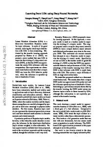
CIFAR-10, Uniform, 10% trusted
0.8
0.8
0.6
0.6
0.6
0.4
0.0 0.0 1.0
0.4 0.2
0.2 0.4 0.6 0.8 Corruption Strength
1.0
IMDB, Flip, 5% trusted
0.2
0.0 0.0 1.0
0.2 0.4 0.6 0.8 Corruption Strength
1.0
CIFAR-100, Hier., 10% trusted
0.0 0.0
0.6
0.6
0.6
0.6
0.2 0.0 0.0
0.2 0.2 0.4 0.6 0.8 Corruption Strength
1.0
0.0 0.0
Test Error
0.8
0.4
1.0
0.0 0.0
0.4 0.2
0.2 0.2 0.4 0.6 0.8 Corruption Strength
1.0
CIFAR-100, Uniform, 10% trusted
0.8
0.4
0.2 0.4 0.6 0.8 Corruption Strength
1.0
0.8
0.4
CIFAR-100, Flip, 10% trusted
0.4
0.8 Test Error
Test Error
1.0
0.2 0.4 0.6 0.8 Corruption Strength
1.0
0.8
0.2
0.0 0.0
SST, Flip, 1% trusted
1.0
Test Error
0.6
MNIST, Flip, 1% trusted
Test Error
Test Error
0.8
1.0
Test Error
GLC (Ours) Distillation Forward Gold Forward No Correction
Test Error
CIFAR-10, Flip, 10% trusted
1.0
0.2 0.4 0.6 0.8 Corruption Strength
1.0
0.0 0.0
0.2 0.4 0.6 0.8 Corruption Strength
1.0
Figure 2: Error curves for the compared methods across a range of corruption strengths on different datasets. corrupted. 4.2. Datasets, Architectures, and Noise Corrections MNIST. The MNIST dataset contains 28 × 28 grayscale images of the digits 0-9. The training set has 50,000 images and the test set has 10,000 images. For preprocessing, we rescale the pixels to a unit range. We train a 2-layer fully connected network each with dimension 256. The network is again optimized with Adam for 10 epochs, all while using batches of size 32 and a learning rate of 0.001. For regularization, we use `2 weight decay on all layers with λ = 1 × 10⁻⁶ . CIFAR. The two CIFAR datasets contain 32×32×3 color images. CIFAR-10 has ten classes, and CIFAR-100 has 100 classes. CIFAR-100 has 20 “superclasses” which partition its 100 classes into 20 semantically similar sets. We use these superclasses for hierarchical noise. Both datasets have 50,000 training images and 10,000 testing images. For both datasets, we train a Wide Residual Network (Zagoruyko & Komodakis, 2016) of depth 40. We train for 75 epochs using a widening factor of 2 and stochastic gradient descent with restarts (Loshchilov & Hutter, 2016). IMDB. The IMDB Large Movie Reviews dataset (Maas et al., 2011) contains 50,000 highly polarized movie reviews from the Internet Movie Database, split evenly into train and test sets. We pad and clip reviews to a length of 200 tokens, and learn 50-dimensional word vectors from scratch
for a vocab size of 5,000. We train an LSTM with 64 hidden dimensions on this data. We train using the Adam optimizer (Kingma & Ba, 2014) for 3 epochs with batch size 64 and the suggested learning rate of 0.001. For regularization, we use dropout (Srivastava et al., 2014) on the linear output layer with a keep probability of 0.8. Twitter. The Twitter Part of Speech dataset (Gimpel et al., 2011) contains 1,827 tweets annotated with 25 POS tags. The training set has 1,000 tweets, and the test set has 500. We use pretrained 50-dimensional word vectors, and for each token, we concatenate word vectors in a fixed window centered on the token. These form our training and test set. We use a window size of 3, and train a 1-layer fully connected network with hidden size 256, and use the nonlinearity from (Hendrycks & Gimpel, 2016). We train using the Adam optimizer for 15 epochs with batch size 64 and learning rate 0.001. For regularization, we use `2 weight decay with λ = 5 × 10⁻⁵ on all but the linear output layer. SST. The Stanford Sentiment Treebank dataset consists of single sentence movie reviews. There are 8,544 reviews in the training set and 2,210 in the test set. We use binarized labels for sentiment classification. Moreover, we pad and clip reviews to a length of 200 tokens and learn 100-dimensional word vectors from scratch for a vocab size of 10,000. Our classifier is a word-averaging model with an affine output layer. We use the Adam optimizer for 5 epochs with batch size 50 and learning rate 0.001. For regularization, we
CIFAR-100
CIFAR-10
MNIST
Using Trusted Data to Train Deep Networks
Corruption Type Uniform Uniform Uniform Flip Flip Flip Mean Uniform Uniform Uniform Flip Flip Flip Mean Uniform Uniform Uniform Flip Flip Flip Hierarchical Hierarchical Hierarchical Mean
Percent Trusted 5 10 25 5 10 25 5 10 25 5 10 25 5 10 25 5 10 25 5 10 25
Trusted Only 37.6 12.9 6.6 37.6 12.9 6.6 19.0 39.6 31.3 17.4 39.6 31.3 17.4 29.4 82.4 67.3 52.2 82.4 67.3 52.2 82.4 67.3 52.2 67.3
No Forward Correction Correction 12.9 14.5 12.3 13.9 9.3 11.8 50.1 51.7 51.1 48.8 47.7 50.2 30.6 31.8 31.9 9.1 31.9 8.6 32.7 7.7 53.3 38.6 53.2 36.5 52.7 37.6 42.6 23.0 48.8 47.7 48.4 47.2 45.4 43.6 62.1 61.6 61.9 61.0 59.6 57.5 50.9 51.0 51.9 50.5 54.3 47.0 53.7 51.9
Forward Gold 13.5 12.3 9.2 41.4 36.4 37.1 25.0 27.8 20.6 27.1 47.8 51.0 49.5 37.3 49.6 48.9 46.0 62.6 62.2 61.4 52.4 52.1 51.1 54.0
Distillation Confusion Correction Matrix 42.1 21.8 9.2 15.1 5.8 11.0 46.5 11.7 32.4 5.6 28.2 3.8 27.4 11.5 29.7 22.4 18.3 22.7 11.6 16.7 29.7 8.1 18.1 8.2 11.8 7.1 19.9 14.2 87.5 53.6 61.2 49.7 39.8 39.6 87.1 28.6 61.8 26.9 40.0 25.1 87.1 45.8 61.7 38.8 39.7 29.7 62.9 37.5
GLC (Ours) 10.3 6.3 4.7 3.4 2.9 2.6 5.0 9.0 6.9 6.4 6.6 6.2 6.1 6.9 42.4 33.9 27.3 27.1 25.8 24.7 34.8 30.2 25.4 30.2
Table 1: Vision dataset results. Percent trusted is the trusted fraction multiplied by 100. Unless otherwise indicated, all values are percentages representing the area under the error curve computed at 11 test points. The best mean result is shown in bold. use `2 weight decay with λ = 1 × 10⁻⁴ on the output layer. Forward Loss Correction. The forward correction b by trainmethod from (Patrini et al., 2016) also obtains C ing a classifier on the noisy labels, and using the resulting softmax probabilities. However, this method does not make use of a trusted fraction of the training data. Instead, it uses the argmax at the 97th percentile of softmax probabilities for a given class as a heuristic for detecting an example that is truly a member of said class. As in the original paper, we replace this with the argmax over all softmax probabilities for a given class on CIFAR-100 experiments. The estimate b is then used to train a corrected classifier in the same way C as GLC. Forward Gold. To examine the effect of training on trusted labels as done by GLC, we augment the Forward b estimate with the identity on method by replacing its C trusted examples. We refer to the resulting method as Forward Gold, which can be seen as an intermediate method between Forward and GLC. Distillation. The distillation method of (Li et al., 2017) involves training a neural network on a large trusted dataset
and using this network to provide soft targets for the untrusted data. In this way, labels are “distilled” from a neural network. If the classifier’s decisions for untrusted inputs are less reliable than the original noisy labels, then the network’s utility is limited. Thus, to obtain a reliable neural network, a large trusted dataset is necessary. A new classifier is trained using labels that are a convex combination of the soft targets and the original untrusted labels. 4.3. Uniform, Flip, and Hierarchical Corruption Corruption-Generating Matrices. We consider three types of corruption matrices: corrupting uniformly to all classes, i.e. Cij = 1/K, flipping a label to a different class, and corrupting uniformly to classes which are semantically similar. In order to create a uniform corruption at different strengths, we take a convex combination of an identity matrix and the matrix 11T /K. We refer to the coefficient of 11T /K as the corruption strength for a “uniform” corruption. A “flip” corruption at strength m involves, for each row, giving an off-diagonal column probability mass m and the entries along the diagonal probability mass 1 − m. Fi-
Twitter
IMDB
SST
Using Trusted Data to Train Deep Networks
Corruption Type Uniform Uniform Uniform Flip Flip Flip Mean Uniform Uniform Uniform Flip Flip Flip Mean Uniform Uniform Uniform Flip Flip Flip Mean
Percent Trusted 5 10 25 5 10 25 5 10 25 5 10 25 5 10 25 5 10 25
Trusted Only 45.4 35.2 26.1 45.4 35.2 26.1 35.6 36.9 26.2 22.2 36.9 26.2 22.2 28.5 35.9 23.6 16.3 35.9 23.6 16.3 25.3
No Correction 27.5 27.2 26.5 50.2 49.9 48.7 38.3 26.7 25.8 21.4 49.2 47.8 39.4 35.0 37.1 33.5 25.5 56.2 53.8 43.0 41.5
Forward 26.5 26.2 25.3 50.3 50.1 49.0 37.9 27.9 27.2 23.0 49.2 48.3 39.6 35.9 51.7 49.5 40.6 61.6 59.0 52.5 52.5
Forward Gold 26.6 25.9 24.6 50.3 49.9 47.3 37.4 27.6 26.1 20.1 49.2 47.5 36.6 34.5 44.1 40.2 26.4 54.8 48.9 36.7 41.9
Distillation Confusion Matrix 43.4 26.1 33.3 25.0 25.0 22.4 48.8 26.0 42.1 24.6 31.8 22.4 37.4 24.4 35.5 25.4 24.9 23.3 21.0 18.9 41.8 25.8 28.0 22.1 23.5 19.2 29.1 22.5 32.0 41.5 22.2 33.6 16.6 20.0 36.4 23.4 26.1 15.9 20.5 13.3 25.7 24.6
GLC (Ours) 24.2 23.5 21.7 24.9 23.5 21.7 23.3 25.0 22.3 18.7 25.2 22.0 18.5 22.0 31.0 22.3 15.5 15.8 12.9 12.8 18.4
Table 2: NLP dataset results. Percent trusted is the trusted fraction multiplied by 100. Unless otherwise indicated, all values are percentages representing the area under the error curve computed at 11 test points. The best mean result is bolded. nally, a more realistic corruption is hierarchical corruption. For this corruption, we apply uniform corruption only to semantically similar classes; for example, “bed” may be corrupted to “couch” but not “beaver” in CIFAR-100. For CIFAR-100, examples are deemed semantically similar if they share the same “superclass” or coarse label specified by the dataset creators. Experiments and Analysis of Results. We train the models described in Section 4.2 under uniform, label-flipping, and hierarchical label corruptions at various fractions of trusted data in the dataset. To assess the performance of GLC, we compare it to other loss correction methods and two baselines: one where we train a network only on trusted data without any label corrections, and one where the network trains on all data without any label corrections. Additionally, we report results on a variant of GLC that uses normalized confusion matrices, which we elaborate on in the discussion. We record errors on the test sets at the corruption strengths {0, 0.1, . . . , 1.0}. Since we compute the model’s accuracy at numerous corruption strengths, CIFAR experiments involves training over 500 Wide Residual Networks. In Tables 4 and 5, we report the area under the error curves across corruption strengths {0, 0.1, . . . , 1.0} for all baselines and corrections. A sample of error curves are displayed in Figure 2.
Across all experiments, GLC obtains better area under the error curve than the Forward and Distillation methods. The rankings of the other methods and baselines are mixed. On MNIST, training on the trusted data alone outperforms all methods save for GLC and Confusion Matrix, but performs significantly worse on CIFAR-100, even with large trusted fractions. Interestingly, Forward Gold performs worse than Forward on several datasets. We did not observe the same behavior when turning off the corresponding component of GLC, and believe it may be due to variance introduced during training by the difference in signal provided by the Forward method’s C estimate and the clean labels. The GLC provides a superior C estimate, and thus may be better able to leverage training on the clean labels. Additional results on SVHN, are in the supplementary materials. 4.4. Weak Classifier Labels Our next benchmark for GLC is to use noisy labels obtained from a weak classifier. This models the scenario of label noise arising from a classification system weaker than one’s own, but with access to information about the true labels that one wishes to transfer to one’s own system. For example, scraping image labels from surrounding text on web pages provides a valuable signal, but these labels would train a sub-par classifier without correcting the label noise.
Using Trusted Data to Train Deep Networks
Percent Trusted 1 CIFAR-10 5 10 Mean 5 CIFAR-100 10 25 Mean
Trusted Only 62.9 39.6 31.3 44.6 82.4 67.3 52.2 67.3
No Correction 28.3 27.1 25.9 27.1 71.1 66 56.9 64.7
Forward 28.1 26.6 25.1 26.6 73.9 68.2 56.9 66.3
Forward Gold 30.9 25.5 22.9 26.4 73.6 66.1 51.4 63.7
Distillation 60.4 28.1 17.8 35.44 88.3 62.5 39.7 63.5
Confusion Matrix 31.9 27 24.2 27.7 74.1 63.8 50.8 62.9
GLC (Ours) 26.9 21.9 19.2 22.7 68.7 56.6 40.8 55.4
Table 3: Results when obtaining noisy labels by sampling from the softmax distribution of a weak classifier. Percent trusted is the trusted fraction multiplied by 100. Unless otherwise indicated, all values are the percent error attained under the indicated correction. The best average result for each dataset is shown in bold. Weak Classifier Label Generation. To obtain the labels, we train 40-layer Wide Residual Networks on CIFAR-10 and CIFAR-100 with clean labels for ten epochs each. Then, we sample from their softmax distributions with a temperature of 5, and fix the resulting labels. This results in noisy labels which we use in place of the labels obtained through the uniform, flip, and hierarchical corruption methods. The weak classifiers obtain accuracies of 40% on CIFAR-10 and 7% on CIFAR-100. Despite the presence of highly corrupted labels, we are able to significantly recover performance with the use of a trusted set. Note that unlike the previous corruption methods, weak classifier labels have only one corruption strength. Thus, performance is measured in percent error rather than area under the error curve. Results are displayed in Table 6. Analysis of Results. Overall, GLC outperforms all other methods in the weak classifier label experiments. The Distillation method performs better than GLC by a small margin at the highest trusted fraction, but performs worse at lower trusted fractions, indicating that GLC enjoys superior data efficiency. This is highlighted by GLC attaining a 26.94% error rate on CIFAR-10 with a trusted fraction of 1%, down from the original error rate of 60%. It should be noted, however, that training with no correction attains 28.32% error on this experiment, suggesting that the weak classifier labels have low bias. The improvement conferred by GLC is more significant at higher trusted fractions.
5. Discussion and Future Directions Confusion Matrices. An intuitively reasonable alternative to GLC is to estimate C by a confusion matrix. To do this, one would train a classifier on the untrusted examples, obtain its confusion matrix on the trusted examples, rownormalize the matrix, and then train a corrected classifier as in GLC. However, GLC is a far more data-efficient and lower-variance method of estimating C. In particular, for
K classes, a confusion matrix requires at least K 2 trusted examples to estimate all entries of C, whereas GLC requires only K trusted examples. Another problem with using confusion matrices is that normalized confusion matrices give a biased estimate of C in the limit, due to using an argmax over class scores rather than randomly sampling a class. This leads to vastly overestimating the value in the dominant entry of each row, as can be seen in Figure 1. Correspondingly, we found GLC outperforms confusion matrices by a significant margin across nearly all experiments, with a smaller gap in performance on datasets where K, the number of classes, is smaller. Results are displayed in the main tables. We also found that smoothing the normalized confusion matrices was necessary to stabilize training on CIFAR-100. Data Efficiency. We have seen that GLC works for small trusted fractions, and we further corroborate its data efficiency by turning to the Clothing1M dataset (Xiao et al., 2015). Clothing1M is a massive dataset with both humanannotated and noisy labels, which we use to compare the data efficiency of GLC to that of Distillation when very few trusted labels are present. The Clothing1M dataset consists of 1 million noisily labeled clothing images obtained by crawling online marketplaces. 50,000 images have humanannotated examples, from which we take subsamples as our trusted set. For both GLC and Distillation, we first fine-tune a pretrained 34-layer ResNet on untrusted training examples for four epochs, and use this to estimate our corruption matrix. Thereafter, we fine-tune the network for four more epochs on the combined trusted and untrusted sets using the respective method. During fine tuning, we freeze the first seven layers, and train using gradient descent with Nesterov momentum and a cosine learning rate schedule. For preprocessing, we randomly crop to a resolution of 224 × 224, and use mirroring. We also upsample the trusted dataset, finding this to give better performance for both methods.
Percent Accuracy
Using Trusted Data to Train Deep Networks
70
Distillation GLC (Ours)
60 50 40 30
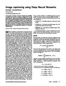
100 500 1000 Number of Trusted Examples
Figure 3: Data efficiency of our method compared to Distillation on Clothing1M.
As shown in Figure 3, GLC outperforms Distillation by a large margin, especially at lower numbers of trusted examples. This is because Distillation requires fine-tuning a classifier on the trusted data alone, which generalizes poorly with very few examples. By contrast, estimating the C matrix can be done with very few examples. Correspondingly, we find that our advantage decreases as the number of trusted examples increases. With more trusted labels, performance on Clothing1M saturates as evident in Figure 3. We consider the extreme and train on the entire trusted set for Clothing1M. We fine-tune a pre-trained 50-layer ResNeXt (Xie et al., 2016) on untrusted training examples to estimate our corruption matrix. Then, we fine-tune the ResNeXt on all training examples. During fine-tuning, we use gradient descent with Nesterov momentum. During the first two epochs, we tune only the output layer with a learning rate of 10−2 . Thereafter, we tune the whole network at a learning rate of 10−3 for two epochs, and for another two epochs at 10−4 . Then we apply our loss correction. Now, we fine-tune the entire network at a learning rate of 10−3 for two epochs, continue training at 10−4 , and early-stop based upon the validation set. In a previous work, (Xiao et al., 2015) obtain 78.24% in this setting. However, our method obtains a state-of-the-art accuracy of 80.67%, while with this procedure the Forward method only obtains 79.03% accuracy. b Estimation. For some datasets, the classifier Improving C pˆ(˜ y | x) may be a poor estimate of p(˜ y | x), presenting a b for GLC. To see the extent bottleneck in the estimation of C to which this could impact performance, and whether simple methods for improving pˆ(˜ y | x) could help, we ran several variants of GLC experiment on CIFAR-100 under the label flipping corruption at a trusted fraction of 5/100 which we now describe. For all variants, we averaged the area under
the error curve over five random initializations. b 1. In the first variant, we replaced GLC estimate of C with C, the true corruption matrix used for generating the noisy labels. 2. As demonstrated by (Guo et al., 2017), modern deep neural network classifiers tend to have overconfident softmax distributions. We found this to be the case with our pˆ(˜ y | x) estimate, despite the higher entropy of the noisy labels, and used the temperature scaling confidence calibration method proposed in the paper to calibrate pˆ(˜ y | x). 3. Suppose we know the base rates of corrupted labels ˜b, where ˜bi = p(˜ y = i), and the base rate of true labels b0 corrupted the b of the trusted set. If we posit that C Tb labels, then we should have b C0 = ˜bT . Thus, we may obtain a superior estimate of the corruption matrix b = argmin b kbT C b0 − by computing a new estimate C C ˜bT k + λkC b−C b0 k2 subject to C1 b = 1. 2 b We found that using the true corruption matrix as our C provides a benefit of 0.96 percentage points in area under the error curve, but neither the confidence calibration nor the base rate incorporation was able to change the performance from the original GLC. This indicates that GLC is robust to the use of uncalibrated networks for estimating C, and that improving its performance may be difficult without directly improving the performance of the neural network used to estimate pˆ(y | x). Better Performance for Worst-Case Corruption. The uniform corruption that we use in experiments is an example of worst-case corruption in the sense that the mutual information between y˜ and y is zero when the corruption strength equals 1.0. We found that training on the trusted dataset only resulted in superior performance at this corruption setting, especially on Twitter. This indicates that it may be possible to devise a re-weighting of the loss on trusted and untrusted examples using information theoretic b that would improve performance measures obtained from C in worst-case regimes.
6. Conclusion In this work we have shown the impact of having a small set of trusted examples on classifier label robustness. We proposed the Gold Loss Correction (GLC), a method for handling label noise. This method leverages the assumption that the model has access to a small set of correct labels to yield accurate estimates of the noise distribution. In our experiments, GLC surpasses previous label robustness methods across various natural language processing and vision domains which we showed by considering several
Using Trusted Data to Train Deep Networks
corruptions and numerous strengths. Consequently, GLC is a powerful, data-efficient label corruption correction.
References Biggio, B, Nelson, B, and Laskov, P. Support vector machines under adversarial label noise. ACML, 2011. Chapelle, Olivier, Schlkopf, Bernhard, and Zien, Alexander. Semi-Supervised Learning. The MIT Press, 1st edition, 2010. Frénay, Benoît and Verleysen, Michel. Classification in the presence of label noise: a survey. IEEE Trans Neural Netw Learn Syst, 25(5):845–869, May 2014. Gimpel, Kevin, Schneider, Nathan, O’Connor, Brendan, Das, Dipanjan, Mills, Daniel, Eisenstein, Jacob, Heilman, Michael, Yogatama, Dani, Flanigan, Jeffrey, and Smith, Noah A. Part-of-speech tagging for twitter: Annotation, features, and experiments. In Proceedings of the 49th Annual Meeting of the Association for Computational Linguistics: Human Language Technologies: Short Papers - Volume 2, HLT ’11, pp. 42–47, Stroudsburg, PA, USA, 2011. Association for Computational Linguistics. Guo, Chuan, Pleiss, Geoff, Sun, Yu, and Weinberger, Kilian Q. On calibration of modern neural networks. CoRR, abs/1706.04599, 2017. URL http://arxiv.org/ abs/1706.04599. Hendrycks, Dan and Gimpel, Kevin. Bridging nonlinearities and stochastic regularizers with gaussian error linear units. 27 June 2016. Kingma, Diederik P. and Ba, Jimmy. Adam: A method for stochastic optimization. CoRR, abs/1412.6980, 2014. URL http://arxiv.org/abs/1412.6980. Larsen, J, Nonboe, L, Hintz-Madsen, M, and Hansen, L K. Design of robust neural network classifiers. In Acoustics, Speech and Signal Processing, 1998. Proceedings of the 1998 IEEE International Conference on, volume 2, pp. 1205–1208 vol.2, May 1998. Li, Bo, Wang, Yining, Singh, Aarti, and Vorobeychik, Yevgeniy. Data poisoning attacks on factorization-based collaborative filtering. CoRR, abs/1608.08182, 2016. URL http://arxiv.org/abs/1608.08182. Li, Yuncheng, Yang, Jianchao, Song, Yale, Cao, Liangliang, Luo, Jiebo, and Li, Jia. Learning from noisy labels with distillation. CoRR, abs/1703.02391, 2017. URL http: //arxiv.org/abs/1703.02391. Loshchilov, Ilya and Hutter, Frank. SGDR: stochastic gradient descent with restarts. CoRR, abs/1608.03983, 2016. URL http://arxiv.org/abs/1608.03983.
Maas, Andrew L., Daly, Raymond E., Pham, Peter T., Huang, Dan, Ng, Andrew Y., and Potts, Christopher. Learning word vectors for sentiment analysis. In Proceedings of the 49th Annual Meeting of the Association for Computational Linguistics: Human Language Technologies, pp. 142–150, 2011. Menon, Aditya Krishna, van Rooyen, Brendan, and Natarajan, Nagarajan. Learning from binary labels with instancedependent corruption. CoRR, abs/1605.00751, 2016. URL http://arxiv.org/abs/1605.00751. Mnih, Volodymyr and Hinton, Geoffrey E. Learning to label aerial images from noisy data. In Proceedings of the 29th International Conference on Machine Learning (ICML-12), pp. 567–574, 2012. Natarajan, Nagarajan, Dhillon, Inderjit S, Ravikumar, Pradeep K, and Tewari, Ambuj. Learning with noisy labels. In Burges, C J C, Bottou, L, Welling, M, Ghahramani, Z, and Weinberger, K Q (eds.), Advances in Neural Information Processing Systems 26, pp. 1196–1204. Curran Associates, Inc., 2013. Nettleton, David F, Orriols-Puig, Albert, and Fornells, Albert. A study of the effect of different types of noise on the precision of supervised learning techniques. Artif Intell Rev, 33(4):275–306, 1 April 2010. Patrini, Giorgio, Rozza, Alessandro, Menon, Aditya, Nock, Richard, and Qu, Lizhen. Making deep neural networks robust to label noise: a loss correction approach. 13 September 2016. Pechenizkiy, M, Tsymbal, A, Puuronen, S, and Pechenizkiy, O. Class noise and supervised learning in medical domains: The effect of feature extraction. In 19th IEEE Symposium on Computer-Based Medical Systems (CBMS’06), pp. 708–713, 2006. Reed, Scott, Lee, Honglak, Anguelov, Dragomir, Szegedy, Christian, Erhan, Dumitru, and Rabinovich, Andrew. Training deep neural networks on noisy labels with bootstrapping. 20 December 2014. Srivastava, Nitish, Hinton, Geoffrey, Krizhevsky, Alex, Sutskever, Ilya, and Salakhutdinov, Ruslan. Dropout: A Simple Way to Prevent Neural Networks from Overfitting. Journal of Machine Learning Research, 15:1929–1958, 2014. Steinhardt, Jacob, Koh, Pang Wei, and Liang, Percy. Certified defenses for data poisoning attacks. In NIPS, 2017. Sukhbaatar, Sainbayar, Bruna, Joan, Paluri, Manohar, Bourdev, Lubomir, and Fergus, Rob. Training convolutional networks with noisy labels. 9 June 2014.
Using Trusted Data to Train Deep Networks
Veit, Andreas, Alldrin, Neil, Chechik, Gal, Krasin, Ivan, Gupta, Abhinav, and Belongie, Serge J. Learning from noisy large-scale datasets with minimal supervision. CoRR, abs/1701.01619, 2017. URL http://arxiv. org/abs/1701.01619. Xiao, Tong, Xia, Tian, Yang, Yi, Huang, Chang, and Wang, Xiaogang. Learning from massive noisy labeled data for image classification. In 2015 IEEE Conference on Computer Vision and Pattern Recognition (CVPR), pp. 2691–2699, June 2015. Xie, Saining, Girshick, Ross, Dollár, Piotr, Tu, Zhuowen, and He, Kaiming. Aggregated residual transformations for deep neural networks. arXiv preprint arXiv:1611.05431, 2016. Zagoruyko, Sergey and Komodakis, Nikos. Wide residual networks. 23 May 2016. Zhu, X. Semi-supervised learning literature survey. 2005. Zhu, Xingquan and Wu, Xindong. Class noise vs. attribute noise: A quantitative study. Artificial Intelligence Review, 22(3):177–210, 1 November 2004.
Using Trusted Data to Train Deep Networks
CIFAR-100
CIFAR-10
SVHN
MNIST
A. Additional Results and Figures Corruption Type Uniform Uniform Uniform Flip Flip Flip Mean Uniform Uniform Uniform Flip Flip Flip Mean Uniform Uniform Uniform Flip Flip Flip Mean Uniform Uniform Uniform Flip Flip Flip Hierarchical Hierarchical Hierarchical Mean
Percent Trusted 5 10 25 5 10 25 0.1 1 5 0.1 1 5 5 10 25 5 10 25 5 10 25 5 10 25 5 10 25
Trusted Only 37.56 12.93 6.62 37.56 12.93 6.62 19.04 80.42 79.66 24.28 80.42 79.66 24.28 61.45 39.6 31.26 17.43 39.6 31.26 17.43 29.43 82.37 67.28 52.21 82.37 67.28 52.21 82.37 67.28 52.21 67.29
No Forward Correction Correction 12.89 14.47 12.3 13.85 9.25 11.8 50.14 51.66 51.1 48.84 47.69 50.24 30.56 31.81 25.45 26.2 25.5 24.22 25.52 14.99 50.97 51.04 50.97 43.92 51.01 43.19 38.24 33.93 31.87 9.05 31.92 8.61 32.72 7.71 53.27 38.59 53.18 36.53 52.66 37.63 42.6 23.02 48.82 47.67 48.37 47.15 45.42 43.59 62.11 61.62 61.92 60.96 59.64 57.5 50.94 50.99 51.93 50.49 54.34 46.97 53.72 51.88
Forward Gold 13.5 12.3 9.2 41.41 36.37 37.14 24.99 26.76 24.92 15.65 50.93 49.46 49.02 36.12 27.85 20.59 27.1 47.78 51.02 49.47 37.3 49.59 48.88 45.98 62.62 62.19 61.41 52.36 52.07 51.13 54.02
Distillation Confusion Correction Matrix 42.08 21.81 9.21 15.09 5.78 11.01 46.55 11.65 32.37 5.63 28.21 3.77 27.37 11.49 80.93 25.71 80.39 28.23 24.06 2.67 89.11 19.81 86.27 17.81 17.56 2.22 63.05 16.07 29.73 22.42 18.34 22.69 11.62 16.65 29.66 8.13 18.1 8.16 11.77 7.06 19.87 14.18 87.48 53.64 61.2 49.7 39.82 39.61 87.11 28.58 61.85 26.93 39.96 25.14 87.12 45.75 61.71 38.84 39.73 29.7 62.89 37.54
GLC (Ours) 10.31 6.33 4.67 3.36 2.88 2.57 5.02 24.36 28.13 2.82 19.35 21.7 2.21 16.43 9.02 6.92 6.36 6.62 6.2 6.1 6.87 42.39 33.91 27.34 27.13 25.83 24.69 34.78 30.16 25.41 30.18
Table 4: Vision dataset results. Percent trusted is the trusted fraction multiplied by 100. Unless otherwise indicated, all values are percentages representing the area under the error curve computed at 11 test points. The best mean result is shown in bold.
Twitter
IMDB
SST
Using Trusted Data to Train Deep Networks
Corruption Type Uniform Uniform Uniform Flip Flip Flip Mean Uniform Uniform Uniform Flip Flip Flip Mean Uniform Uniform Uniform Flip Flip Flip Mean
Percent Trusted 5 10 25 5 10 25 5 10 25 5 10 25 5 10 25 5 10 25
Trusted Only 45.36 35.2 26.14 45.36 35.2 26.14 35.57 36.94 26.23 22.2 36.94 26.23 22.2 28.46 35.85 23.64 16.28 35.85 23.64 16.28 25.26
No Correction 27.48 27.21 26.53 50.19 49.9 48.69 38.33 26.68 25.76 21.44 49.16 47.8 39.42 35.04 37.1 33.45 25.51 56.23 53.83 42.99 41.52
Forward 26.55 26.19 25.33 50.33 50.08 48.99 37.91 27.94 27.19 23.0 49.2 48.26 39.57 35.86 51.68 49.52 40.6 61.59 59.01 52.49 52.48
Forward Gold 26.55 25.9 24.6 50.33 49.9 47.28 37.43 27.57 26.1 20.11 49.18 47.5 36.64 34.52 44.09 40.21 26.43 54.81 48.91 36.7 41.86
Distillation Confusion Matrix 43.37 26.11 33.34 25.03 24.96 22.39 48.77 26.01 42.11 24.58 31.84 22.39 37.4 24.42 35.47 25.45 24.89 23.33 21.01 18.93 41.84 25.8 28.03 22.1 23.48 19.2 29.12 22.47 32.01 41.48 22.22 33.62 16.59 20.04 36.44 23.38 26.15 15.93 20.53 13.25 25.66 24.62
GLC (Ours) 24.23 23.53 21.74 24.89 23.52 21.75 23.27 25.03 22.34 18.71 25.23 21.98 18.54 21.97 30.96 22.25 15.5 15.83 12.94 12.85 18.39
Table 5: NLP dataset results. Percent trusted is the trusted fraction multiplied by 100. Unless otherwise indicated, all values are percentages representing the area under the error curve computed at 11 test points. The best mean result is bolded.
Percent Trusted 1 CIFAR-10 5 10 Mean 5 CIFAR-100 10 25 Mean
Trusted Only 62.89 39.6 31.26 44.58 82.37 67.28 52.21 67.29
No Correction 28.32 27.12 25.9 27.11 71.07 66.01 56.87 64.65
Forward 28.07 26.6 25.13 26.6 73.92 68.23 56.86 66.34
Forward Gold 30.86 25.51 22.91 26.43 73.57 66.08 51.44 63.7
Distillation 60.42 28.12 17.79 35.44 88.29 62.51 39.69 63.50
Confusion Matrix 31.92 26.98 24.16 27.69 74.12 63.75 50.75 62.87
GLC (Ours) 26.94 21.89 19.15 22.66 68.69 56.65 40.82 55.39
Table 6: Results when obtaining noisy labels by sampling from the softmax distribution of a weak classifier. Percent trusted is the trusted fraction multiplied by 100. Unless otherwise indicated, all values are the percent error attained under the indicated correction. The best average result for each dataset is shown in bold.
Using Trusted Data to Train Deep Networks
0.4 0.2 0.0 0.0
0.2
0.4 0.6 0.8 Corruption Strength
1.0
CIFAR-100, Uniform, 10% trusted
0.2
0.4 0.6 0.8 Corruption Strength
CIFAR-100, Flip, 10% trusted
0.0 0.0
1.0
0.6
0.4 0.2
0.2
0.4 0.6 0.8 Corruption Strength
1.0
CIFAR-100, Uniform, 25% trusted Ours Distillation Forward Method Forward Gold Confusion All Data
0.4
0.0 0.0
1.0
0.2
0.4 0.6 0.8 Corruption Strength
1.0
CIFAR-100, Flip, 25% trusted
0.4 0.6 0.8 Corruption Strength 1.0
Test Error
Ours Distillation Forward Method Forward Gold Confusion All Data
0.4
1.0
1.0
0.6
0.6
0.4
0.2
0.4 0.6 0.8 Corruption Strength
CIFAR-10, Flip, 5% trusted
1.0
0.8
0.8
0.6
0.6
0.4
0.0 0.0
1.0
CIFAR-10, Uniform, 10% trusted
1.0
0.2
0.4 0.6 0.8 Corruption Strength
CIFAR-100, Hierarchical, 25% trusted
0.4
1.0
0.0 0.0
0.2
0.4 0.6 0.8 Corruption Strength
MNIST, Uniform, 0.1% trusted
1.0
Ours Distillation Forward Method Forward Gold Confusion All Data
0.4 0.6 0.8 Corruption Strength
0.4
0.0 0.0
1.0
CIFAR-10, Flip, 10% trusted
1.0
0.4 0.2
0.2
0.4 0.6 0.8 Corruption Strength
0.0 0.0
1.0
MNIST, Uniform, 1% trusted
1.0
0.6
0.6
0.6
0.6
0.8 0.6
0.4 0.6 0.8 Corruption Strength
1.0
CIFAR-10, Uniform, 25% trusted Ours Distillation Forward Method Forward Gold Confusion All Data
0.4
1.0
0.2 0.0 0.0
0.0 0.0
0.2 0.2
0.4 0.6 0.8 Corruption Strength
1.0
CIFAR-10, Flip, 25% trusted
0.4 0.6 0.8 Corruption Strength
1.0
0.0 0.0
1.0
0.8
0.8
0.6
0.6
0.4 0.2
0.2
0.4
0.0 0.0
0.2
0.4 0.6 0.8 Corruption Strength
1.0
MNIST, Uniform, 5% trusted Ours Distillation Forward Method Forward Gold Confusion All Data
0.4 0.6 0.8 Corruption Strength
1.0
0.4
0.0 0.0
0.4 0.6 0.8 Corruption Strength
1.0
MNIST, Flip, 1% trusted
0.4
0.0 0.0
1.0
0.2
0.4 0.6 0.8 Corruption Strength
1.0
MNIST, Flip, 5% trusted
0.8
0.2 0.2
0.2
0.2
Test Error
1.0
0.2
Test Error
0.0 0.0
0.2
Test Error
0.2
Test Error
0.8
Test Error
0.8
Test Error
0.8
0.4
MNIST, Flip, 0.1% trusted
0.6
0.8
0.4
1.0
0.8
0.2 0.2
1.0
0.2
0.2 0.4 0.6 0.8 Corruption Strength
1.0
CIFAR-100, Hierarchical, 10% trusted
0.0 0.0
0.8
0.0 0.0
0.4 0.6 0.8 Corruption Strength
0.4
0.8
Test Error
0.2
0.2
0.2
0.2
CIFAR-10, Uniform, 5% trusted
0.2
1.0
Test Error
0.4
Test Error
Test Error Test Error
0.2
0.6
0.2
Test Error
0.0 0.0
CIFAR-100, Hierarchical, 5% trusted
0.4
0.6
0.0 0.0
Test Error
0.4
0.6
0.2
1.0
0.6
0.8
0.8
0.0 0.0
0.6
0.8
1.0
0.6
0.8
0.8
0.0 0.0
0.8
0.8
1.0
0.2
1.0
1.0
0.2
Test Error
Test Error
1.0
CIFAR-100, Flip, 5% trusted
Test Error
1.0
Test Error
0.6
Ours Distillation Forward Method Forward Gold Confusion All Data
Test Error
Test Error
0.8
CIFAR-100, Uniform, 5% trusted
Test Error
1.0
0.6 0.4 0.2
0.2
0.4 0.6 0.8 Corruption Strength
1.0
0.0 0.0
0.2
0.4 0.6 0.8 Corruption Strength
1.0
Using Trusted Data to Train Deep Networks 1.0
0.0 0.0
1.0
0.4 0.6 0.8 Corruption Strength
SVHN, Uniform, 1% trusted
Ours Distillation Forward Method Forward Gold Confusion All Data
0.2
1.0
0.6
0.2
0.4 0.6 0.8 Corruption Strength
SVHN, Uniform, 5% trusted
0.4 0.6 0.8 Corruption Strength
0.2
0.4 0.6 0.8 Corruption Strength
0.0 0.0
1.0
SVHN, Flip, 1% trusted
1.0
Twitter, Uniform, 1% trusted
0.2 0.2
0.4 0.6 0.8 Corruption Strength
0.0 0.0
1.0
IMDB, Uniform, 5% trusted
1.0 0.8
0.6
0.6
0.6
0.4
0.6
Ours Distillation Forward Method Forward Gold Confusion All Data 0.2
0.4 0.6 0.8 Corruption Strength
0.0 0.0
SVHN, Flip, 5% trusted
1.0
Ours Distillation Forward Method Forward Gold Confusion All Data
0.4
1.0
0.4 0.2
1.0
0.4 0.6 0.8 Corruption Strength
Twitter, Flip, 1% trusted
0.2
0.4 0.6 0.8 Corruption Strength
0.0 0.0
1.0
IMDB, Uniform, 25% trusted
1.0 0.8
0.6
0.6
0.4
1.0
0.2
0.4 0.6 0.8 Corruption Strength
0.0 0.0
1.0
SST, Uniform, 0.1% trusted
1.0
0.6
0.6
0.6
1.0
0.2
0.4 0.6 0.8 Corruption Strength
0.0 0.0
1.0
Twitter, Uniform, 5% trusted
1.0
Test Error
0.6
Test Error
0.8
0.2
0.4 0.2
0.2
0.4 0.6 0.8 Corruption Strength
0.0 0.0
1.0
Twitter, Flip, 5% trusted
1.0
0.2
0.4 0.6 0.8 Corruption Strength
0.0 0.0
1.0
SST, Uniform, 1% trusted
1.0
0.6
0.6
0.6
0.6
0.0 0.0
1.0
0.2 0.2
0.4 0.6 0.8 Corruption Strength
1.0
Twitter, Uniform, 25% trusted
0.0 0.0
1.0
Test Error
0.8
Test Error
0.8
0.2
0.4 0.2
0.2
0.4 0.6 0.8 Corruption Strength
1.0
Twitter, Flip, 25% trusted
0.0 0.0
1.0
0.2
0.4 0.6 0.8 Corruption Strength
1.0
SST, Uniform, 5% trusted
0.0 0.0
1.0
0.6
0.6
0.6
0.0 0.0
0.2 0.2
0.4 0.6 0.8 Corruption Strength
1.0
0.0 0.0
Test Error
0.6
Test Error
0.8
Test Error
0.8
0.2
0.4 0.2
0.2
0.4 0.6 0.8 Corruption Strength
1.0
0.0 0.0
IMDB, Flip, 25% trusted
0.2
0.4 0.6 0.8 Corruption Strength
1.0
SST, Flip, 0.1% trusted
0.2
0.4 0.6 0.8 Corruption Strength
1.0
SST, Flip, 1% trusted
0.2
0.8
0.4
1.0
0.4
0.8
0.4
0.4 0.6 0.8 Corruption Strength
0.2
0.8
0.4
0.2
0.4
0.8
0.4
IMDB, Flip, 5% trusted
0.2
0.8
0.4
1.0
0.4
0.8
0.4
0.4 0.6 0.8 Corruption Strength
0.4
0.8
0.0 0.0
1.0
0.2
0.2
0.2 0.2
IMDB, Flip, 1% trusted
0.4
0.8
0.0 0.0
1.0
Test Error
0.2
0.2
Test Error
Test Error
0.2
0.4
0.8
0.0 0.0
Test Error
Ours Distillation Forward Method Forward Gold Confusion All Data
0.8
0.8
0.2
Test Error
0.4
1.0
Ours Distillation Forward Method Forward Gold Confusion All Data
0.2
1.0
0.6
0.0 0.0
1.0
0.4
0.0 0.0
0.6
Test Error
Test Error
0.8
0.6
0.2
Test Error
0.0 0.0
0.8
1.0
Test Error
Test Error
0.4
0.8
0.0 0.0
1.0
0.8 0.6
0.8
0.2 0.2
1.0
Test Error
0.2
IMDB, Uniform, 1% trusted
Test Error
0.4
1.0
Test Error
0.6
Ours Distillation Forward Method Forward Gold Confusion All Data
Test Error
Test Error
0.8
SVHN, Flip, 0% trusted
Test Error
SVHN, Uniform, 0% trusted
Test Error
1.0
0.2
0.4 0.6 0.8 Corruption Strength
1.0
SST, Flip, 5% trusted
0.4 0.2
0.2
0.4 0.6 0.8 Corruption Strength
1.0
0.0 0.0
0.2
0.4 0.6 0.8 Corruption Strength
1.0