different stations to a single satellite provides information about ionospheric behavior over ...... and Performance,. Ganga-Jamuna Press, Lincoln, Massachusetts.
Using WAAS Ionospheric Data to Estimate LAAS Short Baseline Gradients Seebany Datta-Barua, Todd Walter, Sam Pullen, Ming Luo, Juan Blanch, and Per Enge Stanford University
ABSTRACT The Local Area Augmentation System (LAAS) is intended to provide real-time differential GPS corrections with the high accuracy, availability, and integrity required for Category II/III landings. In order to meet these requirements, errors due to ionospheric effects must be bounded such that integrity is maintained with minimal loss of availability. This paper describes the process by which archived data provided by the Wide Area Augmentation System (WAAS) were used to determine the appropriate upper bound to sufficiently cover this error even during severe ionospheric storms. We seek an answer to the question of how much spatial variation in the ionospheric delay can be expected at distance scales comparable to those between the receivers at the LAAS ground facility (LGF) and an incoming aircraft. WAAS continuously processes ionospheric data, known as “supertruth”, for the Conterminous United States (CONUS) region, obtained from its triply-redundant network of twenty-five dual-frequency ground stations. Comparing the simultaneous zenith delays from two different stations to a single satellite provides information about ionospheric behavior over receiver separation distances only as short as the two nearest WAAS ground stations’ separation (i.e. 255 km). In order to gain an understanding of ionospheric error at LAAS-applicable distance scales, we compare the ionospheric delay of a single line-of-sight (LOS) at one epoch with the delay for the same LOS up to an hour later. We assume a quasistatic ionosphere over this time scale, and choose the ionospheric pierce point (IPP) separation as the distance most analogous to that between the LGF and the aircraft. Using data from days on which the ionosphere behaved nominally and days on which ionospheric storms
occurred, we observe the storm effects to exhibit significantly higher spatial gradients than the nominal periods. The bounds implied by these storms indicate that LAAS may need to revise its spatial ionospheric confidence bound to be broadcast. INTRODUCTION The ionosphere is a region of the upper atmosphere of the earth ionized primarily by solar ultraviolet radiation. Due to the free electrons in this region, electromagnetic signals traveling through the ionosphere, e.g. the GPS satellite broadcast, are delayed with respect to the same signal traveling through free space. The error introduced by the ionosphere into the GPS signal is highly variable and difficult to model. One of the functions of the Local Area Augmentation System (LAAS) is to provide differential GPS corrections to users within tens of kilometers of the LAAS Ground Facility (LGF). Moreover, LAAS must meet the demands in accuracy, availability, and integrity needed for Category II/III landings. For this reason, bounds must be placed on the difference in ionospheric errors between an incoming aircraft and the LGF with minimal loss in availability. To estimate these bounds, the LAAS configuration that must be modeled is that of the LGF and the aircraft separated by some distance on the order of kilometers viewing the same satellite and each suffering an ionospheric delay. In general these delay values will differ because the line-of-sight (LOS) of the LGF and the LOS of the aircraft each penetrate different parts of the ionosphere. In the limit as the LGF and the aircraft receivers’ separation approaches zero, the difference in ionospheric delay for the LOSs should vanish. In summary, we seek an estimate of the maximum spatial decorrelation at kilometer distances and to develop an
idea of the LAAS worst-case scenario that must be protected. In order to analyze the LAAS configuration, we must be able to measure the delay along two LOSs and a characteristic separation distance between the LOSs.
distance, each pair of stations chosen is spatially separated. Just as the LAAS concern is the simultaneous difference in the delays experienced by the LGF and the aircraft, with this method the delays for a single epoch are differenced.
Ionospheric data, known as “supertruth”, have been obtained for the past few years for the Conterminous United States (CONUS) region from the Wide Area Augmentation System (WAAS) network of twenty-five ground stations. Each ground station has triply-redundant dual-frequency receivers, allowing for a direct measurement of the ionospheric delay. The raw receiver data is first conditioned into “truth” by post-process carrier leveling and the removal of satellite and receiver biases. Then WAAS’s triple redundancy applies voting to remove receiver artifacts. The voting technique is to choose the median measurement at each epoch and define a tight bound on that value within which the other two receivers measurements must fall, or else the data for that epoch is not made available. Supertruth is the final result of the whole process.
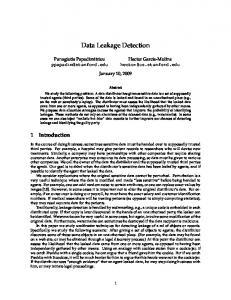
Figure 1 shows a two-dimensional histogram of the number of observations as a function of both the WAAS station separation distance and the difference in the slant ionospheric delay, dIs , for July 2, 2000, which exhibited nominal ionospheric behavior. This histogram was developed by counting the number of instances for which a particular separation distance yielded a particular difference in slant delay as the two stations tracked the same satellite. The horizontal axis divides station separation distances into bins, the vertical axis divides measurements of the difference in slant delay into bins, and the color of each pixel indicates the number of instances counted, on a logarithmic scale that spans more than 103 observations. To protect a user in all cases, the greatest difference in delay observed for each separation distance must be bounded.
The supertruth data include a measure of the total electron content (TEC) along each LOS, which is directly proportional to the delay in the signal. Although electron density as a function of height is generally a complicated function [Klobuchar 1996], the ionosphere can be approximated with the thin shell model, in which it is assumed that the entire ionosphere is a shell of finite thickness in which the TEC is contained. This shell is at an altitude of approximately 350 km, and the point of intersection of any LOS through this height is known as the “ionospheric pierce point” (IPP); it is the point at which the LOS has effectively penetrated the ionosphere. Supertruth allows us to use the TEC measurements associated with each of the IPPs scattered above the CONUS to map the spatial variation of the ionosphere over the U.S. at each epoch.
Although the “station pair” method has been used before [Klobuchar et al., 1993], it has certain limitations when applied to the LAAS scenario. First of all, the sampling over distance is discretized because the reference station locations are fixed. This results in segments of the x-axis (e.g. the 800 km region) for which there are no data. Also, there are no data for distances less than the smallest station separation (in this case, 255 km). In spite of these sampling issues, the fairly smooth behavior approaching the origin on the plot of nominal ionospheric data seems to imply that an upper envelope on the data may provide a bound, in units of meters per kilometer, on the spatial gradients at distances less than 255 km.
To find the maximum spatial decorrelation observed over kilometer distances, we use the supertruth data and focus on days known to have ionospheric disturbances. April 67, 2000, and July 15-16, 2000, were some of the most severely disturbed days for the current solar cycle. For comparison we analyze data from July 2, 2000, a day known to display nominal ionospheric behavior. STATION PAIR CONFIGURATION Our initial approach involved considering each pair of WAAS stations as the LGF -aircraft receiver pair. For each epoch the delays at each of two stations viewing the same satellite are differenced. This method is fairly intuitive, in that there is an exact analogue to each part of the LAAS configuration in this approach. In the same way that the LGF and the aircraft are separated by some
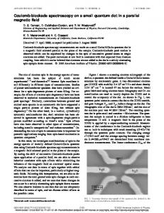
Figure 1: Nominal difference in slant ionospheric delay as a function of station separation distance. However, the two-dimensional histogram for April 6, on which there was an ionospheric disturbance, indicates otherwise (Figure 2). Spatial decorrelation does not occur
smoothly enough at distances greater than 255 km for a clean envelope of the plot to emerge. At 255 km, i.e. between New York and Boston, the slant delay is nearly 20 m. With the supertruth data available, the event of New York and Boston measuring a slant ionospheric delay difference of 20 m appeared to be due to the LOSs straddling a region of high TEC spatial gradient. However, without additional sampling at latitudes even further north, this could not be confirmed as a true event, and Boston and New York are two of the most northerly WAAS stations in that region of the continent.
single satellite to a single station at one epoch with the delay for the same LOS 10n seconds later (n = 1,2,3…) up to an hour later. In other words we measure the difference in the vertical ionospheric delay of a single LOS between time t = 0 and t = 10s, then between t = 0 and t = 20s, etc. Working with data from a single LOS eliminates receiver and satellite biases, but ionospheric dynamics can corrupt the results. We assume a quasistatic ionosphere over this time scale so that temporal decorrelation appro ximates spatial decorrelation. This method has a slightly different configuration from the actual LAAS LGF-aircraft scenario, so the connection it bears to the LAAS scenario may be less intuitive than the “station pair” method described above. In this situation only a single station’s measurements are under consideration, so the ability to equate one WAAS station to the LGF and a different WAAS station to the aircraft does not hold. Conceptually it is not exactly possible to equate a station at t=0 to, say, the LGF, and the same station at t = 10 s to the aircraft because that single reference station is fixed and effectively the separation distance is 0.
Figure 2: Difference in slant ionospheric delay as a function of station separation distance during an ionospheric storm. Figure 2, spatial gradient observation on a known storm day, emphasizes the severity of the sampling limitations of the station pair method. Information is available over receiver separation distances only as short as 255 km, and even the highest observed difference of 20 m at this distance could not be sufficiently confirmed by other measurements such that a decorrelation rate of 20/255 m/km could be established as the minimum upper bound. Also the envelope bounding the observations, when extrapolated down to zero separation, does not converge to zero difference. We know that physically the difference in delay must approach zero as the separation decreases, but it is difficult to determine an accurate model for distances less than 20 km based on this data. Ultimately this method of analysis was determined to be insufficient to provide a reliable decorrelation rate envelope at the 10 km distance separation. TIME STEP CONFIGURATION An alternate approach to bounding ionospheric decorrelation for LAAS was chosen to gain sufficient sampling at distances less than 255 km. With this configuration we compare the ionospheric delay from a
Although this approach bears less architectural resemblance to the LAAS scenario of interest, the reason that it achieves the same purpose as the station pair method is that over a time interval of seconds or even minutes, the elevation and azimuth angle of a single orbiting satellite at both times are similar. As a result, the LOSs slice through neighboring regions of the ionosphere. This achieves the same effect as an LGF receiver and an aircraft receiver whose LOSs to a given satellite penetrate neighboring areas of the ionosphere. In the LAAS configuration under study, the LGF and aircraft view a given satellite at similar elevation and azimuth angles. This method, therefore, allows for the comparison of similar regions of the ionosphere in measurements of difference in ionospheric delay, but since the reference station is fixed, the characteristic spatial separation distance between the two measurements must be redefined. The ionosphere, assumed in the thin shell model to be at an altitude of 350 km, is much closer to the LGF and aircraft than it is to the GPS satellite, which orbits at a height of about 20,000 km. For this reason, the IPPs associated with the LGF and the aircraft have a separation distance similar to the LGF-aircraft separation. In characterizing spatial decorrelation, then, IPP separation could be treated as the characteris tic length. In the “time step” method, there is only one receiver under consideration, but the IPP moves over time because the satellite is orbiting. In the time step approach the IPP separation is the characteristic distance taken as most analogous to that between the LGF and the aircraft.
In order to determine that the time step method overcomes the limitations that the station pair method has, we compare the two-dimensional histograms for April 6, 2000, as generated by each method of analysis. In order to compare the two methods we modify the station pair histogram from its form in Figure 2 to count observations as a function of zenith (rather than slant) delay and as a function, not of station separation distance, but of IPP separation. Furthermore, since the data analyzed via the station pair method in Figure 2 occurred every 100 seconds, for comparison we used the same data set with the time step method. As a result, the differences in delay could only be calculated 100n seconds apart via the time step method. Figures 3 and 4 compare the two dimensional histograms as a function of IPP separation and vertical ionospheric delay via the station pair method (3) and the time step method (4). The horizontal axis subdivides IPP separation distances into bins of width 40 km. The vertical axis separates the vertical ionospheric delay into .3 m wide bins. On both plots, the color indicates number of observations, but the scale is different for each plot. On Figure 3, dark red indicates 5000 observations, whereas for Figure 4 dark red indicates over 13,000 observations.
Figure 4: Difference in zenith ionospheric delay (in meters) as a function of IPP separation distance (km) during an ionospheric storm, as observed via the time step method.
With the time step method, the bounding envelope peaks at under 200 km with a highest observed vertical delay of nearly 17 meters. Even for separation distances between 0 and 40 km, there are differences in vertical delay as great as 9 m. These high gradients observed by the time step method conservatively bound the highest gradients (i.e. 10 m vertical delay at 250 km separation) observed by the station pair method. Calculating the decorrelation rate based on the Time Step approach should overbound the actual scenario. This method permits a more conservative estimate of the decorrelation rate than the station pair method.
Figure 3: Difference in zenith ionospheric delay (in meters) as a function of IPP separation distance (km) during an ionospheric storm, as observed via the station pair method. Overall the time step method achieves greater sampling. For IPP separation less than 100 km, in particular, the time step method yields extremely high sampling, compared with the complete lack of data in that range on Figure 3. Figure 4, a two dimensional histogram via the time step method, has high sampling at the kilometer range.
The fact that the envelope curve for Figure 4 decreases as the IPP separation increases beyond 200 km is most likely an effect of differencing measurements over time spans of up to only an hour. For a low elevation satellite an IPP to a station may cover a great distance in under an hour. In general, though, greater IPP separations may result from longer time intervals (i.e. greater than one hour) during which the satellite orbits. As a result, at greater IPP separation distances, sampling becomes less complete, though not nonexistent. In any case the time step method defines an envelope at IPP separation distances less than 100 km, which is the distance scale of interest for LAAS applications. Having checked the viability of the time step configuration as a method of analysis for the LAAS scenario, we produce a higher resolution two-dimensional histogram to see the finer structure to the bounding
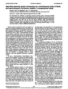
envelope at distances less than 100 km. For this analysis we difference over intervals of 10n up to an hour later and consider April 6, 2000, a day during which ionospheric disturbances are known to have occurred. Figure 5 is a two-dimensional histogram counting the number of events as a function of the IPP separation and the difference in the zenith ionospheric delay, dIv , on that day. The x-axis divides the IPP separation distance into kilometer-wide bins. The y-axis divides the measured dIv into segments of width 0.2 m. The color represents the number of observations on a logarithmic scale, with dark red indicating nearly 2 million observations. The data can be enveloped by a curve that converges to nearly zero at the origin, and whose steepest slope is the upper bound on the decorrelation rate. For LAAS threat model purposes, we are interested in the greatest dIv observed at a given IPP separation distance. Having examined the twodimensional histograms of each of several known ionospheric storm days in 2000 and 2001, including July 15-16, 2000, April 6 was determined to have had the steepest gradients.
VERIFICATION WITH RAW DATA To verify the observations made with the supertruth data via the time step method, namely, that at an IPP separation of 7 km the Washington, D.C., WAAS station (designated ZDC) measured a change in vertical delay to svn 40 of dIv =6m, we turned to the raw data from which supertruth is derived. In this way cycle slips or any smoothing and bias removal processes that might have yielded misleading results in our analysis would be visible. Figure 6 shows the slant ionospheric delay in meters at each of the three receivers at station ZDC (Washington, D.C.) as they track GPS satellite number 40 over time, measured in three ways at each receiver. The red line shows the ionospheric delay IL1ρ at the L1 frequency as measured by the L1-L2 code difference. The equation with which pseudorange measurements ρL1 and ρL2 at the L1 and L2 frequencies, respectively, can be used to measure the ionospheric delay IL1ρ at L1 is
I L1 ρ =
f L22 ( ρL 2 − ρL1 ) ( f L21 − f L22 )
(1)
where the L1 band frequency fL1 = 1575.42 MHz and L2 frequency fL2 =1227.60 MHz [Misra and Enge 2001]. This measurement of the slant ionospheric delay is the noisiest but unambiguous. The blue line plots the delay IL1φ at L1 as obtained from the L1 and L2 carrier phase measurements, φL1 and φL2 using the equation I L1φ =
2 f L2 2 2 ( f L1 − f L2 )
[ λL1 (φL1 − N L1 ) − λL 2 ( φL 2 − N L 2 )]
(2)
Figure 5: Difference in zenith ionospheric delay as a function of IPP separation during an ionospheric storm. The point on Figure 5 that defines the highest decorrelation rate observed occurs at 7 km, with an observed difference in vertical delay, dIv =6m. This was unexpectedly large and was investigated further. The highest gradient observed via the time step method occurred from the WAAS station at Washington, D.C., as it tracked svn 40 in the local mid-afternoon. Over a time span of two minutes the vertical ionospheric delay apparently dropped 6 m. With the supertruth data, however, an outage in ionospheric data for that station for tens of seconds made it unclear whether a cycle slip had occurred on any of the three receivers rendering the voting process unable to choose a median value to record.
where λL1 and λL2 are the wavelength of the L1 and L2 frequencies, respectively, and NL1 and NL2 are the unknown number of wavelengths in the carrier phase measurements at L1 and L2. The carrier measurement of the ionospheric delay is significantly less noisy than the code measurement. Due to the integer ambiguity of each carrier phase measurement, this measurement IL1φ of the delay was offset from the correct absolute value and was re-centered using the time-averaged code measurement IL1ρ . The green line is one-half the code-carrier divergence at L1, given by Equation 3:
I L1 ρφ =
ρL1 − φL1 2
(3)
The measurement of the ionospheric delay using only the L1 band also contained an ambiguity and was re-centered with the time -averaged code measurement of the delay, IL1ρ . The epochs that produced 6m vertical delay
Several features are apparent in Figure 5. First, it is clear there were no cycle slips for any of the receivers during the time interval in question. Second, all three receivers behave qualitatively identically. The curves for receiver 1 are offset by about 2 m with respect to the curves for receivers 2 and 3. This may have affected the voting process and contributed to the several second outage in the supertruth data. However, the identical timeevolution shown by all three receivers indicates that the observed anomaly was not due to receiver bias. At each receiver the three forms of delay measurement – code, carrier, and code-carrier divergence – drop by the same amount. At each receiver both the code measurement of the ionospheric slant delay (red) and code-carrier divergence (green) lag the carrier phase measurement (blue), the former to a significant extent. This behavior is an artifact of carrier smoothing of the code measurement, with a 5 s filter time constant for the L1 frequency and a 15 s time constant for the L2 frequency. These time constants correspond to the C-smooth values that were in effect for WAAS on April 6, 2000. Over a time interval of 110 s, the beginning and end of which are marked with vertical lines on Figure 6, the IPP tracked through a drop in the slant ionospheric delay of about 8 m, which corresponds to a zenith delay of 6 m, as was observed on Figure 5. The data appear to verify the observation from the supertruth data on Figure 5 that, on April 6, 2000, while station ZDC tracked svn 40, during a time span of 110s, corresponding to an IPP traversal of 7km, the IPP crossed an ionospheric front that caused a drop in zenith delay of 6m.
Receiver 1 iono delay (m) Receiver 2 iono delay (m)
20
Receiver 3 iono delay (m)
20
UTC 06/04/2000 21:32:12 - 21:34:02 44
20
43
18
42
16
41
14
40
12
39
10
Code msmt of delay at L1
38
8
L1 code-carrier divergence x 1/2 Carrier msmt of delay at L1
37
6
36
4
35
2
Slant Ionospheric Delay between Station ZDC and svn 40 20
The fact that the IPP crossed this front is illustrated by the map of the northeastern U.S. shown in Figure 7. The vertical and horizontal axes denote latitude and longitude, in degrees, with positive values north of the equator and east of the prime meridian. The WAAS stations in this region are marked with a star (*). Station ZDC is located at 39° N, 77.5° W. Superimposed on the outline of the U.S. is a color map that indicates the estimated vertical ionospheric delay at every location. The estimate is a linear interpolation between all IPP measurements in the supertruth data every 10 s spanning the times indicated with vertical lines in Figure 6. The IPPs from each station to svn 40 at UTC 21:32:12 and UTC 21:34:02 (the times marked with vertical lines in Figure 6) are shown with black circles, and a magenta line in the circle points to the station with which each IPP is associated. The IPPs associated with all other satellites are not illustrated; however, their locations are at the vertices of the triangles filled in by the interpolated color map. The two IPPs corresponding to the LOS between ZDC and svn40 appear nearly concentric on this map at 38° N, 79° W, though in actuality the later IPP is slightly NNE of the earlier IPP. The benefit of making a map of the ionosphere that has an “exposure time” of nearly two minutes is that the gradient observed at the IPPs between ZDC and svn 40 appears in sharp definition, separating the light green from the dark blue areas right near the pierce points. In addition it seems this gradient may be part of a larger structure, a front whose wall runs roughly east-west.
15 10 5 0 0
200
400
600
800
1000
1200
1400
1600
15
34 -82
10 5
Vertical Ionospheric Delay in m
difference at 7km IPP separation are marked with vertical lines. The horizontal axis below each plot marks the elapsed time in seconds.
0 -80 -78 -76 -74 -72 -70 Only ipps to svn 40 at 21:32:12 and 21:34:02 shown
0 0
200
400
600
800
1000
1200
1400
1600
0
200
400
600
800
1000
1200
1400
1600
15
Figure 7: Time -lapse map of IPP at 38°° N, 79°° W, crossing ionospheric storm front.
10 5 0
Elapsed time (s)
Figure 6: Slant ionospheric delay to svn 40 from each receiver at Washington, D.C., WAAS station.
We returned to Figure 5 to find an independent LOS to further confirm the ZDC-svn40 anomaly. In this case, we examined more closely the LOS that produced dIv = 8 m at an IPP separation of 15 km: station ZBW (Boston) to svn 24.
Receivers 1 and 3 at station ZBW both exhibit similar drops in the measured slant delay. At each receiver the drop in delay appears in all three forms of measurement: code (red), carrier (blue), and code-carrier divergence (green). The code measurement lags the carrier and codecarrier divergence delay measurements. This is, again, a byproduct of the carrier-aided smoothing process that takes place on each frequency’s pseudorange measurement ρ. From Figure 8 it appears that, while station ZBW tracked svn 24, during a span of 150s the slant ionospheric delay measured dropped 10 m. These values are consistent with the ones implied by the supertruth data analysis in Figure 5; 150 s corresponds to an IPP traversal of 15 km, and a 10 m slant delay corresponds to about 8 m zenith delay, given svn 24’s position in the sky during the time interval. Slant Ionospheric Delay between Station ZBW and svn 24
Figure 9 shows a map of the northeastern U.S. during the epochs that the LOS from ZBW to svn 24 exhibited a difference in zenith delay of 8 m over an IPP separation of 15 km. The axes indicate latitude and longitude in degrees, with positive values north and east. The WAAS stations in this region are marked with a star (*). Station ZBW, the Boston WAAS station, is located at about 43° N, 71.5° W. The IPPs from each station to svn 24 at UTC 20:00:22 and UTC 20:02:52 are shown as black circles, and a magenta line in the circle points to the station with which each is associated. These are the times corresponding to the vertical lines on the raw data in Figure 8. No other IPPs are explicitly shown, although they exist at the vertices where the shading changes color. A color map linearly interpolates vertical ionospheric delay between all empirical values of delay as recorded at IPPs every 10 s in the supertruth data. Ionospheric data spanning an interval of 2.5 minutes is used to produce a high definition illustration of the gradient that the IPP from ZBW to svn 24 exhibited. The IPPs between station ZBW and svn 24 at UTC 20:00:22 and UTC 20:02:52 are located at approximately 43°N and 76°W with the later IPP slightly to the northeast. Notice that again the IPPs mark a steep gradient that appears to be part of a larger front structure. UTC 06/04/2000 20:00:22 - 20:02:52 44
20
43
18
42
16
41
14
40
12
39
10
38
8
37
6
36
4
35
2
Receiver 1 iono delay (m)
30 Code msmt of delay at L1 L1 code-carrier divergence x 1/2 20
Vertical Ionospheric Delay in m
The raw data measurements of the ionosphere for this LOS over the time interval it exhibited its highest gradient in the supertruth data are shown in Figure 8. The raw data for receiver two at the Boston WAAS station were not available. The horizontal axis denotes elapsed time in seconds, and the vertical axis marks magnitude of the slant ionospheric delay in meters. The epochs whose difference produced the point identified on the histogram in Figure 5 for the LOS between ZBW and svn24 are marked with vertical lines. The red line is the dual frequency code measurement of the ionospheric delay IL1ρ at frequency L1, as given by Equation 1. The blue curve shows the dual frequency carrier phase measurement of the ionospheric delay IL1φ at L1 (Equation 2) and has been recentered to the mean of the code measurement IL1ρ to remove the integer ambiguity. The green curve illustrates the single-frequency code-carrier divergence measurement of the ionospheric error IL1ρ φ, as given by Equation 3 above.
Carrier msmt of delay at L1
10
34 -82 0 0
200
400
600
800
1000
1200
1400
1600
0 -80 -78 -76 -74 -72 -70 Only ipps to svn 24 at 20:00:22 and 20:02:52 shown
Figure 9: Time-lapse map of IPP crossing ionospheric storm front. ASSESSMENT OF ANOMALIES OBSERVED
Receiver 3 iono delay (m)
30
20
10
0 0
200
400
600
800
1000
1200
1400
Elapsed time (s)
Figure 8: Slant ionospheric delay to svn 24 from each receiver at Boston WAAS station (Data for receiver 2 not available).
1600
Supertruth data was used to identify two instances of particularly high gradients over IPP separation distances of several kilometers. In one case the anomaly in question was associated with the Washington, D.C., WAAS station and GPS satellite 40. In the other case an anomaly was associated with the Boston WAAS station and GPS satellite 24 an hour and a half earlier in the day.
The fact that two independent lines-of-sight exhibited high gradients seems to indicate that neither biases at an individual receiver or satellite nor anomalies occurring at either receiver or satellite contributed to the gradients. In each instance of anomalous behavior, the redundant receivers’ raw data measurements each corroborate the others. In each case the anomaly affected both the L1 and L2 frequencies, as evidenced by the code, carrier, and code-carrier divergence measurements of the ionospheric delay from the raw data. Because all alternate sources of error have been ruled out by this cross-verification, we conclude that the anomalous events that affected LOS ZDC-svn40 and LOS ZBW-svn24 were both records of actual ionospheric events. However, the gradients they imply (6m/7km and 8m/15 km vertical) may be artificially inflated for the following reason. Recall that in the maps of the eastern U.S. shown in Figures 7 and 9, the high gradients at particular IPPs seemed to be associated with a larger storm front structure. The anomaly at station ZBW as it tracked svn 24 preceded the anomaly along LOS ZDC-svn 40 by 1.5 hours. Examining maps similar to those in Figures 7 and 9 of epochs within this 1.5 hour time interval, we receive a rough indication that the storm front whose boundary runs roughly east-west recedes southward for the duration. Having first been traversed by an IPP from station ZBW, it progresses south to be traversed by an IPP from ZDC an hour and a half later. What this implies is that the storm front is moving at a rate comparable to the IPP velocities. With the time step method we assumed a quasi-static ionosphere so that temporal gradients were equivalent to spatial (IPP separation) gradients. If the same ionospheric storm front was near Boston on the afternoon of April 6, 2000, and then was near Washington, D.C. 1.5 hours later that day, then to first order its velocity was 110 m/s southward. Over this same time interval the IPPs associated with ZBW-svn24 and ZDC-svn40 were moving primarily northward with ground speeds of 7km/110s = 63 m/s and 15km/150s = 100 m/s, respectively. The velocity of the storm front is non-negligible compared to the IPP velocities. Since the velocities were directed roughly opposite to each other, the effect of the addition of the relative velocities would make the spatial gradient in the ionosphere appear to be a factor of two or more worse than it actually was. For example, recall that, for the LOS ZDC-svn40, over a span of 110s the IPP traversed 7 km, and the difference in vertical ionospheric delay was 6 m. During that 110s interval, assuming the front had a ground speed of 110 m/s, the storm front would have traveled 12 km. In the time that the IPP moved north 7 km, the ionospheric front moved south 12 km; this means that the purely spatial gradient of the ionosphere more likely 6 m vertical difference over a 19 km range than over 7 km. This analysis highlights the primary limitation of the time step
method of analyzing supertruth data: that spatial and temporal variation effects are mixed in together and it may not always be possible to decouple them. In the April 6 instance, an ionospheric front moved southward in a fairly visible manner, allowing for a rough calculation of its speed. The results of these estimates of the maximum spatial gradient observed using WAAS supertruth data are currently being used to build a ionospheric model for LAAS Integrity Monitoring Testbed (IMT) simulation. Preliminary tests indicate various IMT monitors can detect the anomaly in times ranging from 1.5 s to 30 s. Further simulation and verification remains to be done. The results described above also point toward a preliminary configuration of the LAAS worst-case scenario, one in which an ionospheric anomaly would affect the LOS of an incoming aircraft, but the LGF would be unaware of any such anomaly due to the sharp gradient. However, there are multiple relative motions that would need to be accounted for (the satellite, the aircraft, the IPP motion of the aircraft, the IPP motion of the LGF) in order to determine how long an aircraft could actually remain threatened before the IPP of the LGF started to pass through the gradient. Finally it is worth bearing in mind that such high spatial gradients only appeared on days known to have had particularly severe ionospheric storms as detected by WAAS. CONCLUSION After analyzing the WAAS supertruth data and using the raw data from which supertruth is derived for confirmation, we concluded that the phenomenon observed on April 6, 2000, seemed to be an actual ionospheric event, possibly associated with the auroral oval. Over a span of a couple of hours, a wall running east-west with a large north-south gradient moved southward. This occurrence is corroborated by colocated receivers exhibiting similar response, as well as noncolocated receivers. The observation is unlikely to be an artifact of codeless L2 tracking because L1-only processing was affected identically. This phenomenon was also seen during an ionospheric storm on July 15-16, 2000, but has not yet been fully analyzed. A more accurate estimate of the ionospheric front speed will help improve models for LAAS Integrity Monitoring simulations, as will connections of the event to broader ionospheric effects such as the auroral oval. Finally, it is worth bearing in mind that this is a worst case storm effect; on ionospherically quiet days there was no evidence of such large gradients. ACKNOWLEDGEMENTS We gratefully acknowledge the support of the FAA LAAS and WAAS Program Offices. We would also like
to thank Eric Altshuler at Raytheon for making the raw data available.
REFERENCES Christie, Jock R.I., Ping-Ya Ko, Boris Pervan, Per Enge, J. David Powell, and Brad Parkinson (1998). Analytical and Experimental Observations of Ionospheric and Tropospheric Decorrelation Effects for Differential Satellite Navigation during Precision Approach, Proc. ION GPS-98, pp. 739-748. Foster, John C. (2000). Quantitative Investigation of Ionospheric Density Gradients at Mid Latitudes, Proc. ION National Technical Meeting, pp. 447-453. Klobuchar, J. A., Patricia H. Doherty, and M. Bakry ElArini (1993). Potential Ionospheric Limitations to WideArea Differential GPS, Proc. ION GPS-93, Salt Lake City, UT, pp. 1245-1254. Klobuchar, J. A. (1996). Ionospheric Effects on GPS, in Global Positioning System: Theory and Application, Vol. I, B. Parkinson, J. Spilker, P. Axelrad, and P. Enge (Eds.), American Institute of Aeronautics and Astronautics, pp. 485-515. Misra, Pratap, and Per Enge (2001). Global Positioning System: Signals, Measurements, and Performance, Ganga-Jamuna Press, Lincoln, Massachusetts.