Using Wi-Fi Channel State Information (CSI) - UBC Open Collections

Using Wi-Fi Channel State Information (CSI) for Human Activity Recognition and Fall Detection by Tahmid Z. Chowdhury BEng (Hons), Electrical & Electronic Engineering, University of East London, 2014

A THESIS SUBMITTED IN PARTIAL FULFILLMENT OF THE REQUIREMENTS FOR THE DEGREE OF MASTER OF APPLIED SCIENCE in The Faculty of Graduate and Postdoctoral Studies (Electrical and Computer Engineering)

THE UNIVERSITY OF BRITISH COLUMBIA (Vancouver) April 2018 c Tahmid Z. Chowdhury, 2018

Abstract Human Activity Recognition (HAR) serves a diverse range of human-centric applications in health care, smart homes, and security. Recently, Wi-Fi-based solutions have attracted a lot of attention. The underlying principle of these is the effect that human bodies have on nearby wireless signals. The presence of static objects such as ceilings and furniture cause reflections while dynamic objects such as humans result in additional propagation paths. These effects can be empirically observed by monitoring the Channel State Information (CSI) between two Wi-Fi devices. As different human postures induce different signal propagation paths, they result in unique CSI signatures, which can be mapped to corresponding human activities. However, there are some limitations in current state-of-the-art solutions. First, the performance of CSI-based HARs degrade in complex environments. To overcome this limitation, we propose Wi-HACS: Leveraging Wi-Fi for Human Activity Classification using Orthogonal Frequency Division Multiplexing (OFDM) Subcarriers. In our work, we propose a novel signal segmentation method to accurately determine the start and end of a human activity. We use several signal pre-processing and noise attenuation techniques, not commonly used in CSI-based HAR, to improve the features obtained from the amplitude and phase signals. We also propose novel features based on subcarrier correlations and autospectra of principal components. Our results indicate that Wi-HACS can outperform the state-of-the-art method in both precision and recall by 8% in simple environments, and by 14.8% in complex environments. ii

Abstract The second limitation in existing CSI-HAR solutions is their poor performance in new/untrained environments. Since accurate Wi-Fi based fall detectors can greatly benefit the well-being of the elderly, we propose DeepFalls: Using Wi-Fi Spectrograms and Deep Convolutional Neural Nets for Fall Detection. We utilize the Hilbert Huang Transform spectrograms and train a Convolutional Neural Network to learn the features automatically. Our results show that DeepFalls can outperform the state-of-the-art RT-Fall in untrained environments with improvements in sensitivity and specificity by 11% and 15% respectively.

iii

Lay Summary Human Activity Recognition (HAR) serves a diverse range of human-centric applications in health care, smart homes, and security. Recently, Wi-Fi-based have attracted a lot of attention. When human beings are in the Wi-Fi range, the signals propagate differently. These effects can be empirically observed by measurements on the Wi-Fi channel. The channel variations can be used to classify different human activities. However, there are some limitations in existing Wi-Fi systems. First, the performances degrade in complex environments. To overcome this limitation, we propose Wi-HACS, which improves the state-of-the-art work’s precision and recall by 8% in simple environments, and by 15% in complex environments. The second limitation in existing systems is that they do not perform well in new environments. To improve the performances, we propose DeepFalls which make use of Convolutional Neural Network. Our results show that DeepFalls can outperform the state-ofthe-art method RT-Fall, in untrained environments with sensitivity and specificity improvements of 11% and 15% respectively.

iv

Preface This thesis is based on the research work performed under the supervision of Professor Cyril Leung. Chapter 2 is based on the conference paper titled “Wi-HACS: Leveraging WiFi for Human Activity Classification using OFDM Subcarriers’ correlation”, which was published in the 2017 5th IEEE Global Conference on Signal and Information Processing. This paper is co-authored by myself as the first author, Prof. Cyril Leung, and Prof. Chunyan Miao who is a Professor in the School of Computer Science and Engineering at Nanyang Technological University (NTU) in Singapore. I hereby confirm that I was the primary researcher of this work. I came up with the idea of the research independently. My contributions included conducting the literature review, collecting data, identifying the research problem and carrying out various signal processing and machine learning techniques under the supervision of Profs. Leung and Miao. Since there is no open dataset in this area, I used an open source firmware for an Intel 5300 Network Interface Card (NIC) to collect data. Prior to collecting data, an ethics approval was obtained from the UBC Behavioural Research Ethics Board for the project title: “DeepWi-Fi: Leveraging Channel State Information (CSI) of Wi-Fi and Deep Convolution Nets to Classify Human Gestures”, and the certificate number is H17-01839 .

v

Table of Contents Abstract

. . . . . . . . . . . . . . . . . . . . . . . . . . . . . . . . . . . . . . .

ii

Lay Summary . . . . . . . . . . . . . . . . . . . . . . . . . . . . . . . . . . . .

iv

Table of Contents . . . . . . . . . . . . . . . . . . . . . . . . . . . . . . . . . .

vi

List of Tables . . . . . . . . . . . . . . . . . . . . . . . . . . . . . . . . . . . . .

xi

List of Figures . . . . . . . . . . . . . . . . . . . . . . . . . . . . . . . . . . . .

xii

List of Abbreviations . . . . . . . . . . . . . . . . . . . . . . . . . . . . . . . . xviii Notation

. . . . . . . . . . . . . . . . . . . . . . . . . . . . . . . . . . . . . . .

xx

Acknowledgments . . . . . . . . . . . . . . . . . . . . . . . . . . . . . . . . . .

xxi

Dedication . . . . . . . . . . . . . . . . . . . . . . . . . . . . . . . . . . . . . . xxii 1

Introduction . . . . . . . . . . . . . . . . . . . . . . . . . . . . . . . . . . .

1

1.1

Sensors and Computer Vision based HAR . . . . . . . . . . . . . . . . .

1

1.2

Motivation behind the use of Wi-Fi

2

1.2.1

. . . . . . . . . . . . . . . . . . . .

Wi-Fi Channel and Human Activity Paradigm

. . . . . . . . . .

2

. . . . . . . . . . . . . . . . . . . . .

3

1.3

Related work on CSI based HAR

1.4

Technical Challenges in CSI-based HAR

. . . . . . . . . . . . . . . . .

5 vi

Table of Contents

2

1.5

Research Motivation and Contributions . . . . . . . . . . . . . . . . . .

6

1.6

Thesis organization . . . . . . . . . . . . . . . . . . . . . . . . . . . . .

9

Wi-HACS: A Wi-Fi based Human Activity Classification using OFDM Subcarriers . . . . . . . . . . . . . . . . . . . . . . . . . . . . . . . . . . . . . .

11

2.1

12

Channel State Information (CSI) . . . . . . . . . . . . . . . . . . . . . . 2.1.1

Correlation between human activities and amplitudes of OFDM Subcarriers . . . . . . . . . . . . . . . . . . . . . . . . . . . . .

2.1.2

2.3

Correlation between human activities and phases of OFDM Subcarriers . . . . . . . . . . . . . . . . . . . . . . . . . . . . . . .

16

OFDM Phase Calibration

. . . . . . . . . . . . . . . . . . . . .

17

CSI Time-Series Pre-Conditioning . . . . . . . . . . . . . . . . . . . . .

20

2.2.1

1-D Linear Interpolation . . . . . . . . . . . . . . . . . . . . . .

20

2.2.2

Hampel Identifier Outlier Removal

20

2.2.3

De-trending Subcarriers to avoid spectral distortion

2.2.4

Effect of zero-padding in FFT computations

2.2.5

Tapering CSI waveforms to prevent edge artifacts

2.1.3 2.2

14

. . . . . . . . . . . . . . . . . . . . . . .

22

. . . . . . . . . . .

23

. . . . . . . .

24

Discrete Wavelet Transform (DWT) based Noise Attenuation for CSI signals . . . . . . . . . . . . . . . . . . . . . . . . . . . . . . . . . . . . . 2.3.1

26

Limitations in time and frequency based noise attenuation techniques in CSI systems . . . . . . . . . . . . . . . . . . . . . . .

27

2.3.2

The Discrete Wavelet Transform (DWT) as a dyadic filter bank

.

28

2.3.3

Thresholding methods and value selection

. . . . . . . . . . . .

31

2.4

Principal Component Analysis (PCA) Dimension Reduction . . . . . . .

34

2.5

Adaptive Windowing for CSI-signal Segmentation . . . . . . . . . . . .

35

2.6

Summary . . . . . . . . . . . . . . . . . . . . . . . . . . . . . . . . . .

40

vii

Table of Contents 3

Wi-HACS: Classification and Performance Analysis . . . . . . . . . . . . .

41

3.1

. . . . . . . . . . . . . . . . . . . . . . . . . . . . .

41

3.1.1

Features adopted from baseline . . . . . . . . . . . . . . . . . .

42

3.1.2

Proposed features based on subcarrier correlations . . . . . . . .

44

3.1.3

Proposed features based on autospectrum . . . . . . . . . . . . .

45

Multi-Class Support Vector Machine (SVM) Classification . . . . . . . .

48

3.2.1

. . . . . . . . . . . . . . . . .

49

Dataset . . . . . . . . . . . . . . . . . . . . . . . . . . . . . . . . . . .

50

3.3.1

Hardware and Base Signals . . . . . . . . . . . . . . . . . . . .

50

3.3.2

Data Collection Procedure . . . . . . . . . . . . . . . . . . . . .

51

Results and Discussion . . . . . . . . . . . . . . . . . . . . . . . . . . .

54

3.4.1

Baseline Method and Performance Metrics . . . . . . . . . . . .

54

3.4.2

Selection of optimum number of Principal Components

56

3.4.3

Effect of DWT-based noise attenuation and Hampel Filtering on

3.2

3.3

3.4

3.5 4

Feature Extraction

Cross-validation and Grid-search

. . . . .

classification results . . . . . . . . . . . . . . . . . . . . . . . .

58

3.4.4

Effect of proposed features on classification results . . . . . . . .

60

3.4.5

Performance Evaluation of Wi-HACS with Baseline . . . . . . .

61

Summary . . . . . . . . . . . . . . . . . . . . . . . . . . . . . . . . . .

68

DeepFalls: Using Wi-Fi Spectrograms and Deep Convolution Nets for Fall Detection . . . . . . . . . . . . . . . . . . . . . . . . . . . . . . . . . . . . .

69

4.1

DeepFalls Framework

. . . . . . . . . . . . . . . . . . . . . . . . . . .

71

4.2

Singular Spectral Analysis based noise attenuation . . . . . . . . . . . .

72

4.2.1

Embedding . . . . . . . . . . . . . . . . . . . . . . . . . . . . .

73

4.2.2

Singular Value Decomposition (SVD) . . . . . . . . . . . . . . .

74

4.2.3

Rank Reduction

75

. . . . . . . . . . . . . . . . . . . . . . . . . .

viii

Table of Contents 4.2.4 4.3

4.4

Diagonal Averaging . . . . . . . . . . . . . . . . . . . . . . . .

Time Frequency Localization

. . . . . . . . . . . . . . . . . . . . . . .

76 77

4.3.1

Short Time Fourier Transform (STFT)

. . . . . . . . . . . . . .

77

4.3.2

Continuous Wavelet Transform (CWT) . . . . . . . . . . . . . .

78

Hilbert-Huang Transform

. . . . . . . . . . . . . . . . . . . . . . . . .

79

4.4.1

Empirical Mode Decomposition (EMD)

. . . . . . . . . . . . .

80

4.4.2

Ensemble Empirical Mode Decomposition (EEMD) . . . . . . .

84

4.4.3

Complete Ensemble Empirical Mode Decomposition with Adaptive Noise (CEEMDAN) . . . . . . . . . . . . . . . . . . . . . .

85

4.5

Modified Signal Segmentation . . . . . . . . . . . . . . . . . . . . . . .

88

4.6

Summary . . . . . . . . . . . . . . . . . . . . . . . . . . . . . . . . . .

90

DeepFalls Performance Analysis . . . . . . . . . . . . . . . . . . . . . . . .

91

5.1

Deep Convolutional Neural Network

. . . . . . . . . . . . . . . . . . .

92

5.2

Dataset . . . . . . . . . . . . . . . . . . . . . . . . . . . . . . . . . . .

94

5.2.1

Hardware and Base Signals . . . . . . . . . . . . . . . . . . . .

94

5.2.2

Data Collection Procedure . . . . . . . . . . . . . . . . . . . . .

94

Results and Discussion . . . . . . . . . . . . . . . . . . . . . . . . . . .

97

5.3.1

Baseline Method and Performance Metrics . . . . . . . . . . . .

97

5.3.2

Performance Evaluation of DeepFalls with Baseline . . . . . . .

98

Summary . . . . . . . . . . . . . . . . . . . . . . . . . . . . . . . . . .

101

Conclusion and Future Work . . . . . . . . . . . . . . . . . . . . . . . . . .

102

6.1

Conclusion . . . . . . . . . . . . . . . . . . . . . . . . . . . . . . . . .

102

6.2

Future Work

. . . . . . . . . . . . . . . . . . . . . . . . . . . . . . . .

105

Bibliography . . . . . . . . . . . . . . . . . . . . . . . . . . . . . . . . . . . . .

107

5

5.3

5.4 6

ix

Table of Contents

Appendices A Confusion matrices and results for Wi-HACS

. . . . . . . . . . . . . . . .

113

x

List of Tables 2.1

Number of subcarriers and carrier grouping (IEEE 802.11n Standards) [21]. The subcarrier indices are the carriers for which channel matrices are sent. . . . . . . . . . . . . . . . . . . . . . . . . . . . . . . . . . . .

13

3.1

Extracted Features for Wi-HACS . . . . . . . . . . . . . . . . . . . . . .

47

3.2

List of human activities and total number of samples across all environments. 53

5.1

Number of human falls and fall-like activities in three environments in our dataset. . . . . . . . . . . . . . . . . . . . . . . . . . . . . . . . . . . .

96

xi

List of Figures 1.1

Wi-Fi Multipath Propagation: reflections (black) and scatterings (red) . .

2.1

Amplitude variation across (a) 30 subcarriers for same T-R link, (b) 5th subcarrier across four T-R links . . . . . . . . . . . . . . . . . . . . . . .

2.2

3

14

Correlation Matrix for (a) 30 subcarriers for same T-R link, (b) Group of 5 subcarriers across four T-R links. The colorbar represents the correlation values. . . . . . . . . . . . . . . . . . . . . . . . . . . . . . . . . . . . .

2.3

16

CSI signatures for two different human activities (a) Amplitude variations, (b) Raw CSI phase variations, (c) Calibrated CSI phase response. The variations for 30 subcarriers are shown on the left and those of 4 subcarriers are shown on the right. . . . . . . . . . . . . . . . . . . . . . . . . . . .

2.4

17

(a) Unwrapped CSI phase response , (b) Sanitized CSI phase after calibration. Some parts of (a) are zoomed to show the break in linearity in the unwrapped phase of the 15th and 30th subcarrier. . . . . . . . . . . . . .

2.5

19

Effect of Hampel Outlier Removal on three subcarriers: (a) Raw CSI Amplitude waveforms with outliers denoted by ’black circles’, (b) Hampel filtered CSI amplitude waveforms. . . . . . . . . . . . . . . . . . . . . .

2.6

21

Effects before and after de-trending CSI waveforms: (a) Hampel Filtered subcarrier for walking activity, (b) De-trended waveform of (a); One-sided amplitude spectrum of FFT for (c) before de-trending, (d) after de-trending

22

xii

List of Figures 2.7

FFT profile of the walking activity (a) before, (b) after zero padding . . .

2.8

(a) Time-domain and (b) FFT profile of the cosine taper with various tapering ratios . . . . . . . . . . . . . . . . . . . . . . . . . . . . . . . . .

2.9

24

26

The FFT profiles of the amplitude signal during the walking activity multiplied by cosine tapers of various tapering ratios (a) Time domain and (b) Frequency domain for a=5%, (c) Time-domain and (d) Frequency domain for a=25%, (e) Time domain and (f) Frequency domain for a=50%. . . . .

27

2.10 (a) The subband coding algorithm in DWT [31] . . . . . . . . . . . . . .

29

2.11 The DWT decomposition structures for CSI amplitude during ‘walking’ event (i) Pre-conditioned amplitude, (ii)-(iv) representing levels 1-3 respectively and (a) and (b) denoting approximations and details for each level. . . . . . . . . . . . . . . . . . . . . . . . . . . . . . . . . . . . . .

30

2.12 Various de-noising algorithms applied to pre-conditioned CSI-amplitude time-series for a series of activities:(a) Original pre-conditioned signal, (b) 5-point median filtering, (c) Butterworth Low-pass filter with cutoff frequency at 30Hz, and (d) 3-level ‘db-8’ DWT based de-noising. . . . . . .

33

2.13 The variance of eigenvalues (modes) after the eigendecomposition of the covariance matrices for each transmit-receive link. . . . . . . . . . . . . .

34

2.14 Adaptive Windowing based on the amplitude of FFT coefficients . . . . .

38

3.1

PCC correlation matrices of amplitude of subcarriers of the same T-R link after signal pre-conditioning. Area of interest corresponds to the correlation values taken as features: Out-of-place activities: (a) Walking, (b) Jogging, and in-place activities: (c) Sitting and (d) Standing. The colour bar represents the correlation values. . . . . . . . . . . . . . . . . . . . .

44

xiii

List of Figures 3.2

Experimental Setting for Data Collection: (a) One room (with LOS), (b) Two room (NLOS), and (c) Three rooms (NLOS). . . . . . . . . . . . . .

3.3

52

Performance of Wi-HACS using different number of Principal Components per TR link; the total % variance represented by different number of PCs are: 1(48%), 2(76%), 3(86%), 4(91%), and 5(94%). . . . . . . . .

3.4

56

Performance of Wi-HACS before and after DWT de-noising and Hampel Identifier for the simplest (setting 1) and most complex (setting 3) environments given in Fig. 3.2. The baseline performances are also included for reference. . . . . . . . . . . . . . . . . . . . . . . . . . . . . . . . . . .

3.5

58

Performance of Wi-HACS with and without the novel features based on subcarrier correlations and autospectrum, for the simplest (setting 1) and most complex (setting 3) environments in Fig. 3.2. The baseline performance is also included for reference. . . . . . . . . . . . . . . . . . . . .

3.6

Confusion Matrices for cross-validation results for setting 1: (a) Wi-HACS, (b) Baseline. . . . . . . . . . . . . . . . . . . . . . . . . . . . . . . . . .

3.7

61

Cross-validation performance metrics Comparison between Wi-HACS and baseline: setting 1. . . . . . . . . . . . . . . . . . . . . . . . . . . . . .

3.8

60

62

Average Performance Metrics of Wi-HACS and baseline under three environmental settings: the results are shown for both cross-validations and tests. . . . . . . . . . . . . . . . . . . . . . . . . . . . . . . . . . . . . .

3.9

65

Quantile-Quantile Plot: The x-axis represents quantiles from a normal distribution and y-axis represents the quantiles drawn from the differences in performance ((i) average accuracy, (ii) average precision and (iii) average recall) by Wi-HACS and baseline, in (a) setting 1, (b) setting 2, and (c) setting 3. . . . . . . . . . . . . . . . . . . . . . . . . . . . . . . . . . . .

66

xiv

List of Figures 4.1

The Singular Spectrum of the CSI amplitude base signals for different human activities in a meeting room. . . . . . . . . . . . . . . . . . . . . . .

4.2

75

The application of SSA based de-noising on the CSI amplitude for a fall signal (left) and fall-like signal (right). The fall down and sit (fall-like) activity refers to a fall (or sit) followed by a lying down or remain sitting for the remaining duration of the signal. . . . . . . . . . . . . . . . . . .

4.3

76

The Short Time Fourier Transform for (a) an actual fall, and (b) a fall like activity. Both the events take place at approximately 7 s windowed by 1 s before and 2 s after the event takes place. . . . . . . . . . . . . . . . . .

4.4

78

The Continuous Wavelet Transform for (a) an actual fall, and (b) a fall like activity. Both the events take place at approximately 7 s windowed by 1 s before and 2 s after the event takes place. . . . . . . . . . . . . . . . . .

4.5

79

The IMFs (black) generated by the EMD process for a CSI amplitude signal (red) for a series of activities: walking for 8 seconds, then a fall activity, then lying down until 15 s. . . . . . . . . . . . . . . . . . . . . . . . . .

4.6

81

The IMFs (black) generated by the CEEMDAN process for a CSI amplitude signal (red) for a series of activities: walking for 8 seconds, then a fall activity, then lying down until 15 s. . . . . . . . . . . . . . . . . . . . . .

4.7

86

The HHT based on the CEEMDAN of the CSI amplitudes for the (a) fall, and (b)fall-like activities. Both the events take place at approximately 7 s windowed by 1 s before and 2 s after the event takes place. The colorbar represents the magnitude of the frequencies. The bottom figures represent the actual part of the image used for training and classification. . . . . . .

87

4.8

Adaptive Windowing based on the amplitude of FFT coefficients . . . . .

88

5.1

The proposed Deep Convolutional Neural Network architecture. . . . . .

93

xv

List of Figures 5.2

Experimental Setting for Data Collection: (a) Large meeting room, (b) Studio Apartment, and (c) Same Apartment (furniture position changed). .

5.3

95

Performances of DeepFalls and RT-Fall after training and testing on each environment separately shown in Fig. 5.2. The performance metrics in (Env2+3) represents the classification results using data combined from both apartment environments. . . . . . . . . . . . . . . . . . . . . . . . .

5.4

99

Performances of DeepFalls and RT-Fall, (a) after training in meeting room and testing in the apartment environments, (b) after training in apartment (Env 2) and testing in the changed apartment (Env 3). . . . . . . . . . . .

100

A.1 Confusion Matrices for cross-validation results for setting 2: (a) Wi-HACS, (b) Baseline. . . . . . . . . . . . . . . . . . . . . . . . . . . . . . . . . .

113

A.2 Performance metrics for each activity using the confusion matrices above for setting 2: (a) Wi-HACS, (b) Baseline. . . . . . . . . . . . . . . . . .

113

A.3 Confusion Matrices for cross-validation results for setting 3: (a) Wi-HACS, (b) Baseline. . . . . . . . . . . . . . . . . . . . . . . . . . . . . . . . . .

114

A.4 Performance metrics for each activity using the confusion matrices above for setting 3: (a) Wi-HACS, (b) Baseline. . . . . . . . . . . . . . . . . .

114

A.5 Confusion Matrices for test results in setting 1: (a) Wi-HACS, (b) Baseline. 115 A.6 Performance metrics for each activity using the confusion matrices above in setting 1: (a) Wi-HACS, (b) Baseline. . . . . . . . . . . . . . . . . . .

115

A.7 Confusion Matrices for test results in setting 2: (a) Wi-HACS, (b) Baseline. 116 A.8 Performance metrics for each activity using the confusion matrices above in setting 2: (a) Wi-HACS, (b) Baseline. . . . . . . . . . . . . . . . . . .

116

A.9 Confusion Matrices for test results in setting 3: (a) Wi-HACS, (b) Baseline. 117

xvi

List of Figures A.10 Performance metrics for each activity using the confusion matrices above in setting 3: (a) Wi-HACS, (b) Baseline. . . . . . . . . . . . . . . . . . .

117

xvii

List of Abbreviations AWS

Amazon Web Services

BW

Bandwidth

CFO

Carrier Frequency Offset

COTS

Commercially-Off-The-Shelf

CSI

Channel State Information

CWT

Continuous Wavelet Transform

DWT

Discrete Wavelet Transform

EMD

Empirical Mode Decomposition

FFT

Fast Fourier Transform

HAR

Human Activity Recognition

HHT


IMF

Intrinsic Mode Function

LOS

Line–of–Sight

NASA

National Aeronautics and Space Administration

NIC

Network Interface Card

NLoS

Non–Line–of–Sight

OFDM

Orthogonal Frequency Division Multiplexing

PCA

Principal Component Analysis

PCC

Pearson Correlation Coefficient

PSD

Power Spectral Density xviii

List of Abbreviations RBF

Radial Basis Function

SFO

Sampling Frequency Offset

SSA

Singular Spectral Analysis

STFT

Short Time Fourier Transform

SVD

Singular Value Decomposition

SVM

Support Vector Machine

TR

Transmit-Receive

xix

Notation A

Matrix

a

Vector

1

All–one column vector

I

Identity matrix

|·|

Absolute value of a real number or the cardinality of a set

(·)T

Transpose

(·)H

Hermitian transpose

C

The set of complex number

var(·)

Variance operator

diag(x)

A diagonal matrix with the elements of vector x on the main diagonal

xx

Acknowledgments I would like to express my deepest and sincerest gratitude to my supervisor, Professor Cyril Leung, for his patience, encouragement, and advice throughout my Master’s program at The University of British Columbia. Without his immense knowledge and constant feedbacks, this thesis would have never been possible. He was always supportive of new research ideas, raised questions that helped gain new insights and mentored me to develop invaluable research skills. I am also thankful to my co-supervisor Professor Chun Yan Miao, who is with the School of Computer Science and Engineering at Nanyang Technological University (NTU), Singapore. She advised me on applying machine learning techniques in my work. I am also thankful to Professors Jane Wang and Han Yu for their research insights. My heartfelt thanks go to my parents and my sister. They stood by me during difficult times and never gave up on me. They believed in me more than I believed in myself. Their support, love, and encouragement are the reasons behind my achievements so far. Last but not least, I would like to express my gratitude to my colleagues in our research lab, for their invaluable support, friendship, and feedbacks. I am also very thankful to my friend, Ertion Axha, in Germany. We are not only best friends but have continued to support and push each other to the limits to succeed. My work was partially supported by the UBC Faculty of Applied Science, UBC PMC - Sierra Professorship in Communications and Networking, and the National Research Foundation, Prime Minister’s Office, Singapore under its IDM Futures Funding Initiative. xxi

Dedication

To my parents and my sister, for their confidence and belief in me.

xxii

Chapter 1 Introduction 1.1

Sensors and Computer Vision based HAR

Human Activity Recognition (HAR) is an application that senses the local environment of a human being with an objective to serve a diverse range of human-centric applications in health care, smart-homes and the military [1]. HAR devices have become more popular with the increasing demand for smart applications. This application requires devices to be accurate, comfortable and easily accessible. With an increase in sensor computation power and relatively cheap hardware, a variety of sensor-based human activity recognition systems have been proposed. A comprehensive survey of existing wearable based devices used for HAR can be found in [2]. Another promising field used to classify human activities is computer vision. Improvements in image and video processing have enabled real-time human action segmentations and tagging from continuously streamed videos, hence dramatically improving its use in surveillance applications. The framework of Video-based HAR systems typically include image processing techniques such as de-noising and various background subtractions, followed by feature extractions and a machine learning classification module. A comprehensive survey of the existing state of the art computer-vision HAR systems is given in [3].

1

Chapter 1. Introduction

1.2

Motivation behind the use of Wi-Fi

Although a variety of HAR applications are based on wearable sensors and computer vision, they suffer from several drawbacks. Despite its small size and light weight, sensor based systems require the user to wear the device or keep it within close proximity for detection. This may cause discomfort and the user needs to remember to keep these devices close. For applications such as fall detection, forgetting to wear these devices can be fatal. In the case of video based systems, the coverage area for detection must be within line-of-sight (LOS). This may require multiple cameras to increase coverage. Despite of improvements in image and video processing algorithms, the performance can degrade under bad lightning conditions. From a user perspective the presence of cameras can affect privacy. To overcome these drawbacks, researchers in HAR have proposed using a technology already present in most homes: Wi-Fi. Wi-Fi based solutions are passive detection systems in which the users do not need to wear devices. It can propagate through walls, furniture and doors, and do not require Line of Sight (LOS) thereby enabling larger detection areas.

1.2.1

Wi-Fi Channel and Human Activity Paradigm

The underlying principle of Wi-Fi based systems is the effect that human bodies create on nearby wireless signals. Wi-Fi signals can convey information that characterizes the environment they pass through [4]. This is further illustrated by the signal propagation paths in an indoor environment, shown in Fig. 1.1. The presence of static objects such as ceilings and furniture cause reflections while dynamic objects such as humans result in additional propagation paths caused by scattering (reflections and refractions) of signals. In Fig. 1.1 the ‘dashed’ red lines represent the change in scattering paths due to change in human postures. These multipath propagation effects can be empirically observed by analyzing the 2


Figure 1.1: Wi-Fi Multipath Propagation: reflections (black) and scatterings (red) Channel State Information (CSI) between two Wi-Fi devices. As different human postures induce different signal scattering paths, this results in unique CSI signatures which can be mapped to corresponding human activities.

1.3

Related work on CSI based HAR

The aforementioned drawbacks have prompted researchers to turn to the use of CSI between two Wi-Fi devices. This physical layer quantity can be estimated using commerciallyoff-the-shelf (COTS) Wi-Fi devices for different OFDM subcarriers by modifying Linux drivers [5] for an Intel 5300 Network Interface Card (NIC). The Linux driver, its installation guidelines and debugging issues can be found in the github page: https://

github.com/dhalperi/linux-80211n-csitool. A few examples of HAR applications devised from systems leveraging the fine-grained CSI are given below:

Activities and Gestures: Applications can include localizing human beings for security reasons, smart home applications such as measuring the repetitions of various in-home exercises, monitoring vital signs such as human respirations and heart rates while sleeping [6] and [7]. WiKey [8] is one of the recent gesture-based systems which can classify

3

Chapter 1. Introduction keystrokes from a continuously typed sentence with an accuracy of 93% . The motivation of such work is to enable “typing in the air” without the need for a keyboard. Future potential gesture applications can be Wi-Fi based switching on and off electronic devices and appliances and automatic sleep of devices when no movement is detected to preserve energy.

Fall Detection of Elderly: Since on-time detection and reporting of falls is crucial, specially for the elderly, CSI-based fall detectors represent an important application. The fall detection signal can be fed to Human-Computer-Interaction devices to alert the nearest medical facility. CSI-based fall detectors do not need the user to wear any device and do not invade privacy. The earliest work utilizing CSI to detect human falls is Wi-Fall [9] which utilized the amplitude to distinguish from three other activities. The authors provided an improved classification accuracy by proposing the random forest classifier in their recent work [10]. However, both their work suffered from drawbacks: the algorithm did not consider the various fall-like activities that occur in a daily living situation. To overcome this, researchers in Anti-Fall [11] included various fall-like activities in their dataset and utilized the phase of CSI as a salient feature to improve classification. These authors proposed an improved model [12] by exploring the use of phase difference between two receive antennas to not only classify but also segment a fall event (including both falls and fall-like activities) from daily activities. They compared their work with Wi-Fall and reported higher sensitivity and specificity. Other interesting applications: Another interesting application of CSI-based HAR is crowd counting. This can be used in various applications such as guided tour, crowd control and marketing research and analysis. The authors in [13] proposed a device-free crowd counting (FCC) that processed the CSI variance in presence of different number of people to

4

Chapter 1. Introduction facilitate such an application, using only a router and a laptop. In [14] the authors proposed several signal processing techniques on the amplitude of CSI to detect moving people in a closed environment. The authors in [15] suggested that passive movement detection can be improved by using the phase component of CSI for the very first time. They also proposed a novel feature utilizing the maximum eigenvalue of amplitude/phase covariance matrix to improve robustness of classification in different environments. Potential applications of such work include intrusion detection for safety reasons and monitoring patient movements in hospitals.

1.4

Technical Challenges in CSI-based HAR

There are several technical challenges when utilizing the CSI signals for HAR applications. The first challenge is the presence of noise in CSI values which do not facilitate direct use to build any HAR system. To address this challenge, we apply several pre-conditioning and noise attenuation techniques to eliminate abrupt changes in values not instigated by human actions. The second technical challenge is activity segmentation in continuously streamed signals. This is because there is usually no clear transition between CSI amplitude or phase signatures for different activities. Inaccurate segmentation may result not only in false classifications but may also miss a change in human activity. To address this challenge, we provide a novel signal segmentation technique based on the amplitude of Fast Fourier Transform (FFT) coefficients that adapts based on some pre-defined conditions. The third challenge is the selection of features to classify the different activities. The difficulty is due to the close resemblance between CSI signatures for different human activities. To overcome this problem, we apply several signal processing techniques so that the features calculated have unique values for different human activities.

5


1.5

Research Motivation and Contributions

Motivation Since sensor based HAR solutions need the user to carry devices and computer vision involves the loss of privacy, our motivation is to research Wi-Fi based solutions. The advantage of CSI is it can be estimated over COTS devices present in most homes today.

Contributions Although leveraging the CSI has the potential to lead HAR applications, there exists limitations in all state-of-the-art solutions. We identified three major limitations in the current literature and mitigating them is the focus of our research work:

(i) CSI performance degradation across complex environments Most CSI based solutions report high classification accuracy in relatively simple environments such as a meeting or study room that contain at most a table and a few chairs or sofas. In environments such as home which include multiple walls, existing works usually employ multiple Wi-Fi devices and the classification output is based on some majority voting rule among the multiple devices [12]. Although this technique results in an improved classification accuracy, the use of multiple devices maybe impractical or costly from a user perspective. To overcome this problem, we propose Wi-HACS: Leveraging Wi-Fi for Human Activity Classification using OFDM Subcarriers. We leverage correlation patterns across a range of OFDM (Orthogonal Frequency Division Multiplexing) subcarriers as novel features to improve classification across simple and complex environments. We propose the Discrete Wavelet Transform (DWT) based noise-attenuation technique to the amplitude and phase signals and demonstrate its superior performance over commonly applied noise attenuation 6

Chapter 1. Introduction methods in CSI based solutions. Furthermore, we propose a modification to a feature commonly utilized in Environmental Science pattern recognition applications called the autospectrum [16]. To facilitate unique feature estimations, the measured signals are preconditioned to make the FFT profiles of different human activities as different as possible. As there is a lack of comprehensive solutions in CSI-signal segmentation, we propose a novel method based on the FFT profiles and set criteria for adaptive windowing. To validate Wi-HACS, we reproduce the algorithm of an existing CSI-based HAR system [17] on our dataset and compare the improvements in classification accuracies, especially in complex environments. A total of 7 activity classes are considered while evaluating our work against the benchmark. Since on-time fall detection is considered vital for the elderly population, we have taken human falls as one of the classes in our dataset. Falls is a leading cause of accidental death for people aged 65 and above. However, in our dataset for to evaluate Wi-HACS, we only include one type of fall activity and one type of fall-like activity. Since there are numerous ways to fall down and a lot of daily human activities result in signal patterns which resemble fall signals (fall-like activities), we collect data about these and focus on the problem of distinguishing between falls and fall-like activities in solving the second limitation identified in our research.

(ii) CSI performance dependency on trained environments Another limitation commonly associated with CSI based solutions is performance degradation in untrained/new environments. This is because the CSI depends heavily on the environment of the signal propagation. Since accurate fall-detection is vital to the wellbeing of elderly people, we propose DeepFalls. Our objective is to improve fall detection classifications in untrained environments. Here, we adopt Deep Convolutional Neural Net-

7

Chapter 1. Introduction works (DCNNs) because of its ability to estimate features automatically. We consider various types of falls and fall-like activities as reported in the literature and create a dataset consisting of falls and fall-like activities only. However, since the DCNN is originally designed to classify images, we transform our CSI amplitude signals into a spectrogram representation. In the pre-conditioning stages, we adopt some techniques from Wi-HACS but utilize the Singular Spectral Analysis (SSA) instead of DWT to denoise signals. In our initial experiments, we found some limitations of classic spectrogram techniques, such as Short-Time-Fourier Transform (STFT) and Continuous Wavelet Transform (CWT) and suggest the Hilbert-Huang Transform (HHT) [18]. Since this process is based on the Hilbert transform of signals produced by the Empirical Mode Decomposition (EMD) [19], we evaluate several variants of EMD. In our analysis, the best EMD variant is chosen based on the least “mode-mixing” effects on the Intrinsic Mode Functions (IMFs). Finally, we reproduce the algorithm of a recent state-of-the-art CSI-based fall detector, RT-Fall [12] on our dataset. Our results demonstrate DeepFalls can detect falls more accurately than RT-Falls [12] in untrained environments.

(iii) Unavailability of CSI time series dataset Since CSI-based HAR is a relatively new research area, there is a lack of open-source dataset. As a result, it is difficult to compare relative performances among existing solutions. Moreover, the modification of Linux drivers for the Intel 5300 NIC and data collection is time-consuming. Hence, a further contribution of this thesis is to make our dataset available to the public. Since the CSI signals are non-stationary, this dataset can be useful to researchers working with non-stationary signal processing and feature engineering. In addition. we intend to make the spectrogram images as part of our dataset to add to existing image databases for computer vision and DCNN practitioners. How-

8

Chapter 1. Introduction ever, the dataset will only be made available after our publications and our expected time-frame to upload the data is by the end of this year. The dataset will be hosted in: https://github.com/tahmidzbr/Human-Activities-Gestures-Recognition-

using-Channel-State-Information-CSI-of-IEEE-802.11n.

1.6

Thesis organization

The remainder of this thesis is structured as follows: • In Chapter 2, the foundations for Wi-HACS will be covered. The physical interpretation of CSI at the granularity of the OFDM subcarriers will be discussed. The amplitudes and phases of all subcarriers will be studied per packet as well as its variations under continuously streaming of packets. The correlations between human activities and the amplitude and phase variations are explained. This is followed by CSI time-series pre-conditioning and the DWT de-noising techniques to account for abrupt variations not caused by human activities. Since several features will be derived from the FFT profiles, pre-processing techniques to calculate unique features will be covered. The Principal Component Analysis (PCA) technique is used to reduce the number of correlated subcarriers per transmit-receive (TR) link. Finally a novel adaptive signal segmentation method based on the FFT profiles of signals and some pre-defined criteria are described in detail. • In chapter 3, we propose novel features calculated using the subcarrier correlations and autospectrum of the amplitude and phase principal components. We describe the data collection procedure and review the baseline and performance metrics. We train and test the Support Vector Machine (SVM) classifier twice, 1) using features calculated before and 2) using features calculated from de-noised signals, to illustrate 9

Chapter 1. Introduction the effects of our signal processing techniques in improving the classification results. We also train and test our classifier using the adopted features and compare the results using both adopted and proposed features, to demonstrate the improvements in classifications due to the new proposed features. Finally, we compare our results with the baseline and explain the differences in cross-validation and test results in three different environments. • In chapter 4, we lay the foundations for DeepFalls. The main objective is to be able to classify human falls from fall-like activities in untrained environments. We review the Singular Spectral Analysis (SSA) as an alternative tool to the DWT denoising. We then review traditional spectrogram transformations based on Fourier and Wavelet transforms and propose the Hilbert-Huang Transform (HHT) based spectrograms. Since the HHT is based on the Empirical Mode Decomposition (EMD) method, we review several variants and choose the one with the least mode-mixing effect in the IMFs. The HHT method based on this EMD variant improves the differentiation between falls and fall-like activities, compared to traditional timefrequency methods. • In chapter 5, we discuss the Convolutional Neural Network (CNN) architecture used in DeepFalls. We discuss the procedures taken to collect data from three different environments. We then compare our results with a recent state-of-the-art CSI-based fall detector by training and testing in different environments. • In chapter 6, we summarize our research results and propose some possible future directions.

10

Chapter 2 Wi-HACS: A Wi-Fi based Human Activity Classification using OFDM Subcarriers This chapter will cover the architecture of Wi-HACS, designed to solve the first limitation stated in Chapter 1: Performance degradation in complex environments. The amplitude and phase variations in the received signals due to different human activities will be explained. A series of signal pre-conditioning methods to remove outliers and improve features, will be clarified through experiments. The disadvantages of common de-noising algorithms in CSI-based HAR are identified and the DWT is proposed to overcome these problems. Since adjacent frequency subcarriers are highly correlated, Principal Component Analysis (PCA) is used to reduce the number of subcarriers per TR link. Finally, a novel adaptive signal segmentation method based on FFT is described to overcome the limitations in existing CSI-HAR segmentation methods.

11

Chapter 2. Wi-HACS: A Wi-Fi based Human Activity Classification using OFDM Subcarriers

2.1

Channel State Information (CSI)

When humans move within range of Wi-Fi networks, the multipath propagation will be affected. This is because of scattering of Wi-Fi signals resulting from changes in human postures [12]. Therefore, the Wi-Fi channel consists of signals reflected and scattered by static objects in the environment, such as furniture and moving objects such as human beings. When a person moves, the signals reflecting from the person changes. Since the Channel State Information (CSI) represents the signal propagation effects in a channel, these additional reflections caused by different human activities can also be observed. To collect the CSI data between a Wi-Fi router and a laptop, we installed and modified a firmware for an Intel 5300 Network Interface Card (NIC) as recommended in [5]. The goal of our research is to use this CSI data to recognize human activities. Denoting the transmitted and received signal vectors as x and y respectively, the Wi-Fi channel in frequency domain can be modeled as:

y = Hx + n

(2.1)

where H is a complex channel matrix consisting of CSI values and n is the channel noise vector. The CSI is estimated for each Orthogonal Frequency Division Multiplexing (OFDM) subcarrier in IEEE 802.11n links [20]. OFDM splits the total frequency spectrum into 56 or 114 frequency subcarriers for a channel bandwidth BW of 20 and 40 MHz respectively. The CSI for each OFDM subcarrier is

h = |h|e jθ

(2.2)

where |h| and θ represent the amplitude and phase respectively. We measure the amplitude and phase of 30 subcarriers per TR link as base signals for further processing to detect

12


Table 2.1: Number of subcarriers and carrier grouping (IEEE 802.11n Standards) [21]. The subcarrier indices are the carriers for which channel matrices are sent. different human activities. The bandwidth of the Wi-Fi channel is set to 20 MHz during data collection. Since the modified firmware [5] reports CSI values for 30 subcarriers per TR link, the indices of these subcarriers correspond to the grouping (BW = 20 MHz, subcarrier grouping Ng = 2 and number of subcarriers Ns = 30) in Table 2.1. The right most column in Table 2.1 indicates the subcarrier indices k which depend on the channel BW and Ng. In our research, each CSI measurement contains 30 complex matrices with dimensions NT x x NRx , where NT x and NRx represent the number of transmit and receive antennas respectively. In this thesis, the CSI values for each subcarrier for a given transmit-receive link is termed as CSI time-series and the total dimensions are NT x x NRx x 30.

13

Chapter 2. Wi-HACS: A Wi-Fi based Human Activity Classification using OFDM Subcarriers (a)

40

30

Amplitude (dB)

Amplitude (dB)

30 20 10 0 -10 -20

(b)

40

20 10 Sub#5 - T1R1 Sub#5 - T1R2 Sub#5 - T2R1 Sub#5 - T2R2

0 -10

0

50

100

150

200

250

300

-20

0

Packet Index

50

100

150

200

250

300

Packet Index

Figure 2.1: Amplitude variation across (a) 30 subcarriers for same T-R link, (b) 5th subcarrier across four T-R links

2.1.1

Correlation between human activities and amplitudes of OFDM Subcarriers

In this subsection, we observe how human activities affect the amplitudes of subcarriers. The amplitude variations of different subcarriers in the same TR link as well as those of different links are observed. The NIC firmware reports the channel measured during the received packet preamble, to the user. Hence for each packet, the amplitude and phase variations of the 30 subcarriers can be measured. In Fig. 2.1, the amplitude variations per received packet are plotted. It can be observed the variations across all the subcarriers in the same TR link are similar (Fig. 2.1a), whereas variations of the same subcarrier in different links are relatively less similar (Fig. 2.1b). Although the benchmark [17] and other related works [9, 12] averaged all 30 subcarriers into one time-series and groups of five time-series per link respectively, we investigate whether this is a good choice. We computed the Pearson Correlation Coefficient (PCC) [22] to measure linear correlations between subcarriers s(t)1 in the same TR link as well as between different links using the following equation: 1 In

this thesis the signal of interest is denoted by s(t); for clarity in equations s(t).

14


PCC = r

∑Li, j=1 si s j − (∑L s )2 ∑Li=1 s2i − i=1L i

(∑Li=1 si )(∑Lj=1 s j ) L

(∑Lj=1 s j )2 ∑Lj=1 s2j − L

(2.3)

where si and s j represents the two subcarrier signals and L is the length of the signal; for ease of notation, the subcarrier signals si (t) is replaced by si . The results are shown in Fig. 2.2. We observe that adjacent subcarriers in the same TR link are more correlated than those further apart in frequency, as illustrated in Fig. 2.2a. We also observe that the correlations between subcarriers which are far away in frequencies, for instance subcarrier 5 and 20 have a correlation value of 0.67 whereast the correlation between subcarrier 3 and 10 is 0.27. Therefore the correlations between subcarriers which are not adjacent in frequencies vary. We also observe correlations between the same subcarrier in different TR links are mostly low. As a result, we do not average out the subcarriers and we utilize some of these patterns as features that are unique to different human activities. Details on these are given in Section 3.1. The frequency spacing between successive subcarriers is 312.5 KHz [20] and the frequency of each subcarrier fi is calculated as

fi = fo + BW ∗ k

(2.4)

where fo is the center operating frequency, BW is channel bandwidth and k is the subcarrier index from Table 2.1 (right-most column). When comparing PCC maps for different human activities for the same TR link, we observed distinctive patterns of correlation values between a subcarrier from index #5 − 15 with one from #25 − 30. This is a key observation in our research and the features derived from these will be discussed in section 3.1.2. The remaining features are calculated by reducing the correlation subcarriers per TR link using Principal Component Analysis (PCA) [22], and is discussed in section 2.4.

15

1

25

0.8

20 0.6

15 0.4

10 0.2

5 0

5

10

15

20

Subcarrier #

25

30

T2R2-sub30 T2R2-sub22 T2R2-sub15 T2R2-sub5 T2R1-sub30 T2R1-sub22 T2R1-sub15 T2R1-sub5 T1R2-sub30 T1R2-sub22 T1R2-sub15 T1R2-sub5 T1R1-sub30 T1R1-sub22 T1R1-sub15 T1R1-sub5

(b)

1

0.8

0.6

0.4

0.2

0

T1 T1 R1 R -s T1 1-s ub5 R u T1 1-s b15 R ub 1 T1 -su 22 T1 R2 b30 R -s T1 2-s ub5 R u T1 2-s b15 R ub 2 T2 -su 22 T2 R1 b30 R -s T2 1-s ub5 R u T2 1-s b15 R ub 1 T2 -su 22 T2 R2 b30 R -s T2 2-s ub5 R u T2 2-s b15 R ub 2- 2 su 2 b3 0

Subcarrier #

(a) 30

5 subcarriers across 4 links


5 subcarriers across 4 links

Figure 2.2: Correlation Matrix for (a) 30 subcarriers for same T-R link, (b) Group of 5 subcarriers across four T-R links. The colorbar represents the correlation values.

2.1.2

Correlation between human activities and phases of OFDM Subcarriers

In this section, the relationship between human activities and phases of the OFDM subcarriers are explored. The phases of the subcarriers for one TR link during two different human activities, are plotted in Fig. 2.3b. It is observed that these values are extremely random and it is impossible to distinguish the two activities. The source of the randomness in phase values is due to the Carrier Frequency Offset (CFO) and Sampling Frequency Offset (SFO), which results due to the mismatch between oscillator frequencies at the transmitter and receiver [23]. Although CFO results in the same phase change across all subcarriers, the SFO causes the phase to grow linearly with the subcarrier index. These effects can be visualized in Fig. 2.4a. In Fig. 2.4a, a break in linearity is observed for the 15th and 30th subcarriers. This is due to the grouping of subcarriers in the Intel 802.11n standards (Table 2.1). For the subcarrier indices corresponding to channel BW = 20 MHz, Ng = 2, and Ns = 30, every alternate subcarrier CSI starting from index = -28 is reported. However, after the 14th

16

walking

35 30 25 20 15

0

200

sitting

400

600

800

400

600

Phase (rad)

400

600

Packet Index

600

800

sitting sub#1 sub#8 sub#18 sub#30

0 -5

0

sitting

200

400

600

walking

0

200

400

800

Packet Index Phase (rad)

Phase (rad)

walking

200

(b)

5

0

sub#30

0

5

800

Packet Index

-5

sub#18

Packet Index Phase (rad)

200

sub#8

walking

0

0

sitting sub#1

sitting

5

-5

walking

35 30 25 20 15

(a)

Packet Index walking

Amplitude (dB)

Amplitude (dB)


800

(c)

sitting

5

sub#1 sub#8 sub#18 sub#30

0 -5

0

200

400

600

800

Packet Index

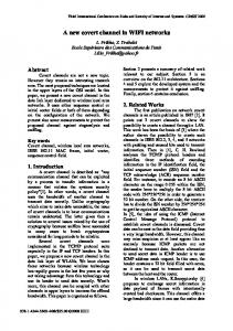
Figure 2.3: CSI signatures for two different human activities (a) Amplitude variations, (b) Raw CSI phase variations, (c) Calibrated CSI phase response. The variations for 30 subcarriers are shown on the left and those of 4 subcarriers are shown on the right. subcarrier (index = -2), the next index reported is -1 and not 0. Then the next subcarriers reported start with index = 1 followed by alternate indices until 27. This is the reason for a linear behaviour in phases across subcarriers 15th to 29th . Then, the break in linearity for the 30th subcarrier is due to index = 28 being reported instead of 29. Since the phases are random (Fig. 2.3b), the PCC maps do not reveal any distinctive patterns in correlations between phases of subcarriers.

2.1.3

OFDM Phase Calibration

Since the raw phase information is not useful to distinguish human activities, a calibration technique [24] can enable phases to become base signals2 in addition to the amplitudes for activity recognition. The measured phase φî for the ith subcarrier can be represented as: 2 Base

signals refer to variations in the amplitude and phase of subcarriers in time from which features are calculated.

17


ki φî = φi − 2π δ + β + Z N

(2.5)

where φi represents the true phase, ki is the subcarrier index in Table 2.1, N is the FFT size (which is 64 in IEEE 802.11n [21]), δ is the timing offset at the receiver, and β and Z denote an unknown phase offset and a measurement noise respectively. Due to several unknowns in equation (2.5), the phases obtained at the NIC is a noisy representation of the true phases. The main idea of the phase calibration technique is to remove δ and β by considering phase across the entire channel bandwidth, which originally consists of 56 subcarriers for a 20 MHz channel. However, since only 30 subcarrier CSIs are reported by the firmware, this is factored into the calculation. Using equation (2.5), the two terms a and b are defined as

a=

b=

1 p

p

φˆn − φˆ1 φn − φ1 2π = − δ kn − k1 kn − k1 N

1 ∑ φˆ j = p j=1

p

∑ φj −

j=1

2πδ pN

(2.6)

p

∑ kj +β

(2.7)

j=1

where p is the number of subcarriers. Referring to Table 2.1, since the subcarrier frequencies are asymmetric, the term ∑ pj=1 k j 6= 0 in equation (2.7). But the authors in [24] have reported that by setting this term to zero, the randomness in raw phases of 802.11n devices can be mitigated to some extent. The calibrated phases φ˜i , are obtained by subtracting a linear term aki + b from equation (2.5) as follows φˆp − φˆ1 1 φ˜i = φî − (aki + b) = φî − ki − k p − k1 p

p

∑ φˆ j

(2.8)

j=1

This process is also referred to as phase sanitization. The calibrated phases of subcarriers corresponding to those measured in Fig. 2.4a are shown in Fig. 2.4b. In Fig. 2.3c, 18


Figure 2.4: (a) Unwrapped CSI phase response , (b) Sanitized CSI phase after calibration. Some parts of (a) are zoomed to show the break in linearity in the unwrapped phase of the 15th and 30th subcarrier. it can be seen the variations in calibrated phases for the different human activities differ. As a result, the calibrated phases are used in addition to the amplitudes as base signals in Wi-HACS. However, the baseline [17] used to evaluate our work only utilized the amplitudes as base signals. Computing the PCC for the calibrated phases of subcarriers in all the TR links, reveal similar observations to those for amplitudes. The calibrated phases of adjacent frequency subcarriers are highly correlated while those of different TR links reveal mostly less correlations.

19


2.2

CSI Time-Series Pre-Conditioning

The goal of pre-conditioning is to address the uneven arrival of packets due to the bursty nature of Wi-Fi transmission, remove underlying temporal variations not instigated by human actions and improve the frequency characteristics of base signals.

2.2.1

1-D Linear Interpolation

The reasons to interpolate the amplitude and phase signals is to enable FFT computations, which require evenly spaced data. This is also important for ‘DeepFalls’ (chapter 4) as unevenly spaced data in time-domain prevent FFT computations to produce spectrograms. Since the dataset in our research is collected at a sampling rate of 100 Hz, we use a 1-D linear interpolation algorithm [8] to evenly arrange data with a spacing of 10 ms. The timestamps of packets are reported as 32 bits by the firmware. By evaluating the difference in the reported time-stamps between two successive packets, the actual elapsed time for each packet arrival can be recorded. The input to the algorithm is packet arrival times, the base signal values and an equal spaced vector consisting of the new time-points to which the CSI values are interpolated.

2.2.2

Hampel Identifier Outlier Removal

The CSI amplitudes and phases contain noises generated by internal state transitions such as transmission power and rate adaptations, and thermal noises in the devices [25]. As a result, these introduce variations and outliers to the base signals which are not caused by human presence. The outliers are indicated by ‘circles’ in the CSI amplitude waveforms in Fig. 2.5a. In the figure, the most obvious outlier can be seen, for instance at t = 5s. The other outliers in Fig. 2.5a are declared by the Hampel Identifier algorithm [26].

20


(b)

35

35

sub#1 sub#15 sub#30

30

Amplitude (dB)

Amplitude (dB)

30

25

20

15

sub#1 sub#15 sub#30

25

20

0

2

4

6

8

Time (s)

10

12

14

15

0

2

4

6

8

10

12

14

Time (s)

Figure 2.5: Effect of Hampel Outlier Removal on three subcarriers: (a) Raw CSI Amplitude waveforms with outliers denoted by ’black circles’, (b) Hampel filtered CSI amplitude waveforms. The algorithm works as follows. For each value x of the base signals, the median of a window consisting of x and m/2 neighboring points on each side, is computed. Then the standard deviation of x about its window median is calculated using the Median Absolute Deviation (MAD). If x differs from the median by more than a predefined number of MAD, its value is replaced by the median. In other words, the Hampel Identifier declares discrete values as outliers outside the interval [µ − γ ∗ σ , µ + σ ∗ γ], where µ and σ represent the median and MAD respectively and γ is dependent on the application and has a default value of three. In our research, we varied the value of m and kept the default value of γ = 3. By varying m in increments of 5, we observed whether the most obvious outliers are detected. In the end, m = 20 seemed a good choice for the number of points along with x.

21


30

20 0.5

1

1.5

2

2.5

0

3

0

Time (s) (c)

40 20

0

10

20

30

Frequency (Hz)

0.5

40

50

1

1.5

2

2.5

3

Time (s) (d)

1.5

Amplitude

60

Amplitude

Hampel Filtered Subcarrier linear regression

5

-5 0

0

(b)

10

Hampel Filtered Subcarrier linear regression

Amplitude

Amplitude

40

1 0.5 0

0

10

20

30

40

50

Frequency (Hz)

Figure 2.6: Effects before and after de-trending CSI waveforms: (a) Hampel Filtered subcarrier for walking activity, (b) De-trended waveform of (a); One-sided amplitude spectrum of FFT for (c) before de-trending, (d) after de-trending

2.2.3

De-trending Subcarriers to avoid spectral distortion

The CSI base signals sometimes display a trend, which can be visualized as a positive or negative slope over the length of the signal. This effect is mostly observed during human activities which include vertical hops such as squatting, jogging, etc. But in a few cases, this trend is also observed in non-hoping activities such as walking or sitting down. These effects on the amplitude signal during a walking activity can be seen in Fig. 2.6. In Fig. 2.6a, a linear regression line has been plotted to visualize this trend. The frequency associated with the trend is lower than the lowest (fundamental)3 frequency in the spectrum. The energy from this trend is leaked to that of the lower frequencies, thereby distorting the lower part of the spectrum [16]. This distortion can be minimized by subtracting the data from the linear regression line, also known as de-trending. This is important in our research because some amplitudes of dominant frequencies will be 3 fundamental

frequency is 1/T , where T is the duration of the window [16]

22

Chapter 2. Wi-HACS: A Wi-Fi based Human Activity Classification using OFDM Subcarriers used as features in Chapter 3. Furthermore, de-trending can also remove the zeroth or DC frequency component shown in Fig. 2.6c. This is because the zeroth frequency component is the mean of the signal based on the following DFT equations [27] L−1

X[ f ] =

∑ x[l] exp− j2πl f

(2.9)

l=0

where L is the length of the signal. At the DC frequency, the equation becomes L−1

X[0] =

∑ x[l]

(2.10)

l=0

As a result, the DC frequency is simply the mean of the signal. Hence by de-trending, the lower spectral distortion is minimized and the DC frequency is removed.

2.2.4

Effect of zero-padding in FFT computations

Since the frequency resolution (number of frequency points) of the FFT is determined by the length of the time-series, it is possible to increase frequency resolution by adding more time points [28]. This can be done by a process known as zero-padding, which adds extra zeros at the end of the time-series. There are two main reasons to zero-pad the CSI base signals in Wi-HACS: (i) Since the base signals of some activities, for example sitting and standing, are similar and share the same FFT profiles, increasing frequency resolution can improve features derived from FFT, in particular the autospectrum. Because when frequency resolution is improved, the frequencies smeared in the FFT profile can be distinguished better. (ii) It can improve FFT processing times, as this algorithm is most efficient if the input time-series has a length corresponding to a power of two. The improvements in resolution due to zero-padding can be observed in Fig. 2.7.

23


1.2

1) two frequencies smeared together

0.8 2) four frequency points very close to each other

0.6 0.4 0.2 0

1) two distinct frequencies with higher amplitude

1

Amplitude

Amplitude

1

(b)

1.2

0.8

2) four frequency points separated with one very distinct frequency

0.6 0.4 0.2

0

10

20

30

40

50

0

0

10

Frequency (Hz)

20

30

40

50

Frequency (Hz)

Figure 2.7: FFT profile of the walking activity (a) before, (b) after zero padding

2.2.5

Tapering CSI waveforms to prevent edge artifacts

When the FFT is applied to a data vector of finite duration T, the periodicity assumption in Fourier analysis [16] creates a step discontinuity at y(T) unless y(0) = y(T ). This results in leakage of spurious energy to many frequency bands and hence distorts the Fourier spectrum. To understand this from a mathematical point of view, let us assume a time series y(t) whose duration is from −T /2 ≤ t ≤ T /2. Assuming a window function w(t) is defined as

w(t) =

   1, for −T /2 ≤ t ≤ T /2.

(2.11)

  0. otherwise If wˆ and Yˆ are the Fourier transforms of w(t) and y(t), then the Fourier transform of w(t)Y (t) is the convolution of wˆ and Yˆ . If the window function is rectangular (equation (2.9)), then its Fourier transform wˆ being a sinc function and the convolution of wˆ and Yˆ produces spurious energy leakages into lower frequency bands [16]. To prevent these edge discontinuities, it is necessary to multiply the data windows by a taper before taking its Fourier transform. The taper is a function that decays smoothly to zero near the ends of each window. Although spectral leakage cannot be completely prevented, it can be 24

Chapter 2. Wi-HACS: A Wi-Fi based Human Activity Classification using OFDM Subcarriers significantly reduced by altering the shape of the taper function. The cosine taper with different taper ratio, (0 ≤ a ≤ 1), in time and frequency domains is illustrated in Fig. 2.8. The mathematical form of this taper is:

c(t) =

   π 1  1 − cos( t) ,  2 a   

for 0 ≤ t ≤ a.

1. for a ≤ t ≤ (1 − a).        1 1 − cos( π (1 − t)) , for (1 − a) ≤ t ≤ 1 2 a

(2.12)

By increasing a the power leakage from a spectral peak to adjacent frequencies is decreased. Referring to Fig. 2.8, the ideal taper to consider would be the Hann taper which results in the quickest power decay in frequency domain. However, using this window would truncate a lot of data at the start and end of the window, therefore losing signal information. Considering the other extreme when a=0% or the rectangular window, the original time-series data is completely preserved, however it results in the slowest decay of frequency across the bandwidth. This results in a time and frequency trade-off and hence it is important to balance the loss of signal in time-domain with the power decay in the frequency domain. The amplitude base signal for the walking activity is multiplied by cosine tapers for various values of a and the FFT profiles are computed for each case for illustrations in Fig. 2.9. It is observed when a is increased, the window shape resembles more like a ‘cosine bell’ and hence increases the bandwidth, reducing the amount of spectral leakage and thus improving the resolution of adjacent low-frequency spectral components. This is essential to the development of Wi-HACS because all human activities give rise to low-frequency components but the energy across these components vary for different activities. However, the amplitude of FFT profiles of the tapered signals decrease with increasing tapering ratio. This is because increasing a has the drawback of attenuating valid data at the beginning

25

Chapter 2. Wi-HACS: A Wi-Fi based Human Activity Classification using OFDM Subcarriers Window Viewer

(a) Time domain

(b) Frequency domain

100

rectangular (a=0%) cosine taper (a=25%) cosine taper (a=50%) cosine taper (a=75%) Hann (a=100%)

1 50

Magnitude (dB)

Amplitude

0.8 a=0% (rectangular)

0.6

a=25% a=50% a=75%

0.4

a=100%(Hann)

-50 -100

0.2 0

0

20

40

60

80

100

120

-150

Samples

0

0.2

0.4

0.6

0.8

Normalized Frequency (×π rad/sample)

Figure 2.8: (a) Time-domain and (b) FFT profile of the cosine taper with various tapering ratios and end of the time-series. In our research work, we set the value of a to be 5% to ensure a good balance between the time and frequency trade-off.

2.3

Discrete Wavelet Transform (DWT) based Noise Attenuation for CSI signals

In this section, the noise attenuation techniques commonly used in CSI based HAR will be covered. After identifying their limitations, the DWT will be introduced as a de-noising technique. The concept of DWT as dyadic filter banks, followed by selection of mother wavelet and decomposition levels, is explained. Finally, the thresholding technique and the threshold value needed to reconstruct the signals from filter decompositions will be given.

26

Chapter 2. Wi-HACS: A Wi-Fi based Human Activity Classification using OFDM Subcarriers (a) Time-domain (a=5%)

5

(b) Frequency-domain (a=5%)

1.5

Hampel Filtered + De-trended Hampel Filtered + De-trended + Tapered

Amplitude

Amplitude

10

0 -5

1 0.5 0

0

0.5

1.5

2

2.5

3

0

Time (s) (c) Time-domain (a=25%)

10 5 0 -5

10

20

30

40

50

Frequency (Hz) (d) Frequency-domain (a=25%)

1.5


Amplitude

Amplitude

1

1 0.5 0

0

0.5

1.5

2

2.5

3

0

Time (s) (e) Time-domain (a=50%)

10 5 0 -5

10

20

30

40

50

Frequency (Hz) (f) Frequency-domain (a=50%)

1.5


Amplitude

Amplitude

1

1 0.5 0

0

0.5

1

1.5

2

2.5

3

Time (s)

0

10

20

30

40

50

Frequency (Hz)

Figure 2.9: The FFT profiles of the amplitude signal during the walking activity multiplied by cosine tapers of various tapering ratios (a) Time domain and (b) Frequency domain for a=5%, (c) Time-domain and (d) Frequency domain for a=25%, (e) Time domain and (f) Frequency domain for a=50%.

2.3.1

Limitations in time and frequency based noise attenuation techniques in CSI systems

In current CSI based HAR literature, the noise attenuation techniques can be categorized into time and frequency based approaches. The time-domain approaches are the median filtering [10] and the Principal Component Analysis (PCA) de-noising [25]. The frequency domain approaches are low-pass [29] and band-pass filtering (Butterworth) [6]. In [28] it is stated that the above time-domain approaches can distort the signal and result in loss of some vital high frequency components. In PCA based de-noising, the first Principal Component (PC) is removed as it is considered to represent the highest noise variance. The disadvantage of this technique is that it also removes most of the information (vari-

27

Chapter 2. Wi-HACS: A Wi-Fi based Human Activity Classification using OFDM Subcarriers ance) representing the human activity. In complex environments where relatively less information about human activities is conveyed by CSI signals, this de-noising technique can remove almost all useful information. Frequency domain approaches in CSI-based HAR are mostly “out-of-band” filtering techniques, where noises in the passband are not eliminated. Since CSI signals have noise in all frequency bands [30], we propose an “in-band” noise-filtering technique based on the DWT to eliminate noise in all frequency bands, while preserving high frequency components. This is advantageous because the CSI base signals consist of rapid variations in very short durations such as during a change in activity, and are preserved after DWT de-noising.

2.3.2

The Discrete Wavelet Transform (DWT) as a dyadic filter bank

The DWT can be realized as a dyadic filter bank, where filters of different cutoff frequencies are used to analyze the signal at different scales. The signal is passed through this bank to obtain high (details) and low frequency (approximation) components respectively. The procedure starts with passing the signal through a bank of half-band digital lowpass and highpass filters whose impulse response are h[n] and g[n] respectively, as shown in Fig. 2.10. The next step involves downsampling the signal by 2 since the BW of the bandlimited signal is now halved and according to Nyquist, the sampling rate is now half of the initial rate. Therefore, the length of the signal at this stage is L2 . It is important to note that the low-pass filtering removes the higher half-band information without altering the scale. The scale is changed due to the downsampling process. Since resolution is related to the number of points (information) in the signal, it is affected by the filtering operation. Thus, the resolution is decimated by 2 after the filtering operation and the scale is doubled after the downsampling operation. Therefore the DWT analyzes the signal at different frequency bands with different resolutions. The lowpass and highpass filters

28


Figure 2.10: (a) The subband coding algorithm in DWT [31] correspond to the two functions of DWT: scaling and wavelet respectively. At each level of the DWT, the decomposition reduces the time resolution by two (as half the number of samples characterize the signal at the previous stage). In contrast, the frequency resolution at each stage doubles, since the frequency band at each stage spans only half of the bands at the previous stage. This procedure is referred to as subband coding [31] and is illustrated in Fig. 2.10. By using this technique, at low frequencies, the frequency resolution is preserved, while at higher frequencies, the time resolution is preserved. The 3-level DWT decomposition of CSI amplitude signal for the walking activity, utilizing the ‘Daubechies’ (db-8) [32] wavelet is illustrated in Fig. 2.11. The choice of db-8 as mother wavelet is adopted from [33], in which the authors have shown it is the optimal choice for de-noising non-stationary Electrocardiogram (ECG) signals. Although our base signals are different 29


(i) Pre-conditioned CSI Amplitude

20

Amplitude

(0-50Hz)

0

-20 0

2

4

6

8

10

12

14

Time(s) (ii-a) Level 1 Approximation coefficients

(ii-b) Level 1 Detail coefficients

20

Amplitude

Amplitude

20

(0-25Hz)

0 -20

(25-50Hz)

0 -20

0

100

200

300

400

500

600

700

800

0

100

200

(iii-a) Level 2 Approximation coefficients

20

(0-12.5Hz)

0 -20

400

500

600

700

800

(iii-b) Level 2 Detail coefficients

20

(12.5-25Hz)

0 -20

0

50

100

150

200

250

300

350

400

0

50

100

Number of points

150

200

250

300

350

400

Number of points

(iv-a) Level 3 Approximation coefficients

(iv-b) Level 3 Detail coefficients

20

Amplitude

20

Amplitude

300

Number of points

Amplitude

Amplitude

Number of points

(0-6.25Hz)

0 -20

(6.25-12.5Hz)

0 -20

0

50

100

Number of points

150

200

0

50

100

150

200

Number of points

Figure 2.11: The DWT decomposition structures for CSI amplitude during ‘walking’ event (i) Pre-conditioned amplitude, (ii)-(iv) representing levels 1-3 respectively and (a) and (b) denoting approximations and details for each level. from ECG signals, they are nonetheless non-stationary. Since the main objective of our research is to improve the classification performance of HAR, we leave the exploration of other wavelet functions for future work. The decomposition level was chosen to be 3 based on previous spectrogram results given in [12] and [34]. In our research, we define three sets of activities in our data: in-place (sit and stand), out-of-place (walk, squat, jog) and fall-events (fall-from walking and sit-from walking). According to [12] the “in-place” activities occupy (0-5 Hz); the “out-of-place” and “fall-events” occupy the entire spectrum (0-50 Hz). In Fig. 2.11, the approximation and detail coefficients at each level of decomposi-

30

Chapter 2. Wi-HACS: A Wi-Fi based Human Activity Classification using OFDM Subcarriers tion can be seen. The x-axis represents the number of data points instead of time, as it decreases by half in subsequent decompositions as a result of downsampling. A further decomposition would produce level-4 approximation coefficients spanning (0 - 3.125 Hz) which would ideally represent very subtle activities such as making a phone call while sitting. However, since in our measurements, we do not include such activities, the DWT decomposition is set to level 3. By the process of inverse discrete wavelet transform (IDWT), the signal can be reconstructed. However in DWT de-noising, the detail coefficients are thresholded before applying the IDWT. This is the scope of the following subsection.

2.3.3

Thresholding methods and value selection

In the first step of the DWT noise attenuation, the signal is decomposed using a mother wavelet into pre-determined decomposition levels W resulting in approximation and detail coefficients at each level (Fig. 2.11). Then, thresholding is applied to the detail coefficients from level 1 to W . Finally, the noise-attenuated signal is constructed using the original approximation coefficients in level W and the thresholded detail coefficients in levels 1 to W [35]. The two most common methods of thresholding the wavelet coefficients are: hard thresholding and soft thresholding [35]. In both methods, the wavelet coefficients with magnitude less than the threshold value are set to zero. The difference between these two operations lie in how the magnitude of wavelet coefficients greater than the threshold are manipulated. In soft thresholding, the magnitude of coefficients greater than the threshold are shrunk towards zero by subtracting the threshold from the coefficient. In hard thresholding, the coefficients greater than the threshold remain unchanged [35]. The two equations defining hard and soft thresholding [36] respectively, are given as

31


g w j,i =

   w

j,i

  0

g w j,i =

: |w j,i | ≥ λ j .

(2.13)

: |w j,i | < λ j

   sgn(w j,i )(|w j,i | − λ j ) : |w j,i | ≥ λ j .   0

(2.14)

: |w j,i | < λ j

g where λ j is the threshold value, w j,i amd w j,i are the noisy and denoised wavelet coefficients, respectively, at the jth decomposition level and the ith location of the detail component, and j ≤ W . Hard thresholding is more suitable when the detail coefficients represent a signal or a noise. In contrast, soft thresholding performs better when the detail coefficient contain both signal and noise [36]. Since, the detail coefficients of our CSI signals contain both signal and noise, we use the soft thresholding technique. In DWT de-noising, there exists several methods [37] to estimate the threshold value. Since the authors in [38] have experimentally shown the universal threshold [39] is the simplest and most effective method, it has been adopted in our work. The universal threshold is given by

λU = σ

p 2 log(L)

(2.15)

where L denotes the length of signal, and σ is the noise standard deviation. Since the noise in our data is not known, the first-level detail coefficients D1 can be used to estimate σ [35] using the following equation

σ=

median(|D1 |) 0.6745

(2.16)

After thresholding the detail coefficients (levels 1 to 3), and reconstructing the signal using these and the third level approximations, the noise-attenuated version of the CSI base sig-

32


(a) Original Signal walk

20

jump

stand

walk

10 0 -10 -20

standing up from sitting

0

4

6

8

10

12

jump


0

2

4

6

jump

stand

walk

0

-20


0

4

6

8

Time(s)

10

12

14

walk

20

14

jump

stand

walk

10 0 -10

2

12

(d) Discrete-Wavelet Transform De-noising

10

-10

10

30

Amplitude

Amplitude

walk

8

Time(s)

(c) Low-pass Filtered

20

walk

0

Time(s) 30

stand

10

-20

14

walk

20

-10

2

(b) Median Filtered

30

Amplitude

Amplitude

30

-20


0

2

4

6

8

10

12

14

Time(s)

Figure 2.12: Various de-noising algorithms applied to pre-conditioned CSI-amplitude time-series for a series of activities:(a) Original pre-conditioned signal, (b) 5-point median filtering, (c) Butterworth Low-pass filter with cutoff frequency at 30Hz, and (d) 3-level ‘db-8’ DWT based de-noising. nals can be constructed. The pre-conditioned amplitude base signal after applying various de-noising techniques for a series of human activities is shown in Fig. 2.12. The 5-point median filtering algorithm [40] do not preserve sharp transitions in the signal. This is because any short transition usually appears to be a large value in the median-window and is replaced by the median value. As a result abrupt changes in signals are smoothed and high frequency components are lost. This can be observed in Fig. 2.12b in the region of 600 ms, where spikes in the original signal (Fig. 2.12a) are flattened. Although Butterworth low-pass filtering can maintain these sharp transitions, as observed in Fig. 2.12c, it is an out-of-band filtering technique, in which all high frequency components outside the cutoff are lost and noises within passband are not eliminated. In contrast, the DWT-based approach removes noises from all frequency bands and retains high frequency components.

33


Ratio of total variance explained by mode

0.8 modes corresponding to T1-R1 modes corresponding to T1-R2 modes corresponding to T2-R1 modes corresponding to T2-R2

0.7 0.6 0.5 0.4 0.3 0.2 0.1 0

0

5

10

15

20

25

30

mode number

Figure 2.13: The variance of eigenvalues (modes) after the eigendecomposition of the covariance matrices for each transmit-receive link.

2.4

Principal Component Analysis (PCA) Dimension Reduction

Since the CSI amplitude and phase signals correspond to 120 dimensions for two TR links, we use PCA [22] to reduce the number of correlated signals. In the baseline work, the authors averaged the signals into one signal per link. Since in their work only amplitude is used, the total dimensions were 60, and hence reduced to only two base signals. From our analysis in section 2.1.1, we demonstrate subcarriers further away in frequencies show little to no correlation and hence averaging is not the optimal choice. The following describes the PCA process to choose the optimal number of PCs to represent our data, where Xi represents the ith TR link: (i) Mean removal: Since the signals are de-trended in the pre-conditioning step, the mean is already subtracted from each subcarrier in Xi .

34

Chapter 2. Wi-HACS: A Wi-Fi based Human Activity Classification using OFDM Subcarriers (ii) Covariance matrix estimation: Since Xi has 30 subcarriers (30-dimensional), the covariance matrix for each link, Yi = XiT Xi is of dimensions 30 x 30.

(iii) Eigen-decomposition: Since Yi is a square matrix, the eigenvectors Wi corresponding to eigenvalues λi can be computed. The columns of Wi are "ordered" such that the 1st column (1st "PC" or 1st "loading") corresponds to the highest eigenvalue followed by the 2nd column (2nd "PC" or 2nd "loading") corresponding to the second highest eigenvalue, and so on.

(iv) Optimal number of PCs: This is based on the number of eigenvalues used to represent a good variance of the data. From Fig. 2.13, it can be observed the first 3 PCs represents ≈ 90% of the variance of the data. The data in this case is a matrix, whose columns represent the subcarriers and the rows represent the values of these subcarriers at each time point. Since our research objective is to improve classification accuracies, we trained and tested the Support Vector Machine (SVM) classifier using features calculated from different numbers of amplitude and phase PCs. Our classifier results indicated that if the classifier was trained using features from more than three PCs, the cross-validation results did not improve. Therefore, the CSI time-series in our research is reduced to NT x x NRx x 3 = 1 x 2 x 3 = 6 amplitude and 6 phase base signals.

2.5

Adaptive Windowing for CSI-signal Segmentation

One of the key challenges in CSI-based HAR systems is to accurately segment the start and end of a human activity from CSI signals. This is needed to calculate features from each window for classification. The methods commonly used in existing CSI-based HAR are ‘event-detection’ or ‘fall-event segmentation’. In the event detection method [41], 35

Chapter 2. Wi-HACS: A Wi-Fi based Human Activity Classification using OFDM Subcarriers the sliding window first determines whether there is a human activity and if so, continues with the feature extraction and classification algorithms. If no human activity is detected, the window is slid after a pre-defined number of data points. The limitation of such a technique is since different human activities may be performed for different durations, a non-adaptive window can result in missing a change in human activity. In fall-event segmentation method, the signal is segmented to only determine the start and end of a ‘fall-event’ such as in [10], [11] and[12]. Although the latest CSI-based fall detector [12] reports a segmentation accuracy of 100%, this technique cannot distinguish the start and end of non-fall activities. Since Wi-HACS is designed to classify both fall-events and other activities, the above two methods are not suitable. Therefore we propose an adaptive windowing segmentation based on the amplitude of FFT coefficients. As described in section 2.3.5, different categories of human activities occupy different spectral bands. Therefore an activity segmentation can be based on analyzing the spectral components on each window. However, there are two challenges with such an approach: 1) Out-of-place activities such as walking occupy the entire spectral band in the entire window, hence part of its spectrum overlaps with in-place activities such as sitting or standing. 2) Fall events which consist of true falls and fall-like activities (sitting down from walking) occupy different spectral bands at different time periods in the activity window. Hence, we propose an adaptive sliding window to overcome these problems. From our empirical observations, amplitudes of frequencies ranging between (3-25 Hz) is sufficient to determine the segmentation. In every determination of activity segments, we propose two windows of length 200 (2 s) with 1 s overlap. We define low frequency ( fL ) to be from 3-10 Hz and high frequency ( fH ) from 10-25 Hz. For demonstration purposes, let’s assume the lengths of first and second window are (α2 − α1) and (β 2 − β 1) respectively. In each window any frequency content with an amplitude less than 0.2 is

36

Chapter 2. Wi-HACS: A Wi-Fi based Human Activity Classification using OFDM Subcarriers discarded. This is because for in-place activities as defined in section 2.3.5, most of the energy (amplitude) of FFT coefficients are concentrated within 0-5 Hz and few coefficients with very low amplitudes (< 0.2) are present outside this band. Since in-place activities contain fL and out-of-place activities contain both fL and fH , the signal window is adapted based on the following four cases:

Case 1: Both windows w1 and w2 contain fL : This means both windows contain in-place activities (sit or stand). In this case the two windows are left unchanged and is further processed individually for feature extractions and classification. Any change in activity (sit to stand or vice-versa) is based on the classification output.

Case 2: w1 contains fL and w2 contains both fL and fH : This implies there is a change in activity from in-place to out-of-place and hence features will be calculated from each window and classifications will be made individually.

Case 3: Both windows w1 and w2 contain both fL and fH : In this case, a third window w3 of length 200 is computed for the next part of signal without any overlap. This is done to estimate the frequency components of w3 to identify whether a change in activity has taken place in w2. This is important because as explained above, fall-events first occupy higher spectral bands corresponding to a rapid movement followed by occupation of lower spectral bands corresponding to the person lying down. Thus there will be two specific cases in this regard: (i) If w3 contain fL : Identify that there is a change in activity which occurred within w2 and hence merge w2 and w3 to form w4 and calculate features from this combined window

37


Open door and enter room No human presence

Perform 4 squats

Sit down Walk around

Jog in room Falldown

Stand still

Stand up

15 10

Amplitude (dB)

Window 1

5

Window 2 Window 3

0 -5 -10 0

Two windows individually processed

10

20

30 Time (s)

Three windows with w2 compared with w3. Since w2 has fL and fH and w3 has fL these two windows will be combined to form w3

40

50

Fall-event: both windows combined for further processing

Figure 2.14: Adaptive Windowing based on the amplitude of FFT coefficients of length: 300 and the w1 of length: 200 separately. In this case w1 will consist of an out-of-place event and w4 will consist of a fall-event. (ii) If w3 contain both fL and fH : This implies the out-of-place activity is continuously being performed in w1, w2 and w3. Hence features will be calculated individually from w1 and w2. The w3 will now be labelled as w1 and followed by the next window w2 overlapping 1s of w1 as the usual case and then the two windows will be evaluated on a case by case basis.

Case 4: w1 contains fL and fH and w2 contains fL : This indicates a ‘fall-event’ has taken place, which can either be a true-fall or a fall-like 38

Chapter 2. Wi-HACS: A Wi-Fi based Human Activity Classification using OFDM Subcarriers activity. In this case the two windows will be merged whose length will now be (β 2 − α1) to determine if it’s a true-fall or fall-like activity. The adaptive windowing for these cases can also be visualized in Fig. 2.14. The discussions listed above are true for both amplitude and phase base signals.

39


2.6

Summary

In this chapter, the foundations behind Wi-HACS were reported. The concept of CSI and the base signals: amplitudes and phases were introduced. We analyzed the correlations between subcarriers which are adjacent to each other, and also far away in frequencies. We observed the correlations between adjacent subcarriers are mostly correlated. We also observed some interesting patterns in the correlations between subcarriers which are further away in frequencies. These observations results in novel features which improves the classifications, specially in complex environments. We will discuss more about these features in Chapter 3. Since the phases are extremely random, a phase calibration algorithm was used to show that phase signatures can also be used as base signals, hence providing additional channel signatures corresponding to human activities. Essential pre-conditioning steps were taken to reduce the base signal artifacts induced by hardware imperfections. Since we derive some features from FFT (details in Chapter 3), de-trending, zero-padding and tapering techniques were explored to improve the FFT profiles of different human activities. The DWT noise attenuation was proposed to overcome the limitations of the de-noising techniques used in current CSI-HAR systems. The PCA algorithm was used to reduce the number of correlated subcarriers in each TR link. Since there is no segmentation method that works for both falls and non-fall activities, we proposed an adaptive windowing technique capable of segmenting both types of activities.

40

Chapter 3 Wi-HACS: Classification and Performance Analysis The main objectives of this chapter are to evaluate the proposed signal processing and novel features and compare our results against a baseline. We begin by introducing features adopted from the baseline and explain novel features based on subcarrier correlations and dominant frequencies in the autospectrum of base signals. We then discuss the approach taken to tune the parameters in a multi-class SVM classifier. This is followed by a description of procedures taken to collect the data. The performance metrics used to evaluate Wi-HACS are also defined. We present the method used to choose the optimal number of amplitude and phase Principal Components (PCs). We assess whether the features extracted from DWT and Hampel filtered signals improve classifications by comparing the results using features from de-noised signals with those obtained from raw signals. We also evaluate whether our proposed features improve classification results. We then compare our work with a baseline and discuss the results. Finally, we present the results of a one-tailed paired t-test to determine whether our improvements are statistically significant.

3.1

Feature Extraction

In this section, we will outline the features adopted from the baseline [17] and describe novel features which are derived from the subcarrier correlations and the amplitudes of 41

Chapter 3. Wi-HACS: Classification and Performance Analysis frequencies in the autospectra of base signals.

3.1.1

Features adopted from baseline

The features utilized in the baseline are commonly used in wearable-based HAR systems [2]. The features adopted can be categorized into time and frequency based. The time domain features are based on statistics: (i) Normalized Standard Deviation, (ii) Skewness, (iii) Kurtosis, (iv) Interquartile range, and (v) Median Absolute Deviation. The frequency domain feature is the Normalized Entropy or Power Spectral Entropy [42], which estimates the disorder measure of time-series data in frequency domain. It is calculated by the following steps:

(i) Calculate the FFT of the signal, S( fi ), where fi is the frequency corresponding to the ith data point.

(ii) Calculate the Power Spectral Density (PSD) of the signal by squaring the amplitude spectrum and scaling it by the length L of the signal ˆ fi ) = 1 |S( fi )|2 P( L

(3.1)

ˆ fi ) (iii) Normalize the PSD, P( pi =

ˆ fi ) P( L

(3.2)

ˆ fi ) ∑ P(

i=1

(iv) Calculate the normalized entropy as L

E = − ∑ pi ln pi

(3.3)

i=1

42

Chapter 3. Wi-HACS: Classification and Performance Analysis The value of L depends on the type of activity segmented; for fall-events, L = 300 (3 s) and for in-place and out-of-place activities, L = 200 (2 s). In addition to the adopted features, we identified two measures: Correlations in timedomain and Autospectrum in frequency domain from which a total of 120 novel features are proposed. The former is calculated by measuring the PCC across a specific group of subcarriers and the latter is calculated from the optimum number of amplitude and phase PCs. Once the autospectrum of these PCs are calculated, the frequencies corresponding to the most dominant amplitudes are taken as features. The improvements in classification results with our proposed features are experimentally measured and reported in section 3.4.4.

43

Chapter 3. Wi-HACS: Classification and Performance Analysis

Figure 3.1: PCC correlation matrices of amplitude of subcarriers of the same T-R link after signal pre-conditioning. Area of interest corresponds to the correlation values taken as features: Out-of-place activities: (a) Walking, (b) Jogging, and in-place activities: (c) Sitting and (d) Standing. The colour bar represents the correlation values.

3.1.2

Proposed features based on subcarrier correlations

The correlation matrices are obtained by computing the PCC between the amplitudes of 30 subcarriers for one TR link during different human activities. We observe unique correlation patterns across a group of subcarriers, during different human activities for a given environment. Referring to Fig. 3.1, the area of interest in each symmetrical correlation matrix reveals distinctive patterns between subcarriers from indices #5 − 15 with the ones from #25 − 30. Specifically, these correlation patterns show relatively higher correlation

44

Chapter 3. Wi-HACS: Classification and Performance Analysis values for out-of-place activities, walking and jogging, and lower values for in-place activities, sitting and standing. Although these observations are also valid for the phase signals, we derive these features from only the amplitude signals, to reduce overfitting.

3.1.3

Proposed features based on autospectrum

The autospectrum [16] of a signal s(tn ) represents the variance in terms of its Fourier coefficients. The following derivations will establish this relationship. The discrete Fourier series representation of s(tn ), where n = 1, 2, ..., L, sampling interval ∆t = T /L, and the observations are made at time tn = n∆t, is given by M 1 L s(tn ) = ∑ s(tn ) + ∑ am cos(ωmtn ) + bm sin(ωmtn ) L n=1 m=1

where M is the largest integer ≤ L/2, ωm is the angular frequency given by ωm =

(3.4) 2πm L ,

and

am and bm are the Fourier coefficients given by 2 L am = ∑ (s(tn ) cos(ωmtn )), L n=1

m = 0, 1, 2, ..., M

(3.5)

2 L ∑ (s(tn) sin(ωmtn)), L n=1

m = 0, 1, 2, ..., M

(3.6)

bm =

Denoting s(tn ) as sn , the variance of the time-series s is given as

var(s) =

1 L ∑ sn − s)¯ 2 L n=1

(3.7)

where s¯ represents the mean of s. Using Equation (3.4) the variance can be written as

var(s) =

i2 1 L h M a cos(ω t ) + b sin(ω t ) mn m mn ∑ ∑ m L n=1 m=1

(3.8)

45

Chapter 3. Wi-HACS: Classification and Performance Analysis Since the sine and cosine functions have orthogonality properties: L

L

∑ cos(ω ptn) cos(ωqtn) = 2 δ pq

n=1 L

L

∑ sin(ω ptn) sin(ωqtn) = 2 δ pq

(3.9)

n=1

L

∑ cos(ω ptn) sin(ωqtn) = 0

n=1

where δ pq is the Kronecker delta function. Using the equations in (3.9), the variance in Equation (3.8) can be written as

var(s) =

1 M 2 ∑ (am + b2m) 2 m=1

(3.10)

The autospectrum, Am , can be visualized as the energy contained in the frequency bands

Am =

L∆t 2 (a + b2m ) 4π m

(3.11)

where ∆t represents the sampling period. Therefore, the total variance can be written in terms of the autospectrum as follows M

var(s) =

∑ Am∆ω

(3.12)

m=1

with

∆ω =

2π L∆t

(3.13)

This autospectrum Am is computed from the optimum number of amplitude and phase PCs from each TR link. In each spectrum, the frequencies corresponding to the 1st five dominant amplitudes are recorded as features. The number of dominant amplitudes was

46

Chapter 3. Wi-HACS: Classification and Performance Analysis Feature

Domain

Subcarrier Correlations

Time

Autospectrum

Frequency

Normalized Standard Deviation Skewness Kurtosis Inter-quartile Range Median Absolute Deviation Normalized Entropy

Base Signal

# of T-R links

# of features

1

60

2

60

2

12

2 2 2

12 12 12

Time Time Time

Amplitude of subcarriers indexed 5-15 with 25-30 First five peaks of 3 Amplitude and 3 Phase Principal Components 3 Amplitude and 3 Phase Principal Components " " "

Time

"

2

12

Frequency

"

2 Total # of features

12 192

Time

Table 3.1: Extracted Features for Wi-HACS chosen by trial and error. A table of the features used along with the number of base signals and TR links are given in Table 3.1. In Table 3.1, the first two rows represents the novel features while the remaining rows represent the adopted features.

47


3.2

Multi-Class Support Vector Machine (SVM) Classification

The Support Vector Machine (SVM) [43] is an algorithm that can achieve high generalization, meaning that test data can be classified correctly, by maximizing the margin between the hyperplane and the nearest feature vector. It can also classify labels/classes which are not linearly separable, by the use of a kernel function. Given a training dataset D = {(x1 , y1 ), (x2 , y2 ), ..., (xm , ym )}, where xi is a n-dimensional feature vector, yi is the class/label to which the feature vector belongs, with a value of a 1 or -1, the soft margin SVM algorithm solves the following optimization problem

min

w,b,εi

s.t.

m 1 ||w||2 +C ∑ ξi 2 i=1

yi (w · xi − b) ≥ 1 − ξi ,

∀(xi , yi ) ∈ D

(3.14)

ξi ≥ 0 where ξi measure the degree of misclassification, and C is a tunable parameter, that determines the tradeoff between the margin size and amount of error in training. The optimization problem can be solved using Lagrange multipliers and the dual problem can be used to solve for the optimal hyperplane separating the classes. When the classes are not linearly separable the non-linear SVM can be used, which consists of two steps: 1) The input feature vectors are transformed into high-dimensional space where the training data can be linearly separated, 2) then the soft-margin SVM is used to find the hyperplane of maximal margin in the new feature space. A kernel function is used to compute the dot product between feature vectors as if they have been transformed to a higher dimensional space, without actually transforming the vectors. The kernel used in our SVM classifier is the Radial Basis Function (RBF) Kernel, as it has proven to be a good choice [44]. The equation 48

Chapter 3. Wi-HACS: Classification and Performance Analysis for RBF kernel is K(xi , x j ) = exp(−γ||xi − x j ||2 ), where K(xi , x j ) is the kernel function that computes the dot product of the feature vectors and γ > 0 is the kernel parameter. A large gamma leads to high bias and low variance models, and vice versa. Therefore, two parameters in the SVM classifier needs to be tuned: C and γ. The strategy used to find good values for these parameters are adopted from [44], in which it suggests to scale features and then use cross-validation to find the parameters. The feature scaling step in SVM is important as features with very large numerical values dominate the ones with smaller numerical values [44]. All training and testing data in our research were normalized to lie in the range [0,1].

3.2.1

Cross-validation and Grid-search

Since the optimal values for the C and γ are not known beforehand, a grid-search technique was used. The goal of finding these optimal values is to minimize the training and validation losses. In our research, the data are split into training, validation, and testing. The training and testing data were taken from two different regions of the experimental rooms, as illustrated in Fig. 3.2. A 10-fold cross validation is performed on the training data. Thus, each instance of the entire training set is predicted once resulting in a crossvalidation accuracy. This was done to prevent overfitting. The grid-search on C and γ was done using cross-validation. By trying different combinations of (C, γ), the one which resulted in the highest cross-validation accuracy was selected. After applying grid-search and cross-validation, the optimal values were obtained as C = 0.025 and γ = 0.03125, C = 0.03 and γ = 0.04, and C = 0.01 and γ = 0.04 for the three environments in Fig. 3.2 respectively. We utilized the ‘Scikit-learn’ python package [45] to train and test our SVM classifier.

49


3.3

Dataset

In this section, the hardware, environmental settings and the procedures used to collect data are described.

3.3.1

Hardware and Base Signals

We installed a Linux firmware [5] for an Intel 5300 NIC in a Dell Latitude E600 laptop. The transmitter was a Asus RT-N600 router, set at an operating frequency of 5 GHz. The CSI data was measured between one transmitter and three receiver antennas (3 TR links), and therefore the time-series were of NT x x NRx x 30 = 1 x 3 x 30 = 90 dimensions if only amplitude or phase of subcarriers are used as base signals. If both base signals are used, then the CSI time-series are 180 dimensional. The baseline method utilized all three TR links and used amplitude as the base signal. The amplitudes of 30 subcarriers in each link were averaged to one time series before feature extraction. Therefore, the CSI time-series in the baseline were of 3 dimensions. However, in Wi-HACS, we use both amplitude and phase of subcarriers as base signals. We utilize two TR links and calculated the subcarrier correlation features only one TR link to reduce the effects of overfitting. The remaining features were calculated from a reduced number of subcarriers. Instead of averaging the subcarriers in each link, we utilize PCA to reduce the number of correlated subcarriers to 3 amplitude and 3 phase PCs per link. Since a total of 2 links were used, the remaining features were calculated from (3 amplitudes + 3 phases) x (2 links) = 12 PCs.

50


3.3.2

Data Collection Procedure

Currently there is no CSI-based HAR dataset publicly available. We obtained the approval for data collection from the UBC Behavioural Research Ethics Board (BREB). The environments used to collect data are illustrated in Fig. 3.2. The rooms are located in the MacLeod building for Electrical and Computer Engineering at The University of British Columbia, Vancouver. The rooms where experiments were conducted to collect data, are identical in size and furniture contents. During data collection, the volunteer was asked to perform a set of human activities in the regions marked as training and testing in Fig. 3.2. The markers indicated by triangles and stars in the same figure represent the approximate positions where the activities were performed. For each human activity listed in Table 3.2, 30 samples of CSI data were collected from each training and testing region. In this thesis, a sample refers to a fixed time window of data points for a given human activity. For example, the samples corresponding to in-place and out-of-place activities consist of data with a duration of 2 seconds, whereas fall and fall like samples are 3 seconds in duration. This is because in our segmentation results in Section 2.5, the time windows for fall events were 3 s long. The window was chosen such that the signal 1 s before and 2 s after the fall event is measured. Therefore, the number of samples for each activity are [30 x (3 training + 3 testing regions)] = 180 samples. The number of activity samples collected for each environment are (30 training + 30 testing) x 7 activities = 420 and therefore our dataset consists of a total of 1260 samples of human activities. For in-place activities, sit and stand, we asked the volunteer to perform these activities for a continuous period of time (20-25 s) and then sampled these data into 10-12 samples with 2 s in each sample. For out-of-place activities, walking and jogging, a similar procedure was used. Since squatting is a tiring activity, the volunteer was asked to perform at

51

Chapter 3. Wi-HACS: Classification and Performance Analysis Training Testing

Training Testing

Training Testing

R

R

R

X

X

X

5.6m m

5.6m m

T X

5.6m m

T X

3m m (a)

T X 6m

9m

m (b)

(c)

Figure 3.2: Experimental Setting for Data Collection: (a) One room (with LOS), (b) Two Fall Sit room (NLOS), and (c) Three rooms (NLOS). Walk 96% Lie Down Stand

Average Accuracy (%)

Walk

Squat

Stand from lie-down

most 7-10 squats continuously, and the corresponding signals were sampled to 3-4 times, as we assumed it takes approximately a second to perform one squat. Since squat belongs to the out-of-place activity, each sample consists of data with a duration of 2 seconds. For the fall down activity, a mattress was provided along the length of the dashed lines and the (a) Setting volunteer was asked to fall from a standing position.Setting Although there are(b) several Setting types(c) of

falls reported in the literature [46], only side-way falls were conducted due to space conWi-HACS ACCURACY COMPARISON (%) straints in the rooms. Other types of falls and fall-like activities are studied in Chapter 4 ACTIVITY

Setting #1

Setting #2

Setting #3

Wi-HACSfrom Benchmark [15] Wi-HACS Benchmark [15] Wi-HACS Benchmark [15] stand activity, three and the data are collected different environments. For the sit from SIT

96%

96%

92%

92%

76%

69%

chairs wereSTAND provided 98% during the phase of data 100% training 91% and testing 91% 74% 66% collection. The chairs WALK

98%

96%

96%

93%

77%

72%

were placed in a similar as shown by92%the markers in 68% Fig. 3.2. The volunteers SQUAT 97% position 97% 95% 79% FALL

95%

92%

90%

86%

70%

59%

were askedLIE-DOWN to stand beside a chair and remain seated for 96% 94% for 4-5 88% seconds 88% and then 77% sit down 68% FROM 96% 91% 86% 69% 60% another 4-5STAND After the94% data corresponding to this activity were collected, only the LIEseconds. DOWN

AVERAGE

96.6%

95.5%

91.8%

89.7%

74.5%

66%

portion consisting of 1 second before and 2 seconds after activity was taken as the sample. This technique of windowing was also done for the fall samples and is also used in [12]. A buffer period of 10 s were added at the beginning and end of each data collection period. This was done to give enough time for the volunteer to return to the correct position in the room to conduct the activity. The buffer at the end was the time taken to reach to the laptop to stop the firmware. Once the data were collected, the data corresponding to the 52


Human Activity

Number of samples

Sit (1)

180

Stand (2)

180

Sit from stand (3)

180

Walk (4)

180

Squat (5)

180

Fall down (6)

180

Jog (7)

180

Total

1260

Table 3.2: List of human activities and total number of samples across all environments. buffer periods were discarded and only the data corresponding to time-periods for which the activities were conducted were sampled as explained above and labeled. The 1260 samples of data were collected over a period of four months. The list of human activities and number of samples are given in Table 3.2.

53


3.4

Results and Discussion

In this section, the classification results of WI-HACS are presented. The proposed signal processing algorithms and novel features are evaluated using the classification metrics. We also compare our results with a baseline work [17].

3.4.1

Baseline Method and Performance Metrics

To evaluate Wi-HACS, we reproduced a recent state-of-the-art paper [17] on our dataset and compared the performances. Since the baseline metrics is accuracy for each class and the average accuracy, we have utilized these metrics to measure the performance improvements. In addition, we also added the precision and recall metrics for each class. This is done to avoid the accuracy paradox [47] which means a classifier with very little to no predictive power has the potential to report a high accuracy. To understand this, we consider two cases: (i) When number of true positives is less than false positives, by changing the classification rule to always output ‘negative category’ will always increase accuracy. (ii) Conversely, if the number of true negatives is less than false negatives, the same can happen if the classification rule is changed to always output ‘positive’. Therefore the precision and recall is used in addition to accuracy as metrics to compare the total performance of our work with the baseline method. The precision metric of each class reveals the correct fraction out of all the examples the classifier predicts as positive. Recall explains the correct fraction out of all positive examples there are with respect to the actual data [48]. Since our precision and recall results are higher than the baseline, we did not include the F1 score which is a function of both precision and recall. These performance metrics are adopted from the binary confusion matrix and extended to the multi-class scenario. These metrics are calculated for each activity class as follows 54


Accuracy =

TP+TN T P + T N + FP + FN

(3.15)

TP T P + FP

(3.16)

Precision =

Recall(Sensitivity) =

TP T P + FN

(3.17)

where T P, T N, FP and FN denote True Positive, True Negative, False Positive and False Negative respectively. To explain these metrics for multi-class classifications, we consider a confusion matrix where rows represent the classifier results and columns represents the ground truth, as shown in Fig. 3.6. The T P of a class is the diagonal value of that class in the matrix. The T N of a class is the sum of all rows and column values excluding that of the positive class. The FP of a class is given by the sum of the values in the corresponding row (excluding the T P). The FN of a class corresponds to the sum of the values in the corresponding column (excluding the T P).

55


100 95 90 85

(%)

80 75 70 65

Average Precision Average Recall

60 55

Average Accuracy

1

2

3

4

5

# of Principal Components

Figure 3.3: Performance of Wi-HACS using different number of Principal Components per TR link; the total % variance represented by different number of PCs are: 1(48%), 2(76%), 3(86%), 4(91%), and 5(94%).

3.4.2

Selection of optimum number of Principal Components

The method to select the optimum number of PCs is heuristic and is based on the classification performance. The 1st five amplitude and phase PCs per TR link represents on average 48% to 94% of the total variance of the amplitude and phase base signals respectively. By utilizing different number of PCs per TR link, the performance metrics for the cross-validation results of the classifier in setting 1 are plotted in Fig. 3.3. In Wi-HACS only two TR links are used and the number of amplitude and phase PCs for both links are same. It is observed that the classification performance initially improves as the number of PCs increase, as this increases the captured variance of the base signals and hence carry more information regarding the Wi-Fi channel where the human activity takes place. However, if the number of PCs that represent more than 90% of the variance are used for feature extractions, the classification performance degrades, as seen in Fig. 3.3. This is because

56

Chapter 3. Wi-HACS: Classification and Performance Analysis although increasing number of PCs increase the amount of information regarding the channel, it can also result in overfitting, in which despite low training loss, the validation loss remains high. The optimum number of PCs used per link in Wi-HACS is 3 for both amplitude and phase signals which represents approximately 85% of the data. Furthermore, it is observed the difference between average precision and recall remains same for any number of PCs, but the gap between them and the average accuracy decreases up to PC #3 and then increases with increasing number of PCs. This is because accuracy is a function of T Ps and T Ns over all samples of data whereas precision and recall are functions of T Ps with respect to T Ps and FPs, and T Ps and FNs respectively. Hence, small changes in number of T Ps affect accuracy slightly but greatly affect the precision and recall.

57

Chapter 3. Wi-HACS: Classification and Performance Analysis Performance in Setting 1 100

96.28

90.88

90.48 90.48

Performance in Setting 3 93.8

100 82.5 82.4

80

80.33 80

68.17 67.1

60

60

40

40

20

20

0

68.82

66.94 45

44.8

26.07 25.71

24.5 24.3

0 Wi-HACS (before DWT and Hampel Filter) Average Accuracy

Wi-HACS (after DWT and Hampel Filter) Average Precision

Baseline

Average Recall

Wi-HACS (before DWT and Hampel Filter)

Wi-HACS (after DWT and Hampel Filter)

Baseline

Average Accuracy

Average Precision

Average Recall

Figure 3.4: Performance of Wi-HACS before and after DWT de-noising and Hampel Identifier for the simplest (setting 1) and most complex (setting 3) environments given in Fig. 3.2. The baseline performances are also included for reference.

3.4.3

Effect of DWT-based noise attenuation and Hampel Filtering on classification results

In our research we used the Hampel Identifier algorithm to remove outliers amd the DWT to filter out noise in the base signals. To assess whether these algorithms improve classifications, we trained and tested our SVM classifier twice: (1) Using features computed from raw signals, and (2) using those from the de-noised signals. In this subsection, raw signals refer to the amplitude and phase PCs and de-noised signals refers to the PCs after DWT and Hampel Identifier processing. We compare the classification performances for the simplest (setting 1) and most complex (setting 3) environmental settings. The results are plotted in Fig. 3.4. We also included the baseline results4 in the same figure. It can be observed that the classification performance of Wi-HACS improves when features are calculated from the de-noised signals as follows: for setting 1, the average accuracy, precision and recall improves by 5.4%, 22.3% and 23.4% respectively; while the improvements in setting 3 are 11.5%, 18.9% and 19.1% respectively. Furthermore, it can be observed the baseline performance for the simplest environment is better than Wi-HACS without signal 4 All

the baseline results reported in this thesis are complete; that is, the results are based on all the signal processing and feature extractions stated in their paper.

58

Chapter 3. Wi-HACS: Classification and Performance Analysis de-noising. The above observations indicate that signal de-noising is important prior to feature extractions. An interesting observation from the same figure can be made for the most complex setting. The results for Wi-HACS before de-noising are on average 2% better than the baseline for all performance metrics. This is because as environments become more complex, the amplitude base signals for different human activities become increasingly indistinguishable, whereas the phase signals do not deteriorate as much. These observations were also made in a recent CSI-based fall detection paper [12].

59

Chapter 3. Wi-HACS: Classification and Performance Analysis Performance in Setting 1 96.28

100

90.48 90.48

82.54

Performance in Setting 3 93.8

100 82.5 82.4

80.33

80

80

60

60

66.94 56.01 45

43.41 42.38 40

40

20

20

44.8 24.5 24.3

0

10.98 10.95

0 Wi-HACS (without proposed features) Average Accuracy

Wi-HACS (with proposed features) Average Precision

Baseline Average Recall

Wi-HACS (without proposed features) Average Accuracy

Wi-HACS (with proposed features) Average Precision

Baseline Average Recall

Figure 3.5: Performance of Wi-HACS with and without the novel features based on subcarrier correlations and autospectrum, for the simplest (setting 1) and most complex (setting 3) environments in Fig. 3.2. The baseline performance is also included for reference.

3.4.4

Effect of proposed features on classification results

To illustrate whether the proposed features improve classification results, we trained and tested the SVM classifier twice: 1) Once with the adopted features only, and 2) with both adopted and proposed features. The classification results are shown for the simplest (setting 1 in Fig. 3.2a) and most complex environmental setting (Fig. 3.2c) in Fig. 3.5. It can be observed all three metrics are improved with the addition of the proposed features. The motivation in exploring these new features was to improve classifications across multiple walls. Without the proposed features, our classifier resulted in under-fitting or “high-bias”, which means the training loss remained high. This resulted in a low training and low cross-validation accuracy. We confirmed this was an underfitting problem as the training and validation loss did not decrease when we increased the number of training data. By adding these new features, the underfitting problem was alleviated. The differences between accuracy and precision or recall for complex environments are higher due to the reasons stated in the previous subsection.

60

1a) Confusion Matrix for environment 1: Best Classifier (Our)


Ground Truth Jog

Sit

Sit Fall Stand from Walk Squat Down Stand

Jog

Sit

28

2

0

0

0

0

1

Sit

25

4

0

0

0

1

1

Stand

2

27

0

0

0

0

0

Stand

4

25

0

1

0

0

1

Sit from Stand

0

0

26

0

0

3

0

Sit from Stand

0

0

25

1

0

3

2

Walk

0

0

0

28

2

1

0

Walk

0

0

0

24

4

1

0

Squat

0

1

0

1

27

0

1

Squat

0

0

2

3

25

0

1

Fall Down

0

0

3

0

0

26

0

Fall Down

1

0

2

0

0

25

1

Jog

0

0

1

1

1

0

28

Jog

0

1

1

1

1

0

24

Total

30

30

30

30

30

30

30

Total

30

30

30

30

30

30

30

(a) Confusion Matrix for Wi-HACS

Classifier Results

Classifier Results

Sit

Ground Truth Sit Fall Stand from Walk Squat Down Stand

(b) Confusion Matrix for Benchmark

Figure 3.6: Confusion Matrices for cross-validation results for setting 1: (a) Wi-HACS, (b) Baseline.

3.4.5

Performance Evaluation of Wi-HACS with Baseline

Having justified the importance of the signal processing and proposed features in classification performance, we now proceed to compare the performances of Wi-HACS and the baseline in three different environmental settings. We report the 10-fold cross validation results as well as the test results. The cross-validation was done to ensure we did not have an overfitting problem. The test data is used to determine whether the classifier after finetuning based on the training and cross-validation results is now able to predict accurately with new data. This is done for both Wi-HACS and the baseline method. • We start with the simplest environment (Fig. 3.2a). The confusion matrices resulting from the cross-validation results for both Wi-HACS and the baseline are shown in Fig. 3.6. From these matrices, it is easy to visualize the cases (activities) where the classifier succeeds and fails to predict. It can be observed Wi-HACS have a total of

61

1a) performance metrics for environment 1


Activity

Sit

Stand

Sit from Stand

Walk

Squat

Fall Down

Jog

Metrics Wi-HACS Baseline Wi-HACS Baseline Wi-HACS Baseline Wi-HACS Baseline Wi-HACS Baseline Wi-HACS Baseline Wi-HACS Baseline Precision

90.32

80.65

93.10

80.65

89.66

80.65

90.32

82.76

90.00

80.65

89.66

86.21

90.32

85.71

Recall

93.33

83.33

90.00

83.33

86.67

83.33

93.33

80.00

90.00

83.33

86.67

83.33

93.33

80.00

Accuracy

97.10

94.76

97.62

94.76

96.67

92.25

97.62

93.14

96.67

92.22

95.67

94.32

96.62

95.24

Average Accuracy

Wi-HACS: 96.28%

Benchmark: 93.81%

Figure 3.7: Cross-validation performance metrics Comparison between Wi-HACS and baseline: setting 1. 190 TPs compared to 173 for the baseline for a total of 210 samples for the simplest setting. In setting 2 and 3, Wi-HACS has a total of 149 and 95 TPs respectively while the baseline has 117 and 51 TPs respectively. The performance metrics of Wi-HACS and the baseline for each activity for setting 1 is shown in Fig. 3.7. • The misclassifications in Wi-HACS can be attributed to cases where the base signals of similar activities resemble each other. Hence the features computed for these signals are also very identical. For instance, for the 30 samples consisting of the class sit, only 2 are misclassified as stand. The time-domain representation of these activities can be observed in Fig. 2.14 for reference. The same can be observed for the out-of-place and fall activities. Although there are some rare cases of confusion between non-similar activities (example between an in-place and an out-of-place activity), this happens at most for 1 sample for each class. In contrast, the confusion matrix for the baseline approach illustrates a relatively higher misclassifications between non-similar activities as well as between similar activities. • As the propagation environment becomes more complex, the number of misclassifications between similar as well as non-similar activities increase. This is because 62

Chapter 3. Wi-HACS: Classification and Performance Analysis as environments become more complex, the Wi-Fi signal propagation paths become more random. This increases the random perturbations of the CSI base signals which makes it challenging to distinguish between different human activities. Therefore efficient feature extractions play a big role in the overall classification performance. The subcarrier correlations features provide some consistency for different human activities regardless of the signal perturbations. This is one of the main reasons for Wi-HACS to classify activities with an average accuracy of 80% compared to the 66% of the baseline in the most complex environment. Another reason for this improvement is due to the addition of phases as base signals, which are not considered in the baseline. • The average cross-validation and average test results for all metrics and all environments are given as bar charts in Fig. 3.8. The cross-validation results will be analyzed first. The first observation is that Wi-HACS outperforms the baseline approach in all three environments for all performance metrics. The second observation is although the performances degrade when the environment is more complex, this difference is larger in precision and recall, compared to accuracy. This is because, the accuracy of a class is a measure of how many true positives and true negatives exist with respect to the total number of samples. Hence small differences in true positives while comparing two algorithms do not result in large differences in accuracies. On the other hand, the precision and recall estimates the number of true positives with regards to the total number of false positives and false negatives respectively. Therefore changes in the number of true positives greatly affect the precision and recall metrics. • The third observation is that the difference in performances between Wi-HACS and the baseline increases as the environment becomes more complex. For instance, 63

Chapter 3. Wi-HACS: Classification and Performance Analysis the performance improvement of Wi-HACS with respect to the baseline in average accuracy is 5.8%, and 8% in both precision and recall for the simplest environment, while they are 18% and 20.5% for the most complex environment. This is due to the features proposed in our research. As the environment gets more complex, the variations of base signals become more and more similar for all activities. Therefore, computing features become increasingly difficult. However, the correlation patterns across a range of specified subcarriers do not degrade as much as the other features. Although these patterns corresponding to the same human activity do not remain consistent in different environments, they remain similar in the same environment. • However, to ensure these correlations features are consistent in the same environment, the base signals were first filtered by Hampel Identifier and DWT-based denoising to minimize variations that are not caused by human presence. In addition, the autospectrum features are also improved by pre-conditioning the signals as outlined in section 2.2. As a result the classification performances are enhanced when these features are used, as demonstrated in section 3.4.4. Furthermore, we also incorporated the phase in our base signals which provided more information regarding the Wi-FI environment where the human activities take place. As a result of these combined approaches, Wi-HACS is able to perform with higher accuracies, precisions and recalls compared to the baseline. • After tuning the classifier using the training and cross-validation results, the tuned classifier is asked to predict on the test data for each environment. The training and testing for both Wi-HACS and baseline is done for each environment only. In other words, the classifier tuned for one environment is tested on new data collected in that particular environment and not from a different environment. This is because a goal of this research is to improve classifications across multiple walls. An approach 64


Environmental Setting 1 100

96.3 90.5 90.5

Environmental Setting 2

95.28 88.6588.57

93.8

100

92.61

82.5 82.4

90.4

80

80

60

60

40

40

20

20

0

89.86

85.78

80.9780.95 71.5 71.3

84.44

66.7366.19 56.7 55.7

50.2 49.78

0 Wi-HACS (crossvalidation)

Baseline (crossvalidation)

Average Accuracy

Wi-HACS (test)

Average Precision

Baseline (test)

Wi-HACS (crossvalidation)

Average Recall


Average Accuracy

Wi-HACS (test)

Average Precision

Baseline (test)

Average Recall

Environmental Setting 3 100 80.33

79.75

80 66.94

62.3

60 45 44.8

42.6 42.85

40 24.5 24.3

22.14 21.9

20 0 Wi-HACS (crossvalidation)


Average Accuracy

Wi-HACS (test)

Average Precision

Baseline (test)

Average Recall

Figure 3.8: Average Performance Metrics of Wi-HACS and baseline under three environmental settings: the results are shown for both cross-validations and tests. which can classify activities even on untrained environments is discussed in Chapter 4. From Fig. 3.8, the observations are identical to the ones made for cross-validation results. That is, Wi-HACS test performances are higher than the baseline in all metrics, with the performance improvement gap increasing with tougher environments. In addition, the test results indicate both approaches have the potential to generalize to new data in the same environment. The confusion matrices and performance results for all cross-validation and tests in all three environments, by Wi-HACS and the baseline are given in Appendix A.

65

Chapter 3. Wi-HACS: Classification and Performance Analysis a(i) Accuracy in Setting 1

4

2

-1

-0.5

0

0.5

1

12 10 8 6 4 2 -1.5

1.5

-1

Standard Normal Quantiles

4 2

-0.5

0

0.5

1

-1

0

0.5

-0.5

0

0.5

1

1

1.5

c(ii) Precision in Setting 3

20 18 16 -0.5

0

0.5


0.5

1

1.5

1

1.5

1

1.5

b(iii) Recall in Setting 2

15

-1

-0.5

0

0.5

c(iii) Recall in Setting 3

10

22

-1

0


24

14 -1.5

-0.5

20

10 -1.5

1.5

Quantiles of Input Sample



10

-0.5

-1

25

10

26

15


0


c(i) Accuracy in Setting 3

-1

5


15

5 -1.5

1.5

20

5 -1.5

1.5

20


25

1




6

-1

0.5

10

-5 -1.5

b(ii) Precision in Setting 2

25

8

0 -1.5

0

15


b(i) Accuracy in Setting 2

10

-0.5

a(iii) Recall in Setting 1

20


6

0 -1.5

a(ii) Precision in Setting 1

14



8

1

1.5

8

6

4

2 -1.5

-1

-0.5

0

0.5


Figure 3.9: Quantile-Quantile Plot: The x-axis represents quantiles from a normal distribution and y-axis represents the quantiles drawn from the differences in performance ((i) average accuracy, (ii) average precision and (iii) average recall) by Wi-HACS and baseline, in (a) setting 1, (b) setting 2, and (c) setting 3. • A one-tailed ‘Paired t-test’ [49] was conducted on each performance metric for all activity classes, to determine if the improvements of Wi-HACS over the baseline are statistically significant. This test determines whether the mean difference between two sets of measurements or methods is zero (null hypothesis). An important assumption behind this test is that the differences in measurements (results) by two methods are approximately normally distributed. This shows that this test is quite robust to deviations from normality [49]. Therefore to test whether the differences are normally distributed, we performed a Quantile-Quantile (Q-Q) plot [50] and the results are shown in Fig. 3.9. The Q-Q plot helps us to determine whether a set of data plausibly came from some theoretical distribution such as a Normal or Exponential. These plots the quantiles taken from the differences in performance between 66

Chapter 3. Wi-HACS: Classification and Performance Analysis Wi-HACS and the baseline versus the theoretical quantiles taken from a normal distribution. If a regression line can represent most of the results, then the performance differences between Wi-HACS and the baseline for each activity class can be considered to be normally distributed. Referring to Fig. 3.9, we can conclude that the difference in every performance metrics in each environmental setting are normally distributed. After computing the paired-sample t-test, the values of p indicate that our improvements are statistically significant with 99% confidence interval.

67


3.5

Summary

In this chapter, the classification results of our scheme were presented. We explained the features adopted from the baseline and proposed novel features derived from subcarriers correlations and autospectra. We reviewed the multi-class SVM classifier, RBF kernel and the technique of cross-validation and grid search to optimize the cost and gamma parameters. The equipment and environmental settings used to collect data were described. Along with the baseline metrics, we added two other metrics to demonstrate the overall performances of the classifiers. The effect of utilizing the DWT and Hampel Identifier de-noising was explained through experimental results. This was followed by the heuristic approach to select the optimum number of amplitude and phase PCs per TR link. We also illustrated the effect of our proposed features by training and testing the SVM classifier with and without these features. We compared the performance of Wi-HACS and that of the baseline for all environments and all metrics. Finally, a paired t-test result was used to demonstrate our approach can overcome the baseline performance with a statistical significance of 99% across three environmental settings.

68

Chapter 4 DeepFalls: Using Wi-Fi Spectrograms and Deep Convolution Nets for Fall Detection This chapter discusses the architecture of DeepFalls, that is designed to solve the second limitation stated in Chapter 1: CSI-based HAR performance degradation in untrained environments. Given that accurate fall detection of an elderly person is crucial to his/her well-being, our research objective is to devise a model that can improve the detection of human falls in untrained environments. In Chapter 3, we found that the SVM classifiers that were trained in a given environment performed poorly when tested in different environments. This is because the Wi-Fi signal propagation is dependent on the environment and hence the feature values extracted from one environment may be quite different from those calculated from a different environment. Therefore, it is a challenge to extract features that are independent of the environment. Thus, we utilize the Convolutional Neural Network (CNN) [51] to extract features automatically. Since the CNN is used for image classifications, we discuss the techniques that were used to transform the Wi-Fi signals into spectrograms. First, we discuss the signal pre-processing techniques adopted from our previous work, Wi-HACS, and provide a framework for DeepFalls. We then discuss the Singular Spectral Analysis (SSA), as an alternative de-noising technique to the DWT. This

69

Chapter 4. DeepFalls: Using Wi-Fi Spectrograms and Deep Convolution Nets for Fall Detection is followed by an analysis of the Short Time Fourier Transform (STFT) and the Continuous Wavelet Transform (CWT) spectrograms. As the Wi-Fi signals for fall and fall like activities are similar, so are the spectrograms obtained by these transformations for these two types of activities. Thus, we utilize the Hilbert Huang Transform (HHT), to provide higher resolution spectrograms that can distinguish falls from fall-like activities. However, since the HHT is based on the Empirical Mode Decomposition (EMD), which has its limitations, we analyze some variants of EMD. We then describe some modifications to the signal segmentation method used in Wi-HACS to only segment fall events (fall and fall-like activities) from non-fall events.

70

Chapter 4. DeepFalls: Using Wi-Fi Spectrograms and Deep Convolution Nets for Fall Detection

4.1

DeepFalls Framework

In DeepFalls, we adopt some of the signal pre-processing techniques used in Wi-HACS, as described in Chapter 2. The base signals used in DeepFalls are only the CSI amplitudes from four TR links and we leave out the phases for future exploration. The signals are first linearly interpolated to ensure equal spacing between data points. Then the Hampel Identifier is used to remove outliers in the signal. This is followed by de-trending, zeropadding, and tapering, as the signal segmentation technique is based on the frequencies of the signals. We adopt the signal segmentation scheme proposed in Section 2.5 and modify it to only segment fall and fall-like activities. Once the signals are segmented, they are denoised by Singular Spectral Analysis (SSA) and then decomposed using a recent variant of the Empirical Mode Decomposition (EMD). Then, the Hilbert transform of the decomposed signals (Intrinsic Mode Functions) is used to create spectrogram images, which are fed into a Convolutional Neural Network (CNN) for classification.

71


4.2

Singular Spectral Analysis based noise attenuation

Although DWT-based noise attenuation improved the classification performances in WiHACS (Section 3.4.3), the choice of the mother wavelet (‘db-8’) was based on the results of ECG de-noising [33]. Although our signals are different from those of ECG, we utilized the ‘db-8’ as a starting point in our signal de-noising. Since our classifications results were better than the baseline [17] in all three environments, we decided not to explore other mother wavelets. Given that there are many wavelets to choose from, and since our objective is to improve classifications, a heuristic search method would be to compare the classification performances using different wavelet functions. Since we utilize Deep CNNs, which require a significant amount of training time, searching for the optimal wavelet heuristically is infeasible. Therefore, we investigate the Singular Spectral Analysis (SSA) [52], to avoid this heuristic search. The only parameter to optimize is the number of singular values to re-construct the signal, which can be done without measuring the classification performance. Therefore, the SSA is chosen over the DWT to de-noise the CSI amplitudes. Other applications of SSA include finding trends of different resolutions, extracting periodicity with varying amplitudes and noise attenuation. It has been utilized in the fields of climate analysis, meteorological studies, astronomy, medicine and economics. A further motivation to use SSA for noise attenuation is that it is a non-parametric technique and does not require any statistical assumptions (stationary/non-stationary, Gaussian/non-Gaussian, linear/non-linear) regarding the time-series data [52]. There are two stages in the SSA algorithm: Decomposition and Reconstruction. In the first stage, the data is arranged in a trajectory matrix by a process known as Embedding. Then this matrix is decomposed by the Singular Value Decomposition (SVD) to obtain the singular spectrum. In the second stage, the rank of the trajectory matrix is reduced (referred to as Rank Reduction in the literature) and then the noise attenuated signal is reconstructed

72

Chapter 4. DeepFalls: Using Wi-Fi Spectrograms and Deep Convolution Nets for Fall Detection from the rank-reduced trajectory matrix (also known as Diagonal Averaging). The detailed procedure is given in the following subsections.

4.2.1

Embedding

Let s[n] = (s1 , s2 , ..., sN ) be a 1-D time-series signal of length N. The embedding technique refers to mapping this 1-D signal to a multidimensional space by creating lagged vectors of s[n]. The length of these lagged vectors, L where 1 < L < N is called the embedding dimension. The number of lagged vectors K = N − L + 1. Each lagged vector is of the following form:

li = (si , si+1 , ..., si+L−1 )T

1 ≤ i ≤ K,

(4.1)

where []T represents the matrix transpose. These lagged vectors can be arranged to form a trajectory matrix, M = (l1 , l2 , ..., lK ), which is represented as 

 s1 s2   s2 s3  M= . ..  .. .   sL sL+1

...



sK   . . . sK+1   ..  .. . .    . . . sN

(4.2)

From equation (4.2) it is observed that the ascending skew diagonals have the same values. The only parameter to select in this step is the embedding dimension L. According to [53], the results of SSA de-noising is not very sensitive to the choice of L as long as N is sufficiently larger than L, and recommends to use L = N/4.

73


4.2.2

Singular Value Decomposition (SVD)

In this step, SVD is applied to the trajectory matrix M. Denoting the eigenvalues of MMT in descending order as (λ1 ≥ λ2 ≥ ... ≥ λL ≥ 0) and its corresponding eigenvectors as (U1 , U2 , ..., UL ), the matrix after SVD can be represented as [54]

M = M1 + M2 + ... + Md

(4.3)

√ where d = max(i, such that λi > 0) is the rank of M, Mi = λi Ui VTi , (i = 1, 2, .., d) are √ called the elementary matrices and Vi = MT Ui / λ i . The matrix notation of Equation (4.3) is

M = U VT where

(4.4)

is the diagonal matrix containing the singular values in descending order. The

contribution of these elementary matrices to the trajectory matrix M is determined by the ratio of each singular value ηi to the sum of all singular values √ λi ηi = L √ ∑i=1 λi

(4.5)

After decomposing the trajectory matrices created from the CSI amplitude signals for different human activities by SVD, the contribution of singular values to the signals are given in Fig. 4.1. The length of the signals are 7 s, and hence the embedded dimensions L = 700/4 = 175. All the activities listed in Fig. 4.1 are performed continuously for 7 s except for the fall and fall-like activities. In these cases, the first 3 seconds corresponds to either standing or walking and the fall or fall-like activity is assumed to occur at approximately 4 s, and the remaining portion of the signal corresponds to lying or sitting down. The size of the trajectory matrix M is 175 x 526, and the number of eigenvalues after SVD is 175. 74


Contribution of the Singular Value (%)

4.5 No Human Presence Fall from standing position Sit from standing position Squatting Standing Walking Jogging Fall from walking position Sit from walking position Lie down from walking Lie down from standing position Standing and waving

4 3.5 3 2.5 The number of singular values are chosen as 0.6 x total singular values. In this case, this represents 105 singular values.

2 1.5 1 0.5 0

0

20

40

60

80

100

120

140

160

Singular value

Figure 4.1: The Singular Spectrum of the CSI amplitude base signals for different human activities in a meeting room.

4.2.3

Rank Reduction

This is the first step in the reconstruction stage. In this step, a smaller number of singular values are recovered. The number of singular values taken to re-construct the signal depend on the application and is usually done on a trial and error basis [54]. In our research, we are mostly interested in whether the spectrograms obtained from Wi-Fi signals can provide some distinguishable patterns between fall and fall-like activities. Therefore, our first task was to ensure that the STFT spectrograms for fall events5 resembled what we reported in Chapter 2; that is higher energies across the entire frequency band (0-50 Hz) during the fall event, followed by very low energies in the low-frequency bands (0-5 Hz) after the fall event. Using different numbers of singular values, we empirically observed the spectrograms. It was observed that reconstructing the CSI amplitudes using 60% of the 5 In

this thesis, fall events refer to both actual falls and fall-like activities.

75


0

5

10

15

0

Time (s)

5

10

15

Time (s)

Figure 4.2: The application of SSA based de-noising on the CSI amplitude for a fall signal (left) and fall-like signal (right). The fall down and sit (fall-like) activity refers to a fall (or sit) followed by a lying down or remain sitting for the remaining duration of the signal. most contributing singular values was sufficient, and thus all CSI amplitudes de-noised by SSA were reconstructed using 0.6xL. After choosing the number of singular values to reconstruct the signal, the rank of the trajectory matrix is reduced and is written as

Mk = Uk k VTk

(4.6)

where k is the reduced rank of the trajectory matrix.

4.2.4

Diagonal Averaging

The signal can be reconstructed by averaging the skew-diagonal values in the rank reduced matrix Mk [55]. The result of this operation completes the noise-attenuation procedure using SSA and the results are plotted in Fig. 4.2. It can be observed the signals are relatively smoother, while preserving high frequency components. This is important, because fall and fall-like signals have both high and low frequency components.

76


4.3

Time Frequency Localization

In this section, the techniques to obtain spectrogram images that localizes both time and frequency are discussed. We utilize the Fourier and Wavelet-based transformations and discuss their limitations in differentiating a fall from a fall-like activity. We then proceed to the Hilbert Huang Transform (HHT) method and illustrate that this method can produce spectrograms, which can differentiate the falls from fall-like activities, relatively better than the other two methods.

4.3.1

Short Time Fourier Transform (STFT)

The Short Time Fourier Transform (STFT) was developed to compute the Fourier transform of a non-stationary signal. The basic idea is to segment a signal with a pre-determined window and multiply the segment by a window function and then calculate the FFT of the product. An assumption made by this technique is that the signal contained in each segment is stationary. Since the frequencies are assumed to be constant within each window [56], the choice of the window is important as shorter duration windows will preserve high-frequency components and vice versa. In addition, since the window function is typically very small or zero near its boundaries, a portion of the segmented signal may be effectively ignored in the analysis. Therefore, it is necessary to overlap the segments. The percentage of overlap depends on the window function. For windows that are relatively wide in the time domain (such as Hanning), 50% is a commonly used value for the overlap [57]. The STFT spectrograms for a fall and fall-like activity are given in Fig. 4.3. The sampling frequency is 100 Hz, the length of the segment is 50 samples corresponding to 0.5 s with a 50% overlap and the Hanning window function is used. The area between the two white vertical lines in Fig. 4.3 corresponds to the section of the spectrogram that will be analyzed. The fall and the fall-like event occurs at approximately 7 s. Based on our 77


Figure 4.3: The Short Time Fourier Transform for (a) an actual fall, and (b) a fall like activity. Both the events take place at approximately 7 s windowed by 1 s before and 2 s after the event takes place. segmentation results for fall-events, the segment of the signal for processing is taken to be 1 s before the fall event and 2 s after. This type of windowing a fall event is adopted from the baseline paper [12]. In Fig. 4.3a, it can be observed the change in energies from high frequencies to low frequencies is very similar for both fall and fall-like activity. A similar observation is also reported in the baseline. This effect is specially true when the fall-like activity is performed quickly, for example sitting on a chair quickly. Hence, the STFT is not a very suitable spectrogram to use for distinguishing falls from fall-like activities.

4.3.2

Continuous Wavelet Transform (CWT)

The wavelet transform technique was introduced to overcome the fixed windowing limitation of STFT. Another advantage of the wavelet transform is the choice of different basis functions (mother wavelets) whereas the STFT only uses sinusoidal functions. In general, the CWT is used for time-frequency analysis while the DWT is used for noise-attenuation. In the CWT [35], the time-series signal is multiplied by a mother wavelet function of vari-

78


Figure 4.4: The Continuous Wavelet Transform for (a) an actual fall, and (b) a fall like activity. Both the events take place at approximately 7 s windowed by 1 s before and 2 s after the event takes place. ous scales and translations while computing wavelet coefficients for each scale and translation. The mother wavelet is a zero-mean function of finite duration hence supporting time-localization in the transformation. In contrast, the sinusoidal base in Fourier transforms are of infinite duration, hence enabling only frequency localization. Typical CWT spectrograms for fall and fall-like activities are shown in Fig. 4.4. In the figure, it can be observed that at low frequencies, the frequency resolution is preserved, while at higher frequencies, the time resolution is preserved. This can also be seen in the fall-event which has both low and high-frequency components. Although the CWT provides a better spectral resolution than the STFT, the regions representing the fall and fall-like activity in Fig. 4.4, still look very similar.

4.4


Since the STFT and the CWT spectrograms do not provide enough differentiation between a fall and a fall-like activity, we explore the use of the Hilbert-Huang Transform (HHT)

79

Chapter 4. DeepFalls: Using Wi-Fi Spectrograms and Deep Convolution Nets for Fall Detection [18]. The HHT is the National Aeronautics and Space Administration (NASA) designated name for the combination of the Empirical Mode Decomposition (EMD) and the Hilbert spectral analysis. To obtain the instantaneous frequencies of the activities in the CSI base signals6 , the Hilbert Transform (HT) [28] is applied to the IMFs generated by the EMD process. Since the IMFs are functions of time, the result of the transform y(t) is given as 1 y(t) = H(IMF(t)) = π

Z +∞ IMF(τ) −∞

t −τ

dτ

(4.7)

where H(.) denotes the Hilbert transform. The analytic function z(t) [18] can be written as

z(t) = IMF(t) + iy(t)

(4.8)

The instantaneous amplitude a(t) and instantaneous phase θ (t) can be derived from z(t) as q a(t) = (IMF)2 (t) + y2 (t)

(4.9)

y(t) θ (t) = arctan IMF(t)

(4.10)

Using θ (t), the instantaneous frequency F(t) can be derived as

F(t) =

4.4.1

dθ (t) dt

(4.11)

Empirical Mode Decomposition (EMD)

The Empirical Mode Decomposition (EMD) is a data-driven technique that decomposes signals into a finite set of fast and slow oscillation functions called Intrinsic Mode Func6 In

DeepFalls, only the amplitudes of the CSI base signals are used.

80


Original CSI Amplitude Amplitude

Amplitude

IMF #1

2

2 0 -2

1 0 -1 -2

0

5

2

15

0

0 -1 -2 5

10

15

10

15

10

15

10

15

1 0 -1

15

0

Time (s) IMF #4

1

5

Time (s) IMF #5

1

0.5

Amplitude

Amplitude

10

Time (s) IMF #3

-2 0

0 -0.5

0.5 0 -0.5

-1

-1 0

5

10

15

0

Time (s) IMF #6

1

5

Time (s) IMF #7

1

0.5

Amplitude

Amplitude

5

2

1

Amplitude

Amplitude

10

Time (s) IMF #2

0 -0.5

0.5 0 -0.5

-1

-1 0

5

10

15

0

5

Time (s)

Time (s)

Figure 4.5: The IMFs (black) generated by the EMD process for a CSI amplitude signal (red) for a series of activities: walking for 8 seconds, then a fall activity, then lying down until 15 s. tions (IMFs) [19]. For a signal to be considered as an IMF, two conditions must be fulfilled: (i) The number of extrema (maxima and minima) and the number of zero-crossings of the signal must be equal or differ at most by one, and (ii) The mean of the upper and lower envelopes of the signal must be zero. For a signal s[n], the algorithm outlining the EMD process is given below [19]. When the EMD algorithm is applied to a CSI amplitude signal captured for 15 seconds with a sampling rate of 100 Hz, it results in 14 IMFs (also known as modes). The first seven IMFs (denoted by black) are plotted in Fig. 4.5. The original CSI amplitude signal corresponds to walking for the first 8 seconds, followed by a fall, and then lying

81

Chapter 4. DeepFalls: Using Wi-Fi Spectrograms and Deep Convolution Nets for Fall Detection Algorithm 4.1 Pseudocode for the EMD Algorithm Set k = 0 and locate extrema of r0 = s[n]. Interpolate between extrema to calculate upper and lower envelope, emax and emin respectively. emax + emin . 3: Calculate envelope mean, m = 2 4: Calculate IMF candidate, IMFk+1 [n] = rk [n] − m 5: if IMFk+1 [n] satisfy IMF conditions then 1: 2:

k

6:

Save IMFk+1 [n] and calculate residue, rk+1 [n] = s[n] − ∑ IMFi [n]. i=1

7: 8: 9: 10: 11:

Increment k = k + 1, and assign rk [n] as input to step 2. else Assign IMFk+1 [n] as input to step 2. end if Continue until final residue rk [n] is a monotonic function.

down for the remaining duration of the signal. In the IMFs plotted in Fig. 4.5, it can be observed the lower-indexed IMFs consist of the higher frequency component of the CSI signal whereas the higher-indexed IMFs contain the lower frequency components of the signal. This is because in EMD, whenever an IMF is generated for any given stage k, the next step of the algorithm calculates the residue by subtracting the IMFs generated until stage k from the original signal. In Section 2.3.5, we reported that out-of-place activities such as walking and fall events occupy the entire frequency band (0-50 Hz). The difference is for out-of-place activities, the entire frequency band has high energies during the duration of the activity, whereas for fall events, only a fraction of a second contains high energies across the entire frequency band followed by high energies in very low-frequency bands, indicating a lying down activity. In our research, we assume that after a fall event, the victim lies down on the floor for at least 2 seconds. In Fig. 4.5, it can be seen the first two IMFs have very fast oscillations with high amplitudes until 8-9 s followed by very low amplitudes. And the higher-indexed IMFs contain slower oscillations with higher amplitudes compared to the lower-indexed IMFs. However, we can also observe, the oscillations

82

Chapter 4. DeepFalls: Using Wi-Fi Spectrograms and Deep Convolution Nets for Fall Detection within the same IMFs, for the first three IMFs, during 0 - 8 s have very different amplitudes during this time. Moreover, some oscillations are repeated in different IMFs, for instance, the oscillations in IMF 6 between 12-15 s are also present in IMF 7 during the same time. This is referred to as the “mode-mixing" problem in EMD [58]. The mode-mixing refers to oscillations of very different amplitudes in an IMF or presence of similar oscillations in different IMFs. The mode-mixing patterns described for Fig. 4.5 is not consistent, as for different human activities and different environments we observe mode-mixing across different IMF components in different sections. To overcome the mode-mixing problem, we examine whether the Ensemble Empirical Mode Decomposition (EEMD) can alleviate this.

83


4.4.2

Ensemble Empirical Mode Decomposition (EEMD)

To overcome the limitations exhibited by the EMD, a new method called the Ensemble Empirical Mode Decomposition (EEMD) [59] was proposed. This technique performs the EMD over an ensemble of the signal with addition of white Gaussian noise. The algorithm for the EEMD is given below, where wi [n] are white Gaussian noise samples N (0,1) for i = (1, 2, ..., I) realizations. Algorithm 4.2 Pseudocode for the EEMD Algorithm Generate si [n] = s[n] + εwi [n]. Decompose each si [n] by EMD (Algorithm 4.1) to obtain IMFki [n], where k = 1, 2, ..., K denotes the IMF number. 3: Assign IMF k as the kth mode of s[n] by averaging the corresponding IMFki [n] over I

1: 2:

I

ensembles, IMF k [n] =

1 I

∑ IMFki[n].

i=1

In Algorithm 4.2,the recommended value of ε is 20% of the standard deviation of the signal [60]. When the EEMD was applied several times to the same CSI amplitude signal used in Section 4.4.1, the mode-mixing problems for the initial IMFs were observed to be alleviated. However, the number of IMFs produced every time were not consistent. This is because, for each EEMD trial, different realizations of signal and the added noise produced a different number of IMFs. This is because in the algorithm, each si [n] is decomposed independently from the other i realizations and for every one of them, a i residue rki [n] = rk−1 − IMFki is obtained at each stage, which has no connections between

the different realizations. As a result, the final averaging step in Algorithm 4.2 consisted of a different number of IMFs. Furthermore, the signal reconstructed using the IMFs and the final residue generated by the EEMD contain errors as although EEMD alleviates the mode-mixing problem to some extent, it produces several low-frequency IMFs, whose frequencies do not match with the frequencies of the original signal.

84


4.4.3

Complete Ensemble Empirical Mode Decomposition with Adaptive Noise (CEEMDAN)

The Complete Ensemble Empirical Mode Decomposition with Adaptive Noise (CEEMDAN) [58] was formulated to solve the limitations in the EEMD. By denoting the EMD operator which produces the jth mode by Algorithm 4.1 as E j (.), the algorithm for the CEEMDAN is given below. Algorithm 4.3 Pseudocode for the CEEMDAN Algorithm 1:

Generate si [n] = s[n] + ε0 wi [n] each realization by the EMD

and only obtain the first IMF for Algorithm 4.1 and calculate IMF 1 [n],

I

IMF 1 [n] =

1 I

∑ IMF1i[n].

i=1

2: 3:

In the first stage (k = 1), calculate first residue, r1 [n] = s[n] − IMF 1 [n]. Decompose realizations r1 [n] + ε1 E1 (wi [n]), i = 1, 2, ..., I, until the first mode in this step and assign this as the second IMF, IMF 2 [n], I IMF 2 [n] = 1I ∑ E1 r1 [n] + ε1 E1 (wi [n]) .

4: 5:

Calculate the kth residue (where k = 2, ..., K)), rk [n] = rk−1 [n] − IMF k [n]) Decompose rk [n] + εk Ek (wi [n]) until the first IMF in this step and define the next IMF IMF k+1 [n] = as I i 1 I ∑ E1 rk [n] + εk Ek (w [n]) .

6: 7: 8:

Return to step 4 for remaining k. Continue steps 4-6 until residue no longer satisfies IMF criteria. Calculate final residue s[n] − ∑K k=1 IMF k .

i=1

i=1

The resuting IMFs and the final residue obtained by any EMD process can be used to reconstruct the signal [58] K

s[n] =

∑ IMFk + R[n]

(4.12)

k=1

where R[n] is the final residue that is either a monotonic function or a constant. The IMFs 85

Chapter 4. DeepFalls: Using Wi-Fi Spectrograms and Deep Convolution Nets for Fall Detection Original CSI Amplitude

Amplitude

Amplitude

IMF #1

2

2

0

-2

1 0 -1 -2

0

5

2

15

0

0 -1 -2 5

10

15

10

15

10

15

10

15

1 0 -1

15

0

Time (s) IMF #4

1

5

Time (s) IMF #5

1

0.5

Amplitude

Amplitude

10

Time (s) IMF #3

-2 0

0 -0.5 -1

0.5 0 -0.5 -1

0

5

10

15

0

Time (s) IMF #6

1

5

Time (s) IMF #7

1

0.5

Amplitude

Amplitude

5

2

1

Amplitude

Amplitude

10

Time (s) IMF #2

0 -0.5 -1

0.5 0 -0.5 -1

0

5

10

Time (s)

15

0

5

Time (s)

Figure 4.6: The IMFs (black) generated by the CEEMDAN process for a CSI amplitude signal (red) for a series of activities: walking for 8 seconds, then a fall activity, then lying down until 15 s. decomposed by the CEEMDAN method for the CSI signal used in Fig. 4.5 are shown in Fig. 4.6. It can be observed that most of the mode-mixing problems are now alleviated to a large extent. In addition, the IMFs do not have the end effects observed in Fig. 4.5, where the beginning and end of the IMFs consisted of oscillations with very high amplitudes. The Hilbert spectrograms of the IMFs produced by the CEEMDAN are plotted in Fig. 4.7. It can be observed for the fall activity, there are some very high frequencies with higher energies compared to the window of the fall-like activity. In other words, the quick motion of an actual fall is captured in the HHT spectrogram. In training the CNN, the images were 86

Chapter 4. DeepFalls: Using Wi-Fi Spectrograms and Deep Convolution Nets for Fall Detection (a) Fall Activity

(b) Fall like Activity

Figure 4.7: The HHT based on the CEEMDAN of the CSI amplitudes for the (a) fall, and (b)fall-like activities. Both the events take place at approximately 7 s windowed by 1 s before and 2 s after the event takes place. The colorbar represents the magnitude of the frequencies. The bottom figures represent the actual part of the image used for training and classification. windowed to only contain frequencies between 10-40 Hz as this was sufficient to gain a good accuracy.

87


Open door and enter room No human presence

Perform 4 squats

Sit down Walk around

Jog in room Falldown

Stand still

Stand up

15 10

Amplitude (dB)

Window 1

5

Window 2 Window 3

0 -5 -10 0

Both windows contain 𝑓𝐿 ; proceed to next window

10

20

30 Time (s)

40

The blue window consisting of two windows (red and green) is the fall-event detection.

50

Fall-event: both windows combined for further processing

Figure 4.8: Adaptive Windowing based on the amplitude of FFT coefficients

4.5

Modified Signal Segmentation

The novel signal segmentation proposed in Section 2.5, segmented several different human activities, which also included fall events. However, in DeepFalls, since we are only classifying falls from fall-like activities, we modified the signal segmentation to only segment a fall-event. The figure used in Section 2.5, is re-plotted in Fig. 4.8. The cases considered previously are same, except the decisions are changed. The cases considered were:

Case 1: Both windows w1 and w2 contain fL : In this case, proceed to the next window without overlapping.

88

Chapter 4. DeepFalls: Using Wi-Fi Spectrograms and Deep Convolution Nets for Fall Detection Case 2: w1 contains fL and w2 contains fU : Proceed to next window. Case 3: Both windows w1 and w2 contain both fL and fH : In this case, a third window w3 of length 200 samples (2 s) is computed for the next part of signal without any overlap. This is done to estimate the frequency components of w3 to identify whether a fall event has occurred in w3. This is important because as explained above, fall-events first occupy higher spectral bands corresponding to a rapid movement followed by occupation of lower spectral bands corresponding to the person lying down. Thus there will be two specific cases in this regard: (i) If w3 contain fL : Identify that there is a fall event which occurred in w2 and merge w2 and w3 to form w4 and calculate features from this combined window of length 300 samples (3 s). (ii) If w3 contain both fL and fH : This implies no fall event occured in w3. The w3 will now be labeled as w1 and the next window w2 overlapping 1s of w1 as the usual case and then the two windows will be evaluated on a case by case basis.

Case 4: w1 contains both fH and fL and w2 contains fL : This clearly indicates a ‘fall-event’ has taken place. In this case the two windows will be merged with a total length of 3 s.

89


4.6

Summary

The main objective of DeepFalls is to accurately distinguish human falls from fall-like activities in untrained environments. The motivation behind our research is that a major limitation of CSI-based HAR is that their performances are environment dependent. This means the classifier needs to be re-trained in every new environment to predict accurately. The propagation of Wi-Fi signals varies in different environments, and therefore the features extracted in an environment may not be suitable for accurately classifying activities in a different environment. Our motivation is to transform the CSI signals into spectrograms so that the Convolutional Neural Networks can extract features automatically. Our work is further motivated by the importance of accurate fall detection, especially for elderly people. In this chapter, we first illustrated the framework of our scheme, which included a few signal pre-processing techniques adopted from Section 2.2. We also explored the SSA as an alternative de-noising technique and explained the choice of the parameters. We then illustrated the limitations of the STFT and CWT spectrograms and proposed the HHT to obtain improved spectrograms to distinguish falls from fall-like activities. Since the HHT is based on the Hilbert spectra of the modes produced by the EMD, we tried different EMD algorithms and discussed the reasons for selecting the CEEMDAN algorithm. Finally, the signal segmentation scheme from Wi-HACS was modified to segment the fall events only.

90

Chapter 5 DeepFalls Performance Analysis In this chapter, we show that a Deep Convolutional Neural Network (DCNN) can be trained to operate directly on the spectrograms of the CSI amplitudes to learn features automatically. Our hypothesis is that a DCNN trained this way can decide which features are most effective in classifying falls from fall-like activities so that it can improve the detection of human falls in untrained environments. We first describe the DCNN components and the architecture used in our research. We then outline the data collection procedure, including the hardware and environments. This is followed by a discussion of the baseline method and the performance metrics used in our analysis. We then compare the performances of DeepFalls and the baseline in trained and untrained environments. We find that the DCNN has the ability to distinguish falls from fall-like activities, when the furniture positions are changed, without the need to re-train the classifier.

91

Chapter 5. DeepFalls Performance Analysis

5.1

Deep Convolutional Neural Network

Although the ideas behind deep learning go back a few decades, it has recently gained a lot of attention due to its excellent performances in various application domains, such as speech recognition [61], image classification [62], and natural language processing [63]. Due to advancements in Graphic Processing Unit (GPU) technology and improved algorithmic efficiencies, deep networks, which consist of multiple layers of neurons, can be trained more quickly resulting in newer deep learning applications. An overview of deep learning algorithms can be found in [64]. One of the most successful deep learning algorithms is the Deep Convolutional Neural Network (DCNN), which is a deeper representation of the classical Convolutional Neural Network (CNN) developed in [51]. The basic architecture of a CNN consists of a convolutional layer, a non-linear activation function, a pooling layer and a fully connected layer. The purpose of convolution is to extract features from the input image. Then a non-linear activation function such as the Rectified Linear Unit (ReLU) [65] is applied to the pixels in the feature maps. The max pooling operation [62] defines a spatial neighborhood in the rectified feature maps, by specifying a window size and taking the largest value from the window. Finally, the pixel values from the last max-pooled feature maps are individually passed as inputs to a fully connected Artificial Neural Network (ANN), which may consist of one or more hidden layers, with output neurons to predict the classes. This fully connected ANN is also referred to as fully connected (FC) layers in CNN [51]. The DCNN architecture used in DeepFalls is given in Fig. 5.1. The proposed DCNN model consists of three convolutional layers, three max-pooling layers, and four fully connected layers. The spectrograms used as inputs are of dimensions 128 x 128, with pixel values between 0-255. The first convolutional layer consists of 64 feature maps. The second and third convolutional layers conssits of 128 and 256 feature maps respectively.

92


1st Pooling Layer (2x2)

1st Convolution Layer {64 feature maps}

2nd Pooling Layer (2x2) 2nd Convolution Layer {128 feature maps}

3rd Pooling Layer (2x2)

3rd Convolution Layer {256 feature maps}

Fully Connected Layer

Figure 5.1: The proposed Deep Convolutional Neural Network architecture. The feature detectors used to convolve with the input image to form the 1st convolutional layer and to convolve with the output of the pooling layers to form subsequent convolution layers are of dimensions 3x3 with a stride setting of 2. The ReLU activation function is applied to the feature maps from the convolution layers. The window used to perform the max-pooling operation on the rectified feature maps outputted from the convolution layers are of dimensions 2x2 with a stride setting of 2. The number of dimensions and the strides used in our research for the feature detectors are chosen as default values, as given in the literature [51]. The pixel values from the feature maps in the last pooling layer are then used as inputs to the FC. The hidden layers in the FC consist of 128 neurons each.

93


5.2 5.2.1

Dataset Hardware and Base Signals

Similar to our previous data collection procedure, we used the Intel 5300 Linux firmware [5] to extract the CSI data. The transmitter and receiver devices were same as described in Section 3.3, that is an Asus RT-N600 router and a Dell Latitude E600 laptop, respectively. However, this time we collected data across two transmit and two receive antennas (4 TR links), as we could not get measurements using the third antenna of the NIC. The base signals used in DeepFalls are only the amplitudes whereas those used in the baseline [12] are the amplitudes, and phase differences. We did not use the phase differences because it would increase the training time. Also, there are several combinations of amplitudes, phases and phase differences and finding the best combination depends on the classification results. We started with using only amplitudes and in the following sections we will demonstrate it is sufficient to improve the classifications in untrained environments. We leave the other combinations as future work.

5.2.2

Data Collection Procedure

Currently, there is no CSI-based fall detection dataset publicly available. The data were obtained under the same approval received from the UBC Behavioural Research Ethics Board (BREB) for our previous dataset. The environments used to collect data are a large meeting room and an apartment, as shown in Fig. 5.2. In addition, we also collected data by changing some furniture positions in the apartment, which we refer to as the third environment7 . The objective of our research is to improve the classifications of human falls from fall-like activities in trained as well as untrained environments. 7 In

this chapter, the meeting room is referred to as Env 1, the apartment in the original state as Env 2 and the apartment with furniture positions changed as Env 3.

94

Chapter 5. DeepFalls Performance Analysis Training and Testing data

X

8m m

T X

R

X

X

Wash -room

Kitchen

T X

R

5m m (a)

T X

12m m

Wash -room

Kitchen

R

5m m (b)

5m m (c)

Figure 5.2: Experimental Setting for Data Collection: (a) Large meeting room, (b) Studio Apartment, and (c) Same Apartment (furniture position changed). Sit 96%

Walk Squat

Stand

Average Accuracy (%)

During the data collection phase, the positionWalk of the devices and the furniture in the environments were unchanged. Although there are various types of human falls, we only considered the ones reported in the baseline [12]. We provided a mattress to protect the volunteers from being injured. In our dataset, the two types of human falls considered were: (i) Standing-Fall, which means the victim falls from a stationary position, such Settingas(a)from a

Setting (b)

chair or from a bed or while standing (implying a loss of consciousness or balance). We considered two types of standing falls, (i) fall from a chair, and (ii) fall from standing. Wi-HACS ACCURACY COMPARISON (%)

(ii) Walking-fall, which means that the victim falls such Setting as from ACTIVITY Setting #1 from a moving Settingposition #2 #3 Wi-HACS Benchmark [15] Wi-HACS Benchmark [15] Wi-HACS Benchmark [15]

walking or tripping. We considered two cases to collect data that represents a walking-fall, SIT

96%

96%

92%

92%

76%

69%

STAND 100% 91%data, the 91%fall activities 74% 66% (i) falling from walking, and (ii) falling98% from jogging. In our were WALK

98%

96%

96%

93%

77%

72%

performed in forward, backward and sideward motions. After collecting these data, we SQUAT 97% 97% 95% 92% 79% 68% FALL 95% grouped them into the class: Human Falls. LIE-DOWN

96%

92%

90%

86%

70%

59%

94%

88%

88%

77%

68%

Since there are numerous daily activities, which resemble a fall activity, given the time STAND FROM 96% 94% 91% 86% 69% 60% LIE DOWN

constraints, we considered the following types of fall-like activities: (i) Sit from standing AVERAGE

96.6%

95.5%

91.8%

89.7%

74.5%

66%

position, (ii) Sit from walking position, (iii) Lie down from walking position, (iv) Lie down from standing position. The data corresponding to these activities was labeled: Fall-like 95


Number of Samples Meeting Room (Env 1) Activity

Training

Testing

Apartment (Env 2) Training

Apartment-changed (Env 3)

Testing

Training

Testing

Falls

27

18

18

12

18

12

Fall-like

27

18

18

12

18

12

54

36

36

24

36

24

Total for train/test Total collected

90

60

60

Table 5.1: Number of human falls and fall-like activities in three environments in our dataset. Activities. The total number of samples8 collected for each environment are given in Table 5.1. The total number of samples were divided into 60% for training and 40% for testing.

8 Samples

refer to the CSI data captured continuously for 3 s.

96


5.3

Results and Discussion

In this section, we discuss the performance of DeepFalls in trained and untrained environments, and then compare our results with the current state-of-the-art CSI-based fall detector [12].

5.3.1

Baseline Method and Performance Metrics

In the baseline paper [12], the authors used one transmit and two receive antennas. However, since we collected data across two transmit and two receive antennas, we calculated their features using all four TR links. Specifically, the amplitude features were calculated across 4 TR links and features based on phase differences were calculated from 2 TR links. However, in both cases, five consecutive subcarriers were averaged per TR link, resulting in 6 subcarriers per TR link. In DeepFalls, we utilized the amplitudes of all subcarriers as base signals and we calculated the Hilbert spectrograms from these, to serve as input images to the DCNN. We adopted the same performance metrics as stated in RT-Fall, sensitivity and specificity. Sensitivity is defined as the percentage of correctly detected falls,

sensitivity =

TP T P + FN

(5.1)

and specificity is defined as the percentage of correctly detected non-falls,

speci f icity =

TN T N + FP

(5.2)

where T P, T N, FP, and FN represent the number of true positives, true negatives, false positives and false negatives respectively.

97


5.3.2

Performance Evaluation of DeepFalls with Baseline

In this subsection, we discuss the results of DeepFalls and compare them with our baseline, RT-Fall, in three different environments, by training and testing in all environments, as well as training in one environment and testing in different environments. In RT-Fall, the SVM classifier was used and we trained the SVM model using the parameters described in their paper. We trained DeepFalls in the following way. We split the training data into 75% for training and 25% for testing first, to adjust the layers of the CNN to overcome overfitting problems. We computed the spectrogram images using all the subcarriers from the 4 TR links and used these images for training and testing. The training was done on a single NVIDIA K80 GPU with 12 GB RAM in Amazon Web Services (AWS) server. We will now assess DeepFalls in different environments. • We start by observing the performances of DeepFalls and RT-Fall by training and testing in the same environment. It can be observed from Fig. 5.3, that DeepFalls have a higher sensitivity (7.7%) and specificity (11.9%) on average, than RT-Fall in all environments. In addition, the performances of both schemes in environment 1 is higher than the other two environments. This is because environment 1 is relatively simpler, with fewer furniture and walls. • For the simplest environment (Env 1), DeepFalls has a 10% higher sensitivity and 2% higher specificity than RT-Falls. In the first apartment environment (Env 2), DeepFalls has an 8.33% higher sensitivity and 20% higher specificity than RT-Falls. And when the furniture positions are changed in the same apartment (Env 3), DeepFalls have a 4.07% higher sensitivity and 14.66% higher specificity than RT-Falls. • Referring to Fig. 5.3, the differences between the sensitivity and specificity for Deep98


Training and testing in each environment 100

93.3

90.9 88.8

PERFORMANCE (%)

80

87.4

86.67

83.33

83.3

87.6

83.33 81.33

84.2 79.2

75

73.33 66.67

66.67

Sensitivity Specificity (Env 2) (Env 2)

Sensitivity Specificity (Env 3) (Env 3)

60

40

20

0 Sensitivity (Env 1)

Specificity (Env 1)

Sensitivity Specificity (Env 2+3) (Env 2+3)

CLASSIFICATION METRICS DeepFalls

RT-Fall

Figure 5.3: Performances of DeepFalls and RT-Fall after training and testing on each environment separately shown in Fig. 5.2. The performance metrics in (Env2+3) represents the classification results using data combined from both apartment environments. Falls are much less than those for RT-Fall. This illustrates that although changing the furniture positions affect the classifications for both schemes, the effect is more pronounced for RT-Falls. • We now discuss the results of both schemes after training on one environment and testing in different environments. The results are shown in Fig. 5.4. In Fig. 5.4a, the results are obtained after training in the meeting room environment and testing it on data collected from both apartment environments. Although the sensitivity and specificity for DeepFalls are much lower than before, they are higher than those for RT-Fall. The reason for this low performance is because the environment of a meeting room is very different from that of an apartment. However, when DeepFalls was trained using data from the apartment in the original state (Env 2), and then tested on the same apartment with furniture positions altered, the results indicate that Deep99


100 80

69.67

62.3

60 60

50

40 20 0

Training in apartment (Env 2) and testing in changed apartment (Env 3)

PERFORMANCE (%)

PERFORMANCE (%)

Training in meeting room and testing in apartment (Env 2 and Env 3) 100 80

83.33

79.33

72

64.66

60

40 20 0

Sensitivity

Specificity


RT-Fall (a)

Sensitivity

Specificity


RT-Fall (b)

Figure 5.4: Performances of DeepFalls and RT-Fall, (a) after training in meeting room and testing in the apartment environments, (b) after training in apartment (Env 2) and testing in the changed apartment (Env 3). Falls outperforms RT-Falls with an 11.33% improvement in sensitivity and 14.67% improvement in specificity. Therefore, it can be inferred that the DCNN model extracts features which are not very dependent on the furniture positions, especially for the apartment we used to collect data.

100


5.4

Summary

One of the biggest limitations of CSI-based HAR systems is that the models trained in one environment do not perform well in a different environment. This is because the features calculated from one environment may not work well in a different environment, as the signal propagations are different. Therefore, we investigated whether we could utilize a DCNN to extract the features automatically to improve the fall detection in untrained environments. In this chapter, we demonstrated that our scheme, DeepFalls, has an improved performance over the state-of-the-art baseline, RT-Fall, especially in untrained environments. We also demonstrated that DeepFalls outperforms the baseline when trained and tested in the same environment. Although training DeepFalls in a meeting room does not perform well in the apartment environments, the results were better than those of RT-Fall. Furthermore, when DeepFalls trained in the apartment environment was tested by changing the furniture positions, the results were similar to that of being trained and tested in the same apartment setting. In contrast, RT-Fall showed a degraded performance. This illustrates that the DCNN calculates features, which work well even when the positions of furniture are changed. Therefore, automatic feature extractions are more suitable to accurately classify falls from fall-like activities in untrained but similar environments.

101

Chapter 6 Conclusion and Future Work Wi-Fi-based HAR can serve a wide range of human-centric applications and usher in a new era of contactless sensing. As most homes today have Wi-Fi enabled hardware, these HAR systems do not need any additional hardware. It does not require the user to carry or wear a device, unlike wearable HAR technologies. In addition, it does not intrude privacy, nor require a Line-of-Sight and can penetrate through walls, which overcome the limitations of vision-based HAR systems. Since Wi-Fi based HAR is a relatively new area of research, we have identified some limitations and the goal of our research was to address them through various signal processing and machine learning methods. In this chapter, we summarize our research work and discuss some potential areas that can be improved.

6.1

Conclusion

• In Chapter 2, we discussed the foundations of Wi-HACS, that was designed to solve the performance degradation limitation of Wi-Fi-based HAR in complex environments. We described how the amplitude and the calibrated phase of the Wi-Fi received signal vary with different human activities. We studied the correlations among different subcarriers, which motivated the novel features introduced in Chapter 3. We discussed the use of several signal processing techniques on the CSI amplitudes and phases. We also applied the Discrete Wavelet Transform based de-noising method that reduces some of the limitations of existing CSI-based HAR systems. A novel 102

Chapter 6. Conclusion and Future Work signal segmentation scheme that can accurately segment both human activities and fall events was also proposed. • We analyzed the classification results of Wi-HACS in chapter 3. We proposed novel features based on subcarrier correlations and the amplitudes of dominant frequencies in the autospectra of the principal components. We explained the approach taken to tune parameters in the multi-class SVM classifier and reported these values for each environment. Since there is no publicly available dataset, we explained the methodology, hardware and the environments used for data collection. We collected and labeled a total of 1260 samples consisting of 7 human activities measured in 3 different environments. We assessed our signal processing techniques and novel features by using the classification performances. We compared our work with a baseline CSI-HAR system in [17]. Our results show that the accuracies, precisions and recalls for all activities and all environments were higher than those of the baseline system. In the simplest environment, the improvements on accuracy, precision and recall were 3%, 8%, and 8.5%. For the most complex environment, the improvements were 14%, 20%, and 19%, respectively. In addition, the results of a one-tailed paired t-test to show that our improvements are statistically significant with a 99% confidence interval. • In Chapter 4, our research objective was to devise a CSI-based fall detector to distinguish human falls from fall-like activities in untrained environments. Since falls are the leading cause of accidental death in the elderly population, the need for accurate fall detectors further motivated our research work. One of the limitations of existing CSI-based fall detectors is that classification performances degrade in untrained environments. This is because the feature values calculated in one signal environment may be inappropriate in a different environment. Our hypothesis is that automatic 103

Chapter 6. Conclusion and Future Work feature extraction may be more appropriate. We suggested the use of the Singular Spectral Analysis (SSA) based noise attenuation and Hilbert Huang Transform (HHT)-based spectrograms to distinguish falls from fall-like activities. • In Chapter 5, we assessed whether the HHT spectrograms and Deep CNN improve classifications in untrained environments. Since there is no CSI-based fall dataset, we collected a total of 210 samples of fall and fall-like activities in three different environments. We showed that DeepFalls outperforms RT-Fall when tested in untrained environments. Our results indicated that changing the furniture positions degraded the sensitivity and specificity of DeepFalls by 4% and 2% respectively, whereas RT-Fall degraded by 7% and 9% respectively. In the next subsection, we identify potential areas for future work.

104

Chapter 6. Conclusion and Future Work

6.2

Future Work

• In Chapter 3, we utilized the multi-class SVM classifier to distinguish 7 different human activities. Our motivation to use SVM was mainly because it was used in our baseline CSI-HAR system [17]. It would be interesting to investigate whether the classification performances could be improved by other classification algorithms, such as Artificial Neural Networks (ANNS) [66] and Extreme Learning Machine [67]. • In both of our datasets, the samples correspond to only one volunteer performing the activity. But in a real-world scenario, there may be more than one person in the same environment. Current CSI-based HAR do not consider the possibility of having more than one person in the environment except for RT-Fall [12]. In their paper, the authors reported that their system can detect falls “reliably" of one person, provided the other person is either sitting or lying down. However, they did not specify what exactly the performance results are in such cases. It would be useful to first assess the performances of the scheme in two cases, 1) when one person is performing an in-place or out-of-place activity, while the other performs a fall-event, and 2) when both perform fall-events. This is needed since if one person suffers a fall, the other person is able to ask for help. The situation is more serious if both persons suffer from a fall at the same time. • In chapter 2, we mentioned that the base signals for Wi-HACS were amplitudes and phases. In chapter 5, for DeepFalls, we utilized only the amplitudes. In both cases, we started with amplitudes first, and we observed that the results of Wi-HACS improve when phases are added as base signals. In the case of DeepFalls, we have not yet studied how the phases would affect the performance. In [12], the authors re-

105

Chapter 6. Conclusion and Future Work ported that the features calculated from amplitudes and phase differences improved their results. Since there are several base signals to choose from, it would be interesting to asssess the classification performances using features from 1) amplitudes, 2) phases, 3) phase differences, 4) amplitudes and phases, 5) phases and phase differences, and 6) amplitudes and phase differences. • In our dataset consisting of falls and fall-like activities, we assumed that after a fall-event, the victim stays in the same position for at least 2 seconds. Since this may vary, depending on the type of fall and the injury caused, we suggest collecting data that does not restrict the volunteer to remain in the same position for at least 2 seconds and study how classification performance is affected.

106

Bibliography [1] E. Kim, S. Helal, and D. Cook, “Human activity recognition and pattern discovery,” IEEE Pervasive Computing, vol. 9, no. 1, 2010. [2] M. Cornacchia, K. Ozcan, Y. Zheng, and S. Velipasalar, “A survey on activity detection and classification using wearable sensors,” IEEE Sensors Journal, vol. 17, no. 2, pp. 386–403, 2017. [3] T. Subetha and S. Chitrakala, “A survey on human activity recognition from videos,” in Information Communication and Embedded Systems (ICICES), 2016 International Conference on. IEEE, 2016, pp. 1–7. [4] Z. Yang, Z. Zhou, and Y. Liu, “From rssi to csi: Indoor localization via channel response,” ACM Computing Surveys (CSUR), vol. 46, no. 2, p. 25, 2013. [5] D. Halperin, W. Hu, A. Sheth, and D. Wetherall, “Tool release: Gathering 802.11 n traces with channel state information,” ACM SIGCOMM Computer Communication Review, vol. 41, no. 1, pp. 53–53, 2011. [6] J. Liu, Y. Wang, Y. Chen, J. Yang, X. Chen, and J. Cheng, “Tracking vital signs during sleep leveraging off-the-shelf wifi,” in Proceedings of the 16th ACM International Symposium on Mobile Ad Hoc Networking and Computing. ACM, 2015, pp. 267– 276. [7] X. Liu, J. Cao, S. Tang, and J. Wen, “Wi-sleep: Contactless sleep monitoring via wifi signals,” in Real-Time Systems Symposium (RTSS), 2014 IEEE. IEEE, 2014, pp. 346–355. [8] R. Nandakumar, B. Kellogg, and S. Gollakota, “Wi-fi gesture recognition on existing devices,” arXiv preprint arXiv:1411.5394, 2014. [9] C. Han, K. Wu, Y. Wang, and L. M. Ni, “Wifall: Device-free fall detection by wireless networks,” in IEEE INFOCOM 2014-IEEE Conference on Computer Communications. [10] Y. Wang, K. Wu, and L. M. Ni, “Wifall: Device-free fall detection by wireless networks,” IEEE Transactions on Mobile Computing, vol. 16, no. 2, pp. 581–594, 2017.

107

Bibliography [11] D. Zhang, H. Wang, Y. Wang, and J. Ma, “Anti-fall: A non-intrusive and real-time fall detector leveraging csi from commodity wifi devices,” in International Conference on Smart Homes and Health Telematics. Springer, 2015, pp. 181–193. [12] H. Wang, D. Zhang, Y. Wang, J. Ma, Y. Wang, and S. Li, “Rt-fall: a real-time and contactless fall detection system with commodity wifi devices,” IEEE Transactions on Mobile Computing, vol. 16, no. 2, pp. 511–526, 2017. [13] W. Xi, J. Zhao, X.-Y. Li, K. Zhao, S. Tang, X. Liu, and Z. Jiang, “Electronic frog eye: Counting crowd using wifi,” in Infocom, 2014 proceedings ieee. IEEE, 2014, pp. 361–369. [14] W. Liu, X. Gao, L. Wang, and D. Wang, “Bfp: Behavior-free passive motion detection using phy information,” Wireless Personal Communications, vol. 83, no. 2, pp. 1035– 1055, 2015. [15] K. Qian, C. Wu, Z. Yang, Y. Liu, and Z. Zhou, “Pads: Passive detection of moving targets with dynamic speed using phy layer information,” in Parallel and Distributed Systems (ICPADS), 2014 20th IEEE International Conference on. IEEE, 2014, pp. 1–8. [16] W. W. Hsieh, Machine learning methods in the environmental sciences: Neural networks and kernels. Cambridge university press, 2009. [17] Y. Wang, X. Jiang, R. Cao, and X. Wang, “Robust indoor human activity recognition using wireless signals,” Sensors, vol. 15, no. 7, pp. 17 195–17 208, 2015. [18] N. E. Huang, Hilbert-Huang transform and its applications. World Scientific, 2014, vol. 16. [19] N. E. Huang, Z. Shen, S. R. Long, M. C. Wu, H. H. Shih, Q. Zheng, N.-C. Yen, C. C. Tung, and H. H. Liu, “The empirical mode decomposition and the hilbert spectrum for nonlinear and non-stationary time series analysis,” in Proceedings of the Royal Society of London A: mathematical, physical and engineering sciences, vol. 454, no. 1971. The Royal Society, 1998, pp. 903–995. [20] D. Tse and P. Viswanath, Fundamentals of wireless communication. university press, 2005.

Cambridge

[21] “IEEE Standard for Information technology– Local and metropolitan area networks– Specific requirements– Part 11: Wireless LAN Medium Access Control (MAC)and Physical Layer (PHY) Specifications Amendment 5: Enhancements for Higher Throughput,” IEEE Std 802.11n-2009 (Amendment to IEEE Std 802.11-2007 as amended by IEEE Std 802.11k-2008, IEEE Std 802.11r-2008, IEEE Std 802.11y2008, and IEEE Std 802.11w-2009), pp. 1–565, 2009. 108

Bibliography [22] J. Han, J. Pei, and M. Kamber, Data mining: concepts and techniques. 2011.

Elsevier,

[23] Y. Murin and R. Dabora, “Efficient estimation of carrier and sampling frequency offsets in ofdm systems,” in Wireless Communications and Networking Conference (WCNC), 2014 IEEE. IEEE, 2014, pp. 440–445. [24] C. Wu, Z. Yang, Z. Zhou, K. Qian, Y. Liu, and M. Liu, “Phaseu: Real-time los identification with wifi,” in Computer Communications (INFOCOM), 2015 IEEE Conference on. IEEE, 2015, pp. 2038–2046. [25] W. Wang, A. X. Liu, M. Shahzad, K. Ling, and S. Lu, “Device-free human activity recognition using commercial wifi devices,” IEEE Journal on Selected Areas in Communications, vol. 35, no. 5, pp. 1118–1131, 2017. [26] L. Davies and U. Gather, “The identification of multiple outliers,” Journal of the American Statistical Association, vol. 88, no. 423, pp. 782–792, 1993. [27] C. L. Phillips, J. M. Parr, and E. A. Riskin, Signals, systems, and transforms. Prentice Hall, 2013. [28] S. W. Smith et al., “The scientist and engineer’s guide to digital signal processing,” 1997. [29] K. Ali, A. X. Liu, W. Wang, and M. Shahzad, “Keystroke recognition using wifi signals,” in Proceedings of the 21st Annual International Conference on Mobile Computing and Networking. ACM, 2015, pp. 90–102. [30] S. Palipana, D. Rojas, P. Agrawal, and D. Pesch, “Falldefi: Ubiquitous fall detection using commodity wi-fi devices,” Proceedings of the ACM on Interactive, Mobile, Wearable and Ubiquitous Technologies, vol. 1, no. 4, p. 155, 2018. [31] R. Polikar, “The wavelet tutorial part iii,” IOWA State University, USA, 1996. [32] I. Daubechies, Ten lectures on wavelets.

Siam, 1992, vol. 61.

[33] B. N. Singh and A. K. Tiwari, “Optimal selection of wavelet basis function applied to ecg signal denoising,” Digital signal processing, vol. 16, no. 3, pp. 275–287, 2006. [34] W. Xi, D. Huang, K. Zhao, Y. Yan, Y. Cai, R. Ma, and D. Chen, “Device-free human activity recognition using csi,” in Proceedings of the 1st Workshop on Context Sensing and Activity Recognition. ACM, 2015, pp. 31–36. [35] A. Mertins, “Signal analysis: Wavelets, filter banks, time-frequency transforms and applications, english (revised edition),” 1999.

109

Bibliography [36] M. Srivastava, C. L. Anderson, and J. H. Freed, “A new wavelet denoising method for selecting decomposition levels and noise thresholds,” IEEE Access, vol. 4, pp. 3862–3877, 2016. [37] C. Cai and P. d. B. Harrington, “Different discrete wavelet transforms applied to denoising analytical data,” Journal of chemical information and computer sciences, vol. 38, no. 6, pp. 1161–1170, 1998. [38] Q. Pan, L. Zhang, G. Dai, and H. Zhang, “Two denoising methods by wavelet transform,” IEEE transactions on signal processing, vol. 47, no. 12, pp. 3401–3406, 1999. [39] S. Poornachandra, “Wavelet-based denoising using subband dependent threshold for ecg signals,” Digital signal processing, vol. 18, no. 1, pp. 49–55, 2008. [40] L. Yin, R. Yang, M. Gabbouj, and Y. Neuvo, “Weighted median filters: a tutorial,” IEEE Transactions on Circuits and Systems II: Analog and Digital Signal Processing, vol. 43, no. 3, pp. 157–192, 1996. [41] W. Wang, A. X. Liu, M. Shahzad, K. Ling, and S. Lu, “Understanding and modeling of wifi signal based human activity recognition,” in Proceedings of the 21st Annual International Conference on Mobile Computing and Networking. ACM, 2015, pp. 65–76. [42] A. Zhang, B. Yang, and L. Huang, “Feature extraction of eeg signals using power spectral entropy,” in BioMedical Engineering and Informatics, 2008. BMEI 2008. International Conference on, vol. 2. IEEE, 2008, pp. 435–439. [43] J. Friedman, T. Hastie, and R. Tibshirani, The elements of statistical learning. Springer series in statistics New York, 2001, vol. 1. [44] C.-W. Hsu, C.-C. Chang, C.-J. Lin et al., “A practical guide to support vector classification,” 2003. [45] F. Pedregosa, G. Varoquaux, A. Gramfort, V. Michel, B. Thirion, O. Grisel, M. Blondel, P. Prettenhofer, R. Weiss, V. Dubourg et al., “Scikit-learn: Machine learning in python,” Journal of machine learning research, vol. 12, no. Oct, pp. 2825–2830, 2011. [46] L. M. Shaw, “An investigation of falls in the elderly,” Journal of Rehabilitation Research and Development, vol. 33, p. 106, 1996. [47] A. Descoins, “Why accuracy alone is a bad measure for classification tasks, and what we can do about it,” Adresse: https://tryolabs. com/blog/2013/03/25/why-accuracyalone-bad-measure-classification-tasksand-what-we-can-do-about-it/(besucht am 8. 12. 2016), 2013.

110

Bibliography [48] S. Suthaharan, “Support vector machine,” in Machine learning models and algorithms for big data classification. Springer, 2016, pp. 207–235. [49] J. H. McDonald, Handbook of biological statistics. Sparky House Publishing Baltimore, MD, 2009, vol. 2. [50] Q.-Q. P. R. RUN, “Quantile-quantile plot.” [51] Y. LeCun, B. E. Boser, J. S. Denker, D. Henderson, R. E. Howard, W. E. Hubbard, and L. D. Jackel, “Handwritten digit recognition with a back-propagation network,” in Advances in neural information processing systems, 1990, pp. 396–404. [52] V. Oropeza and M. Sacchi, “Simultaneous seismic data denoising and reconstruction via multichannel singular spectrum analysis,” Geophysics, vol. 76, no. 3, pp. V25– V32, 2011. [53] J. B. Elsner and A. A. Tsonis, Singular spectrum analysis: a new tool in time series analysis. Springer Science & Business Media, 2013. [54] V. Oropeza, “The singular spectrum analysis method and its application to seismic data denoising and reconstruction,” 2010. [55] N. Golyandina, V. Nekrutkin, and A. A. Zhigljavsky, “Analysis of time series structure: Ssa and related techniques (chapman & hall crc monographs on statistics & applied probability),” 2001. [56] B. L. Barnhart, The Hilbert-Huang transform: theory, applications, development. The University of Iowa, 2011. [57] G. Heinzel, A. Rüdiger, and R. Schilling, “Spectrum and spectral density estimation by the discrete fourier transform (dft), including a comprehensive list of window functions and some new at-top windows,” 2002. [58] M. E. Torres, M. A. Colominas, G. Schlotthauer, and P. Flandrin, “A complete ensemble empirical mode decomposition with adaptive noise,” in Acoustics, speech and signal processing (ICASSP), 2011 IEEE international conference on. IEEE, 2011, pp. 4144–4147. [59] Z. Wu and N. E. Huang, “Ensemble empirical mode decomposition: a noise-assisted data analysis method,” Advances in adaptive data analysis, vol. 1, no. 01, pp. 1–41, 2009. [60] M. A. Colominas, G. Schlotthauer, M. E. TORRES, and P. Flandrin, “Noise-assisted emd methods in action,” Advances in Adaptive Data Analysis, vol. 4, no. 04, p. 1250025, 2012.

111

Bibliography [61] G. Hinton, L. Deng, D. Yu, G. E. Dahl, A.-r. Mohamed, N. Jaitly, A. Senior, V. Vanhoucke, P. Nguyen, T. N. Sainath et al., “Deep neural networks for acoustic modeling in speech recognition: The shared views of four research groups,” IEEE Signal Processing Magazine, vol. 29, no. 6, pp. 82–97, 2012. [62] A. Krizhevsky, I. Sutskever, and G. E. Hinton, “Imagenet classification with deep convolutional neural networks,” in Advances in neural information processing systems, 2012, pp. 1097–1105. [63] R. Collobert and J. Weston, “A unified architecture for natural language processing: Deep neural networks with multitask learning,” in Proceedings of the 25th international conference on Machine learning. ACM, 2008, pp. 160–167. [64] Y. LeCun, Y. Bengio, and G. Hinton, “Deep learning,” nature, vol. 521, no. 7553, p. 436, 2015. [65] R. Livni, S. Shalev-Shwartz, and O. Shamir, “On the computational efficiency of training neural networks,” in Advances in Neural Information Processing Systems, 2014, pp. 855–863. [66] R. J. Schalkoff, Artificial neural networks.

McGraw-Hill New York, 1997, vol. 1.

[67] G.-B. Huang, Q.-Y. Zhu, and C.-K. Siew, “Extreme learning machine: theory and applications,” Neurocomputing, vol. 70, no. 1-3, pp. 489–501, 2006.

112

Appendix A Confusion matrices and results for Wi-HACS

2a) Confusion Matrix for environment 2:

Actual Data Sit Fall Stand from Walk Squat Down Stand

Actual Data Jog

Sit


Jog

Sit

22

6

1

1

0

1

1

Sit

17

9

3

2

1

1

1

Stand

5

21

1

1

1

1

1

Stand

6

17

3

2

5

2

3

Sit from Stand

0

0

21

1

0

5

2

Sit from Stand

1

0

15

1

1

5

4

Walk

0

0

0

21

5

1

0

Walk

1

0

1

18

5

1

0

Squat

1

0

3

2

22

1

4

Squat

2

1

3

2

16

3

4

Classifier Results

Classifier Results

Sit

Fall Down

2

2

2

0

0

21

1

Fall Down

3

2

3

1

0

17

1

Jog

0

1

2

3

2

0

21

Jog

0

1

2

4

2

1

17

Total

30

30

30

30

30

30

30

Total

30

30

30

30

30

30

30



Figure A.1: Confusion Matrices for cross-validation results for setting 2: (a) Wi-HACS, 1a) performance metrics for environment 2 (b) Baseline.

Activity

Sit

Stand

Sit from Stand

Walk

Squat

Fall Down

Jog


68.75

50.00

67.74

44.74

72.41

55.56

77.78

69.23

66.67

51.61

75.00

62.96

72.41

62.96

Recall

73.33

56.77

70.00

56.67

70.00

50.00

72.41

60.00

73.33

53.33

70.00

56.67

70.00

56.67

Accuracy

90.48

85.71

90.48

83.81

89.43

87.14

92.38

90.48

90.00

86.19

89.43

82.05

90.95

85.05

Average Accuracy

Wi-HACS: 90.45%

Benchmark: 85.78%

Figure A.2: Performance metrics for each activity using the confusion matrices above for setting 2: (a) Wi-HACS, (b) Baseline. 113


Appendix A. Confusion matrices and results for Wi-HACS Actual Data Jog

Sit


Jog

Sit

14

8

1

2

3

2

1

Sit

9

5

3

3

3

2

4

Stand

6

14

2

2

5

2

2

Stand

5

6

3

7

5

5

3

Sit from Stand

4

4

7

3

3

5

5

Walk

3

4

2

9

6

4

4

Classifier Results

Classifier Results

Sit


Sit from Stand

2

1

13

2

1

7

4

Walk

2

2

2

15

6

2

2

Squat

2

1

5

3

13

3

5

Squat

4

3

7

3

7

3

5

Fall Down

3

2

4

2

1

12

2

Fall Down

3

6

4

1

3

7

3

Jog

1

2

4

4

2

2

14

Jog

2

2

4

4

3

4

6

Total

30

30

30

30

30

30

30

Total

30

30

30

30

30

30

30



Figure A.3: Confusion Matrices for cross-validation results for setting 3: (a) Wi-HACS, (b) Baseline.1a) performance metrics for environment 3

Activity

Sit

Stand

Sit from Stand

Walk

Squat

Fall Down

Jog


45.16

31.03

42.42

17.65

43.33

22.58

48.39

28.13

40.63

21.88

46.15

25.98

48.28

24.00

Recall

46.67

30.00

46.67

20.00

41.94

23.33

50.00

30.00

41.94

23.33

40.00

23.33

46.68

20.00

Accuracy

78.15

70.48

80.81

65.24

78.86

67.62

83.71

69.05

80.86

67.14

83.24

59.52

83.71

69.53

Average Accuracy

Wi-HACS: 80.33%

Benchmark: 66.94%

Figure A.4: Performance metrics for each activity using the confusion matrices above for setting 3: (a) Wi-HACS, (b) Baseline.

114

1a) Confusion Matrix for environment 1: Best Classifier (Our)


Sit


Jog

Sit

27

2

0

0

0

1

1

Sit

24

4

0

0

0

1

1

Stand

3

27

0

0

0

0

1

Stand

4

24

0

1

0

0

1

Sit from Stand

0

0

25

1

0

3

2

Walk

0

0

0

24

4

1

0

Classifier Results

Classifier Results

Sit


Sit from Stand

0

0

26

1

0

3

0

Walk

0

0

0

27

2

1

0

Squat

0

1

1

1

27

0

1

Squat

0

0

2

3

24

0

1

Fall Down

0

0

2

0

0

25

0

Fall Down

2

1

2

0

0

25

1

Jog

0

0

1

1

1

0

27

Jog

0

1

1

1

2

0

24

Total

30

30

30

30

30

30

30

Total

30

30

30

30

30

30

30



metrics forMatrices environment 1 Figure A.5:1a) performance Confusion for test results in setting 1: (a) Wi-HACS, (b) Baseline.

Activity

Sit

Stand

Sit from Stand

Walk

Squat

Fall Down

Jog


87.09

80.00

87.09

80.00

86.67

80.65

90.00

82.76

87.09

80.00

92.59

80.65

90.00

82.76

Recall

90.00

80.00

90.00

80.00

86.67

83.33

90.00

80.00

90.00

80.00

83.33

83.33

90.00

80.00

Accuracy

96.67

91.29

95.33

91.23

94.19

93.76

96.14

94.22

95.16

94.22

95.67

91.23

97.62

92.55

Average Accuracy

Wi-HACS: 95.82%

Benchmark: 92.61%

Figure A.6: Performance metrics for each activity using the confusion matrices above in setting 1: (a) Wi-HACS, (b) Baseline.

115



Sit


Jog

Sit

20

7

2

1

0

1

1

Sit

16

9

3

2

1

2

1

Stand

5

20

2

1

3

2

2

Stand

6

15

3

2

5

2

2

Sit from Stand

0

0

19

1

0

5

3

Sit from Stand

1

1

12

2

1

7

4

Walk

0

0

0

21

5

1

0

Walk

2

1

1

16

6

1

1

Squat

2

0

3

2

20

1

4

Squat

2

1

4

2

15

3

4

Fall Down

3

2

2

1

0

20

1

Fall Down

3

2

4

1

0

14

2

Classifier Results

Classifier Results

Sit


Jog

0

1

2

3

2

0

19

Jog

0

1

3

4

2

1

16

Total

30

30

30

30

30

30

30

Total

30

30

30

30

30

30

30




Activity

Sit

Stand

Sit from Stand

Walk

Squat

Fall Down

Jog


62.5

47.06

57.14

42.86

67.86

42.86

77.77

57.14

62.5

48.39

68.97

53.85

70.37

59.26

Recall

66.67

53.33

66.67

50.00

63.33

40.00

70.00

55.17

66.67

50.00

66.67

46.67

63.33

53.33

Accuracy

89.05

81.76

87.62

82.86

89.00

83.81

92.86

88.10

89.00

80.24

90.96

86.67

90.47

87.62

Average Accuracy

Wi-HACS: 89.86%

Benchmark: 84.44%


116



Sit


Jog

Sit

14

8

1

4

3

2

3

Sit

8

5

3

3

4

3

4

Stand

5

13

1

2

5

2

2

Stand

5

5

3

8

5

5

3

Sit from Stand

4

4

4

3

4

5

5

Walk

3

4

2

10

6

4

4

Classifier Results

Classifier Results

Sit


Sit from Stand

2

2

13

2

1

7

4

Walk

2

2

2

13

5

2

2

Squat

3

1

5

3

12

3

5

Squat

4

4

10

4

5

4

1

Fall Down

3

3

4

2

2

12

2

Fall Down

3

6

4

1

3

5

4

Jog

1

1

4

4

2

2

12

Jog

3

2

4

1

3

4

9

Total

30

30

30

30

30

30

30

Total

30

30

30

30

30

30

30




Activity

Sit

Stand

Sit from Stand

Walk

Squat

Fall Down

Jog


40.00

26.67

43.33

14.71

41.94

13.79

46.43

30.30

37.5

15.63

42.86

19.23

46.15

34.62

Recall

46.66

26.67

43.33

16.67

43.33

13.33

43.33

33.33

40.00

16.67

43.33

16.67

40.00

30.00

Accuracy

77.57

68.62

79.49

61.34

78.31

63.43

81.51

65.84

79.55

63.13

80.13

55.42

81.69

65.30

Average Accuracy

Wi-HACS: 79.75%

Benchmark: 62.30%


117

Using Wi-Fi Channel State Information (CSI) - UBC Open Collections

Using Wi-Fi Channel State Information (CSI) - UBC Open Collections

Suggest Documents

CSI-SF: Estimating Wireless Channel State Using CSI ...

using the bc - Open Collections

View/Open - Digital Collections - Texas State University

View/Open - Digital Collections - Texas State University

tracking construction projects progress using ... - Open Collections

measuring construction workers' attention using ... - Open Collections

Building Digital Collections using Open Source

A Bluetooth Scheduling Algorithm using Channel State Information [ ]2 [ ]

CSI 550: Information Retrieval

Open Channel Theory - State of Michigan

Open-Channel Solid State Drives Specification - LightNVM

Adaptive Channel Estimation Using Pilot-Embedded Data ... - UBC ECE

Practical User Authentication Leveraging Channel State Information ...

Exploiting Wireless Channel State Information for ... - CiteSeerX

MIMO Networking with Imperfect Channel State Information

Efficient citywide planning of open WiFi access networks using novel ...

View/Open - South Carolina State Library Digital Collections

View/Open - South Carolina State Library Digital Collections

A new covert channel in WIFI networks

Using Channel State Dependent Packet ... - Semantic Scholar

Channel State Reconstruction Using Multilevel Discrete Wavelet

Covert channel detection using Information Theory - arXiv

MIMO Channel Information Feedback Using Deep Recurrent

COMPETITION AND CHARACTER ... - Open Collections