Utilization bounds for Multiprocessor Rate-Monotonic Scheduling

Utilization bounds for Multiprocessor Rate-Monotonic Scheduling J.M. L´opez, M. Garc´ıa, J.L. D´ıaz and D.F. Garc´ıa Departamento de Inform´ atica, Universidad de Oviedo, Gij´ on 33204, Spain Abstract. In this paper we extend Liu & Layland’s utilization bound for fixed priority scheduling on uniprocessors to homogeneous multiprocessor systems under a partitioning strategy. Assuming that tasks are pre-emptively scheduled on each processor according to fixed priorities assigned by the Rate-Monotonic policy, and allocated to processors by the First Fit algorithm, we prove that the utilization bound is (n − 1)(21/2 − 1) + (m − n + 1)(21/(m−n+1) − 1), where m and n are the number of tasks and processors respectively. This bound is valid for arbitrary utilization factors. Moreover, if all the tasks have utilization factors under a value α, the previous bound is raised and the new utilization bound considering α is calculated. Finally, simulation provides the average-case behaviour. Keywords: hard real-time, multiprocessor scheduling, partitioning, rate monotonic scheduling, utilization bound.

1. Introduction Liu & Layland proved the optimality of the Rate Monotonic (RM) priority assignment for pre-emptive uniprocessor scheduling with fixed priorities, where task deadlines are equal to task periods (Liu and Layland, 1973). Throughout this paper, this scheduling policy will be referred to as RM scheduling. In addition, they derived the utilization bound m(21/m − 1), for RM scheduling of m tasks on uniprocessors. This bound represents the value to be exceeded by the total utilization of any task set before any task can miss its deadline. The objective of our paper is to extend the bound m(21/m − 1) to homogeneous multiprocessor systems by adding a new parameter, n, indicating the number of processors. A new issue arises in multiprocessor scheduling with regard to the uniprocessor case; that is which processor executes each task at a given time. There are two major strategies to deal with this issue: partitioning strategies, and non-partitioning strategies (Oh and Son, 1995). In a partitioning strategy, once a task is allocated to a processor, it executes exclusively on that processor. In a non-partitioning strategy any instance of a task can execute on a different processor, or even be pre-empted and moved to a different processor before it is completed. Non-partitioning strategies have several disadvantages versus partitioning strategies. Firstly, the scheduling overhead associated with a c 2000 Kluwer Academic Publishers. Printed in the Netherlands.

manuscript.tex; 25/10/2000; 18:27; p.1

2 non-partitioning strategy is greater than the overhead associated with a partitioning strategy. Secondly, partitioning strategies allow us to apply well-known uniprocessor scheduling algorithms to each processor. In this paper, we follow the partitioning strategy, and we assume that all the tasks allocated to a processor are pre-emptively scheduled using fixed priorities defined by RM (as it is the optimal priority assignment for uniprocessors). Subsequently, the only degree of freedom is the allocation algorithm. The problem of allocating a set of tasks to a set of processors is analogous to the bin-packing problem, where the set of processors is regarded as a set of bins. A bin-packing algorithm is said to be optimal if it finds a feasible allocation of items to bins whenever a feasible allocation exists. The capacity of the processor (bin) depends on the schedulability condition that is being used. Using Liu & Layland’s schedulability condition for RM scheduling, the capacity of a processor is m(21/m − 1), where m is the number of tasks allocated to the processor. The capacity of the processor is not constant, as it depends on m, and so the optimal allocation problem is as least as hard as the bin-packing problem, which is known to be NP-hard in the strong sense (Garey and Johnson, 1979). Thus, searching for optimal allocation algorithms is not practical. Several heuristic allocation algorithms have been proposed in the literature (Dall and Liu, 1978; Garey and Johnson, 1979; Burchard et al., 1995; Oh and Son, 1995; S. S´aez and Crespo, 1998). Most works about RM scheduling on multiprocessors focus on searching for heuristic allocation algorithms which are compared to each other using the metric (NA /Nopt ), where NA is the number of processors required to schedule a task set using a given allocation algorithm, A, and Nopt is the number of processors needed by the optimal allocation algorithm (Dall and Liu, 1978; Burchard et al., 1995; Oh and Son, 1995). This metric is useful to compare the performance of different allocation algorithms, but not to establish the schedulability of the system. There are several reasons: − In general, the number Nopt can not be obtained in polynomial time. − Even if Nopt were known, the utilization bound derived from the metric is too pessimistic, as is shown by Oh and Baker (1998). The objective of this paper is not to investigate new allocation algorithms. The objective is to obtain the utilization bound for multiprocessor systems using RM scheduling and well-known allocation

manuscript.tex; 25/10/2000; 18:27; p.2

3 algorithms. With this purpose a new parameter, n, indicating the number of processors will be added to the utilization bound m(21/m − 1) given by Liu & Layland for uniprocessor systems. The only result known by the authors related to the utilization bound using allocation and RM scheduling on each processor is that given by Oh and Baker (1998). They provide the interval (1) for the RM-FF , using First Fit (FF) allocation and RM utilization bound Uwc scheduling on a homogeneous multiprocessor system. RM-FF n(21/2 − 1) < Uwc (n) ≤ (n + 1)/(1 + 21/(n+1) )

(1)

The practical implication of equation (1) is that any task set of total utilization less than or equal to n(21/2 − 1) ≈ 0.414n is schedulable using FF allocation and RM scheduling. Our paper proves that the utilization bound for FF allocation and RM scheduling takes the value RM-FF Uwc (m, n) = (n − 1)(21/2 − 1)

+ (m − n + 1)(21/(m−n+1) − 1)

(2)

The difference between the utilization bound given by equation (2) and the expression n(21/2 − 1) given by equation (1) is particularly significant in systems with a small number of processors. If all the tasks have a utilization factor under a value α, the utilization bound is proved to be RM-FF Uwc (m, n, α) = (n − 1)(21/(β+1) − 1)β

+ (m − β(n − 1))(21/(m−β(n−1)) − 1)

(3)

where β = ⌊1/ log2 (α + 1)⌋ Equation (3) represents the general case from which equation (2) is obtained making α = 1, and therefore β = 1. As α decreases, both β and the bound given by equation (3) increase. In the limit, when α → 0, then β → ∞, and the bound is n ln 2. Therefore in the case of tasks with “low” utilization factors, the multiprocessor performance is close to that of an uniprocessor n-times faster than each of its processors. The rest of the paper is organized as follows. Section 2 defines the system we deal with. The expression (3) of the utilization bound is proved in Section 3. Section 4 analyzes the expression of the utilization bound. Section 5 provides by means of simulation the average-case behaviour of RM scheduling with FF allocation. Allocation heuristics other than FF are considered in Section 6. Finally, Section 7 presents our conclusions.

manuscript.tex; 25/10/2000; 18:27; p.3

4 2. System definition The task set model consists of m independent periodic tasks {τ1 , . . . , τm } of computation times {C1 , . . . , Cm }, periods {T1 , . . . , Tm }, and hard deadlines equal to the task periods. The utilization factor ui of any task τi , defined as ui = Ci /Ti , is assumed to be 0 < ui ≤ α ≤ 1, where α is the maximum value that can be taken by the utilization factor of P any task. Thus, the total utilization of the task set defined as U = m i=1 ui is less than or equal to mα. No particular order is assumed among the utilization factors. Tasks are allocated to an array of n identical processors {P1 , . . . , Pn }, which execute independent of each other. Once a task is allocated to a processor, it executes only on that processor. Within each processor, tasks are scheduled pre-emptively using fixed priorities defined by the RM priority assignment. This paper focuses basically on the First Fit (FF) allocation heuristic. Other allocation heuristics are also considered in Section 6. The FF algorithm assigns any periodic task, τi , to the first processor, Pj , with enough capacity. The capacity is given by Liu & Layland’s schedulability condition for RM scheduling. Thus, the task is allocated to the first processor fulfilling (ui +Uj ) ≤ (mj +1)(21/(mj +1) −1), where mj is the number of tasks previously allocated to processor Pj , and Uj is the total utilization of these tasks. Processors are visited in the order P1 , P2 , . . . , Pn . If no processor has enough capacity to hold τi , then we can not guarantee the schedulability of the periodic task set (at least using Liu & Layland’s schedulability condition).

3. Calculation of the utilization bound RM-FF for RM schedulIn this section we obtain the utilization bound Uwc ing and FF allocation on multiprocessors, which is defined as follows.

DEFINITION 1. The utilization bound for RM scheduling and FF alRM-FF , fulfilling the following location is defined as the real number Uwc properties. RM-FF fits into the − Any periodic task set of total utilization U ≤ Uwc processors, using Liu & Layland’s schedulability condition for RM scheduling, and the allocation policy FF. Therefore the periodic task set is schedulable. RM-FF , it is always possible to − For any total utilization U > Uwc find a periodic task set, which does not fit into the processors using

manuscript.tex; 25/10/2000; 18:27; p.4

5 Liu & Layland’s schedulability condition for RM scheduling and the allocation policy FF. In this case, the periodic task set may be or may not be schedulable. In other words, the utilization bound is the maximum total utilization guaranteeing the schedulability of the task set even in the worst-case. The rest of this section is structured as follows. RM-FF is proved (Lemma 1). − The existence of the utilization bound Uwc

− A new parameter β is defined as a function of α (Lemma 2). This RM-FF . In adparameter is a key concept in the derivation of Uwc dition, it provides a simple schedulability condition, which states that any task set made up of m ≤ βn tasks is schedulable. It is not worth obtaining the utilization bound when m ≤ βn, as in this case the task set is directly schedulable. − The utilization bound for task sets with m > βn tasks is calculated. This last step is relatively complex, so further on it is divided into five substeps. Next, Lemma 1 is presented, which proves the existence of the utilization bound for RM scheduling and the FF allocation algorithm. LEMMA 1. There exists one utilization bound for RM scheduling and FF allocation, which is a function of the number of tasks, m, the number of processors, n, and the maximum reachable utilization factor, α. Proof. Let Π(m, n, α) be the set of all the positive real numbers, π, fulfilling the following condition: any task set made up of m tasks, of utilization factors 0 < ui ≤ α, and total utilization U ≤ π fits into n processors, using Liu & Layland’s schedulability condition for RM scheduling, and FF allocation. The set Π(m, n, α) is not empty, as any task set of total utilization ln 2 or less fits into one processor, and therefore also fits into n processors using FF allocation. In addition, all the elements of Π(m, n, α) are less than or equal to the finite value n, as any task set of total utilization greater than n does not fit into n processors. Therefore, a maximum in Π(m, n, α) exists, termed πmax (m, n, α), which is a function of m, n and α. Next, we will prove that πmax (m, n, α) is the utilization bound, i.e, it fulfills the two properties given in Definition 1. Any task set of total utilization less than or equal to πmax (m, n, α) fits into n processors, as πmax (m, n, α) is an element of Π(m, n, α). Furthermore, being πmax (m, n, α) the maximum of Π implies that at least one set of m tasks exists, of total utilization πmax (m, n, α) + ǫ,

manuscript.tex; 25/10/2000; 18:27; p.5

6 with ǫ → 0+ , which does not fit into the processors.1 . If this were not so, πmax (m, n, α) + ǫ would be an element of Π greater than the maximum, πmax (m, n, α), which is not possible. Subsequently, for any total utilization of value πmax (m, n, α) + ǫ, at least one set of m tasks which does not fit into n processors exists. For any total utilization greater than πmax (m, n, α) + ǫ, it is even easier to find a set of m tasks which does not fit into n processors. This proves the last property of Definition 1. We conclude that the utilization bound exists, and it is equal to  πmax (m, n, α) . At this point, we introduce a new parameter β, defined as the maximum number of tasks of utilization factor α, which fit into one procesRM-FF , and sor. This parameter is a key concept in the derivation of Uwc gives rise to a simple schedulability condition. From the above definition it is clear that β is a function of the maximum utilization factor, α. This function is given by Lemma 2. LEMMA 2. β=



1 log2 (α + 1)



(4)

Proof. From the definition of β, β tasks of utilization factor α fit into one processor. Applying Liu & Layland’s bound for RM scheduling this means that βα ≤ β(21/β − 1). Finding β we obtain β ≤ 1/ log 2 (α + 1). Since β is an integer value we get 1 β≤ log2 (α + 1) 



(5)

Since β is the maximum number of tasks of utilization factor α that fit into one processor, (β + 1) tasks of utilization factor α do not fit into one processor. Thus, (β + 1)α > (β + 1)(21/(β+1) − 1). Finding β we obtain β > 1/ log2 (α + 1) − 1. Since β is an integer value we get 1 β≥ log2 (α + 1) 



The lemma is proved from (5) and (6).

(6)



The value of β can be used to establish the schedulability of some task sets. From the definition of β, β tasks of utilization factor α fit into each processor. Since all the tasks have utilization factors less than or equal to α, at least β tasks of arbitrary utilization factors 1

The expression ǫ → 0+ is equivalent to ǫ → 0, and ǫ > 0.

manuscript.tex; 25/10/2000; 18:27; p.6

7 9 8

···

7 Schedulability condition m ≤ βn

6 5 β

m ≤ 4n

4

m ≤ 3n

3

m ≤ 2n

2

m≤n

0 ···

0.122 0.149 0.189

1

0.26

0.414

1 α

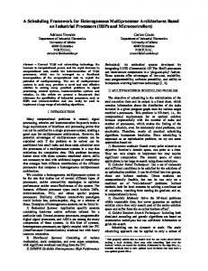
Figure 1. Representation of the function β(α), and the associated schedulability condition.

(≤ α) fit into each processor. Therefore, a multiprocessor made up of n processors can allocate at least βn tasks. Subsequently, if a task set is made up of m tasks and m ≤ βn, the task set is schedulable by RM and any reasonable allocation algorithm on n processors. By a reasonable allocation algorithm, we mean one which fails to allocate a task only when there is no processor in the system with enough remaining capacity to receive the task. Figure 1 depicts β as a function of α, and also shows the sufficient schedulability condition m ≤ βn. For example, if α is in the interval (21/3 − 1, 21/2 − 1] ≈ (0.26, 0414] then β = 2. In this case, the task set is schedulable if it has 2n tasks or less. Another consequence of the schedulability condition m ≤ βn is that it is worthwhile to obtain the value of the utilization bound only for the case m > βn. Otherwise, the task set is directly schedulable. From now we assume m > βn, so the above schedulability condition can not be applied. The rest of this section is devoted to the calculation of the utilization bound for RM scheduling and FF allocation, under the restriction m > βn. The strategy in the calculation is the following:

manuscript.tex; 25/10/2000; 18:27; p.7

8 1. Some mathematical relationships used in the proofs are presented. 2. Theorem 1 gives an upper limit on the utilization bound. 3. Lemma 3 is proved. This lemma is necessary in order to prove Theorem 2. 4. Theorem 2 proves an expression which relates the utilization bound for m tasks and n processors, with the utilization bound for (m−β) tasks and (n − 1) processors. 5. From the result given in step 4, and Liu & Layland’s bound for uniprocessors, Theorem 3 obtains a lower limit on the utilization bound. The upper and lower limits on the utilization bound given in steps 2 and 5 are the same. Finally, Theorem 3 gives the exact value of the utilization bound, which coincides with the upper and lower limits. RM-FF (m, n, α), some relationships of the positive Before calculating Uwc integer numbers, Z+, are presented without proof.

(i) x + 1 ≤ y

∀x, y ∈ Z+ | x < y

(ii) (21/x − 1)x > (21/y − 1)y > ln 2 ∀x, y ∈ Z+ | x < y (iii) (21/(x+1) − 1)x < (21/(y+1) − 1)y < ln 2

∀x, y ∈ Z+ | x < y

These will be referred to as Relationship (i), Relationship (ii), and Relationship (iii). The following theorem gives an upper limit on the utilization bound using RM scheduling and FF allocation. The proof is based on finding a task set which does not fit into the processors. THEOREM 1. If m > βn then RM-FF Uwc (m, n, α) ≤ (n − 1)(21/(β+1) − 1)β

+ (m − β(n − 1))(21/(m−β(n−1)) − 1)

(7)

Proof. Let us define g(m, n, α) = (n − 1)(21/(β+1) − 1)β + (m − β(n − 1))(21/(m−β(n−1)) − 1) We will prove that there exists a set of m tasks, {τ1 , . . . , τm }, with utilization factors 0 < ui ≤ α for all i = 1, . . . , m, and total utilization U = g(m, n, α) + ǫ, given ǫ → 0+ , which does not fit into n processors, using FF allocation and Liu & Layland’s bound for RM scheduling.

manuscript.tex; 25/10/2000; 18:27; p.8

9 This set of m tasks is made up of two subsets: a first subset with (m − βn) tasks, and a second subset with βn tasks. All the tasks of the first subset have the same utilization factor of value ui =

(m − β(n − 1))(21/(m−β(n−1)) − 1) − (21/(β+1) − 1)β (m − βn)

(8)

where i = 1, . . . , (m − βn). All the tasks of the second subset have the same utilization factor of value ǫ ui = (21/(β+1) − 1) + βn where i = (m − βn + 1), . . . , m. It can be easily checked that the total utilization of the whole task set is g(m, n, α) + ǫ. Firstly, it is necessary to prove that the utilization factors of both subsets are valid, i.e, 0 < ui ≤ α for all i = 1, . . . , m. Check of the utilization factors of the first subset. By hypothesis, m > βn, so m − β(n − 1) > β. Applying Relationship (i) we get m − β(n − 1) ≥ β + 1. Now applying Relationship (ii) makes (m − β(n − 1))(21/(m−β(n−1)) − 1) ≤ (β + 1)(21/(β+1) − 1). Considering this expression and equation (8) we get ui ≤

(21/(β+1) − 1) (m − βn)

(9)

On one hand, Lemma 2 provides the value β = ⌊1/ log2 (α + 1)⌋. Thus, (β + 1) > 1/ log2 (α + 1), and finding α α > (21/(β+1) − 1)

(10)

On the other hand m > βn by hypothesis, so (m − βn) > 0, and applying Relationship (i) we get m − βn ≥ 1

(11)

Substituting (10), and (11) into (9) proves that ui < α for all the tasks of the first subset. Next we will prove that all the utilization factors of the first subset are greater than zero. From Relationships (ii), (iii), and equation (11) we get (m − β(n − 1))(21/(m−β(n−1)) − 1) > ln 2 (21/(β+1) − 1)β < ln 2 m − βn ≥ 1

manuscript.tex; 25/10/2000; 18:27; p.9

10 Substituting the above expressions into equation (8) gives ui > 0 for all the tasks of the first subset. Check of the utilization factors of the second subset. It is always possible to find one real number between two real numbers. Hence, from equation (10), a positive value ǫ/(βn) must exist such that ǫ = ui (12) α > (21/(β+1) − 1) + βn which proves that the utilization factors of the second subset are less than α when ǫ → 0+ . In addition, the utilization factors of the second subset are obviously greater than zero. From the above results, we conclude that the proposed task set is valid. Next we prove that it does not fit into n processors, using Liu & Layland’s bound for RM scheduling and FF allocation. The first subset of tasks, {τ1 , . . . , τm−βn }, and the first β tasks of the second subset, {τm−βn+1 , . . . , τm−βn+β }, do not fit into processor P1 , since the total utilization of these tasks is over Liu & Layland’s bound. m−βn+β X

ui =

i=1

m−βn X i=1

ui +

m−βn+β X

ui

i=m−βn+1

= (m − β(n − 1))(21/(m−β(n−1)) − 1) +

ǫ n

> (m − β(n − 1))(21/(m−β(n−1)) − 1) However, from the above expression it can be proved that if task τm−βn+β is removed, then the first subset of tasks, and the first (β − 1) tasks of the second subset do fit into processor P1 . Hence, there are β(n−1)+1 tasks left of utilization factor, (21/(β+1) − ǫ , which FF tries to allocate to the last (n − 1) processors, 1) + βn {P2 , . . . , Pn }. No processor in the set {P2 , . . . , Pn } can allocate (β + 1) or more tasks of the second subset, since (β + 1) of these tasks together have a utilization over Liu & Layland’s bound. 

1/(β+1)

(β + 1) (2

ǫ − 1) + βn



> (β + 1)(21/(β+1) − 1)

However, each processor in {P2 , . . . , Pn } can allocate β tasks, as by the definition of β, at least β tasks can be allocated to each processor. Subsequently, tasks {τm−βn+β , . . . , τm−1 } are allocated to processors, but the last one, τm , can not be allocated to any processor.

manuscript.tex; 25/10/2000; 18:27; p.10

11 We conclude that the proposed task set of total utilization g(m, n, α)+ ǫ does not fit into n processors when ǫ → 0+ , so the utilization bound, RM-FF (m, n, α), must be less than or equal to g(m, n, α).  Uwc The proof of Theorem 2 requires Lemma 3, which is proved below. It relates the utilization bound for the same number of processors, but a different number of tasks. LEMMA 3. RM-FF RM-FF Uwc (q, n, α) ≥ Uwc (m, n, α)

for all q < m

Proof. This lemma will be proved by contradiction. Let us suppose that a pair of integers q and m exist, such that q < m, RM-FF (q, n, α) < U RM-FF (m, n, α). Between two real numbers, it and Uwc wc is always possible to find another real number, so we can find an ǫ > 0 such that RM-FF RM-FF RM-FF Uwc (q, n, α) < Uwc (m, n, α) − ǫ < Uwc (m, n, α)

By the definition of utilization bound, there exists at least one set of q tasks, {τ1 , . . . , τq }, of total utilization q X

RM-FF ui = Uwc (m, n, α) − ǫ

i=1

which does not fit into n processors. Next, we prove that this gives rise to a contradiction. If we add to this task set (m − q) new tasks, {τq+1 , . . . , τm }, each of utilization factor ǫ/(mP − q), we obtain a task set made up of m RM-FF (m, n, α), which fits into tasks of total utilization m i=1 ui = Uwc n processors. Hence, the first q tasks fit into n processors, which is a  contradiction. Next, we prove an expression which relates the utilization bound of multiprocessors with n and (n − 1) processors. This will allow us to obtain a lower limit for the utilization bound, going from the case n = 1 (uniprocessor case) to a general multiprocessor case with an arbitrary n. THEOREM 2. If m > βn then RM-FF RM-FF Uwc (m, n, α) ≥ (21/(β+1) − 1)β + Uwc (m − β, n − 1, α)

manuscript.tex; 25/10/2000; 18:27; p.11

12 RM-FF Uwc (m − β, n − 1, α) uk,1

τ1

···

u1 k−1 P

∆

τk−1

τk

τk+1

uk−1

uk

uk+1

···

um−β m P

ui

τm−β

···

τm um

ui

i=k

i=1

m−β P

ui

i=1

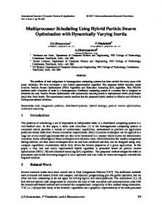
Figure 2. General situation in case 2 of Theorem 2.

Proof. We will prove that any set of m tasks {τ1 , . . . , τm }, with utilization factors 0 < ui ≤ α for all i = 1, . . . , m, and total utilization less than or equal to RM-FF (21/(β+1) − 1)β + Uwc (m − β, n − 1, α)

fits into n processors using Liu & Layland’s bound for RM scheduling and FF allocation. There are two possible cases: Case 1: The first (m − β) tasks have a total utilization less than RM-FF (m − β, n − 1, α), that is, Pm−β u ≤ U RM-FF (m − or equal to Uwc i wc i=1 β, n − 1, α). In this case the whole set of m tasks always fits into n processors, because the first (m − β) tasks fit into the first (n − 1) processors (since its utilization is below the bound), and the remaining β tasks fit into the last processor, since the definition of β implies that a least β tasks always fit into one processor. Case 2: The first (m − β) tasks have a total utilization greater than Pm−β RM-FF (m − β, n − 1, α). RM-FF (m − β, n − 1, α), that is, i=1 ui > Uwc Uwc In this case we will prove that the whole set of m tasks still fits into n RM-FF (m−β, n−1, α)+∆, processors if the total utilization is equal to Uwc 1/(β+1) provided ∆ ∈ R , and ∆ ≤ (2 − 1)β. A task τk must exist, whose uk added to the previous utilizations RM-FF (m − β, n − 1, α) to be exceeded. This ui , causes the bound Uwc situation is depicted in Figure 2, which is a graphical representation of the utilization factors of each task and the relationships between several quantities and summations used through this proof, for a generic set of m tasks in Case 2. It is important to observe that each rectangle in Figure 2 represents one of the m tasks making up the set, and the

manuscript.tex; 25/10/2000; 18:27; p.12

13 horizontal dimension of each rectangle gives the utilization factor of the task it represents. The value of k is obtained as the integer which fulfills: k−1 X

RM-FF ui ≤ Uwc (m − β, n − 1, α)
m − β we would be in case 1). It can be seen that the first (k − 1) tasks fit into the first (n − 1) processors. The total utilization of the first (k − 1) tasks fulfills k−1 X

RM-FF ui ≤ Uwc (m − β, n − 1, α)

i=1

Bearing in mind that k − 1 < m − β in Case 2, and applying Lemma 3, we get RM-FF RM-FF (k − 1, n − 1, α) Uwc (m − β, n − 1, α) ≤ Uwc

and thus

k−1 X

RM-FF ui ≤ Uwc (k − 1, n − 1, α)

i=1

Therefore, the first (k − 1) tasks fit into the first (n − 1) processors. We only have to prove that the remaining (m − k + 1) tasks fit into the last processor. The worst situation in terms of schedulability appears when all the tasks τi in {τk , . . . , τm } fulfill ui > uk,1 , where RM-FF uk,1 = Uwc (m − β, n − 1, α) −

k−1 X

ui

i=1

as shown in Figure 2. Note that if there were a task τi in {τk , . . . , τm } with ui ≤ uk,1 , we could always allocate this task to the first (n − 1) processors (since the addition of this new task does not cause the total utilization to exceed the bound), and the result would be a situation analogous to the current one, with k one unit greater. This reasoning can be repeated until no task τi with ui ≤ uk,1 exists among the last (m − k + 1) tasks, or until we are in Case 1. In order to prove that the last (m − k + 1) tasks fit into the last processor we have to prove that the total utilization of these tasks does not exceed Liu & Layland’s bound, that is, m X

ui ≤ (m − k + 1)(21/(m−k+1) − 1)

i=k

manuscript.tex; 25/10/2000; 18:27; p.13

14 Figure 2 shows that m X

ui = uk,1 + ∆

(13)

i=k

As already stated, all the utilization factors ui in this summation are greater than uk,1 , so (m − k + 1)uk,1 < uk,1 + ∆ < uk,1 + (21/(β+1) − 1)β by the definition of ∆. Finding uk,1 from the above equation uk,1