Validation of the Intensity-Based Source ... - GeoScienceWorld

Bulletin of the Seismological Society of America, Vol. 97, No. 5, pp. 1587–1606, October 2007, doi: 10.1785/0120060169

Validation of the Intensity-Based Source Inversions of Three Destructive California Earthquakes by Franco Pettenati and Livio Sirovich

Abstract The objective of our work is to invert the intensities of preinstrumental destructive earthquakes to retrieve their principal source characteristics. This is relevant in countries (as Italy and Greece) where a large and high-quality data bank of earthquake intensities during the past few centuries exists. We have previously validated our technique presented in this journal for the ML 5.9 1987 Whittier Narrows earthquake, and here we demonstrate that our algorithm works on three other earthquakes with known sources. Three more validations of the algorithm are presented here by using the site intensities observed by the U.S. Geological Survey for the M 6.4 1983 Coalinga, the MS 7.1 1989 Loma Prieta, and the Mw 6.7 1994 Northridge earthquakes. Our simplified KF formula simulates the body-wave radiation from a linear source, and 11 source parameters are retrieved: the three nucleation coordinates, the fault-plane solution, the seismic moment, the rupture velocities, the alongstrike and antistrike rupture lengths, and the shear-wave velocity in the half-space. To find the minima on the hypersurface of the residuals in the multiparameter model space, we use a genetic process with niching (Niching Genetic Algorithm) because we have already shown that the problem is bimodal for pure dip-slip mechanisms. The objective function of the nonlinear inversion is the sum of the squared residuals (calculated-minus-observed intensity at all sites). The three tests presented here were successful because the results agreed with the sources already known from instrumental measurements. A very accurate solution was found for Loma Prieta, notwithstanding the complexity of its source. In the two other cases, sources close to the reference ones were retrieved. The quality of our source determinations are obviously lower than those of instrumentally based models, but would be highly noteworthy for earthquakes without seismological recordings. The potential of the “KF inversions” seems particularly promising for European countries where seismicity rates are not very high, and where a lot of information on earthquake damage is available for preinstrumental earthquakes. The present series of validations raises our hope that further information on historic seismic events can be obtained from intensities, thus increasing the knowledge of seismotectonics and seismic hazard. Introduction Since the beginning of modern seismology, it has been hypothesized that the regional patterns of macroseismic intensity, I, data carry information about its source (e.g., Mallet, 1862; von Ko¨vesligethy, 1907; Jańosi, 1907; Blake, 1941; Sponheuer, 1960; Shebalin, 1973; Ohta and Satoh, 1980). I contains seismological information and is essential for the study of earthquakes of the preinstrumental era. Valuable results have recently been obtained after such data were analyzed with new, more quantitative techniques (e.g., Suhadolc et al., 1988; Zahradnik, 1989; Frankel, 1994; Johnston, 1996; Bakun and Wentworth, 1997; Wald et al., 1999; Gasperini, 2001; Shebalin, 2003; Molchan et al., 2004; Al-

barello and D’Amico, 2005). This kind of study seems especially promising for southern Europe, where a lot of documentation exists about seismic damage caused by old earthquakes. For example, Italy has an extraordinary data bank of high-quality macroseismic observations, obtained by seismologists and historians, who interpreted the reports written by the officers of the various kingdoms of the time, the gazettes, etc. The most complete data sets, referring to tens of destructive shocks, can be used for inversions back to the seventeenth century (as it has already been shown by Sirovich and Pettenati, 2001). The reader can examine the Italian intensity data on http://emidius.mi.ingv.it/DBMI04.

1587

1588 For example, there are promising data about destructive earthquakes in 1694, 1783, 1857, 1887, and 1920. Our new nonlinear intensity-based automatic inversion technique roughly identifies the principal geometric and kinematic characteristics of the causative sources of destructive earthquakes from their regional macroseismic intensity patterns (Gentile et al., 2004; Sirovich and Pettenati, 2004). We are aware that modern seismological techniques, which treat instrumental measurements, are able to give detailed pictures of the sources of earthquakes, but we are satisfied by approximate information because our strategic aim is to treat preinstrumental earthquakes. On the other hand, we could not treat too many source parameters because there was a risk of overparametrizing the inversion of intensities. First, we had to demonstrate that our algorithm works on earthquakes with known sources, and we did this for one recent earthquake, whose source was already well known from instrumental measurements, the 1987 ML 5.9 Whittier Narrows earthquake in southern California. The results retrieved from the analysis of its almost pure dip-slip mechanism fully validated both the grid-search inversion (Pettenati and Sirovich, 2003) and the genetic inversion (Gentile et al., 2004). Regarding the latter, we used a Genetic Algorithm (GA) with a population of 20,000 sources, and then a Niching Genetic Algorithm (NGA) with four demes of 2000 sources, obtaining almost the same couple of results (we are in a bimodal case). The most sensitive source parameters were the epicentral coordinates and the fault-plane solution. The two minimum variance models determined by both the GA and the NGA inversions were: (1) one east–west-trending dip-slip source, which is in agreement with that already known from instrumental measurements, and (2) one almost coinciding with its auxiliary plane in the fault-plane solution. For another test (a M 5.8–6.2 1936 earthquake in northeast Italy), we took the fault-plane solution, obtained independently from early P-wave readings, as our reference source (Sirovich and Pettenati, 2004). Similar studies, but on a more qualitative basis and without automatic inversion, had been conducted previously for the 1994 Northridge, the 1971 San Fernando, and the 1991 Sierra Madre earthquakes (Pettenati et al., 1999; Sirovich et al., 2001). We also attempted the inversion of one of the strongest events in the Mediterranean, which occurred in Sicily in seventeenth century (Sirovich and Pettenati, 2001); in this last case, we could only compare our results with seismotectonic interpretations from the literature. Our source for this seventeenth century event has been used already for the most recent official hazard maps of Italy by the Istituto Nazionale di Geofisica e Vulcanologia (see http://zonesismiche.mi.ingv.it/mappa_ ps_apr04/italia.html; last modified 29 October 2004). In this article we use the California modified Mercalli intensity (MMI) data obtained by the U.S. Geological Survey in the modified Mercalli scale of 1931 (Wood and Neumann, 1931) to validate our technique more thoroughly. Note that what we call “pseudointensity” (in arabic numbers) refers to both the intensity calculated by our

F. Pettenati and L. Sirovich

model, stated as an integer number, and the intensity observed in the field when described with a cartesian axis. This is done to observe the definition of I (a discrete and bounded scale that increases monotonically with unequal steps) (Barosh, 1969; Musson et al., 2006). In this article, all figures showing the results of the intensity surveys and our synthetic patterns of pseudointensity were produced by our natural-neighbor bivariate interpolation scheme “n-n” of 2002, which is based on the Voronoi tessellation (Sirovich et al., 2002). Recently, we implemented a new analytical algorithm, which gives the same results but is much faster and solves some interpolation problems on the borders of the sampled area, where the Voronoi polygons diverge. We remind that the n-n isolines shown in the following figures are determined in a unique way; the n-n algorithm is deterministic, it has no adjustable parameters at all, and it has an all-pass filter nature. In other words, it strictly honors the data, and the isolines are obtained without any explicit or implicit assumption about the observed phenomenon. Thus, everybody obtains the same result. To draw the following n-n isoseismals, we used all data sites within a 0.1⬚-wide strip around the shown areas. Then, we inverted only the data inside the shown areas. The Model Used For the radiation model used in this article, we use the KF formula that has previously been presented (Sirovich, 1996, 1997; Pettenati et al., 1999; Sirovich and Pettenati, 2001, 2004). KF considers the body-wave radiation from a line source in an elastic half-space in the distance range of approximately 10 to 100 km from the source. It uses 11 parameters: the hypocentral latitude and longitude, the faultplane solution (strike, dip, and rake angle), the seismic moment M0, the depth of the line source H (equal to the nucleation depth), the shear-wave velocity VS, the rupture velocities Vr along-strike and antistrike, the along-strike percentage of the total rupture length L. L comes from M0, through the empirical relationship by Wells and Coppersmith (1994; p. 990, Table 2A; “Slip type” ⳱ “All,” “subsurface rupture length”). The antistrike rupture length is obtained as the difference. The KF formula agrees with the asymptotic approximation (Spudich and Frazer, 1984; Madariaga and Bernard, 1985), assuming that the seismic source is a dislocation propagating horizontally on a rupture plane of unit width. In this approach, only the highfrequency radiation from the source is considered (where high frequency means wavelengths shorter than the shortest observer–source distance). Note that it has been repeatedly proved that the high-frequency approximation works satisfactorily even at distances of the order of the wavelength (e.g., Bernard and Madariaga, 1984; Spudich and Frazer, 1984; Madariaga and Bernard, 1985). In the present study, we chose to stay under the 80-km distance, and no adjustments of the study areas were done. However, for Northridge, we chose the same area that had

Validation of the Intensity-Based Source Inversions of Three Destructive California Earthquakes

been taken into account in our previous study (approximately 60 km epicentral distance in Sirovich, 1996, figure 6), so that the two results are mutually comparable. In these cases, there were three sites closer than 5 km to the projection of the source segment. Because the asymptotic approximation does not hold here, the sites received the maximum pseudointensity value calculated at the site closest to the source, but outside the 5-km limit. Given the half-space model, the nucleation depth we retrieve is not well resolved. Our graphical convention is that the fault plane dips to the right of the positive direction of the strike, which ranges between 0⬚ and 360⬚, and the rake angle is seen on the fault plane from the hanging wall of the fault, and measured counterclockwise from 0⬚ to 360⬚ between the positive direction of the strike and the direction of the slip vector. Our source model has unit width and, thus, in prior work we have shown the sources we retrieved as segments. However, in this article we draw the source obtained from inversion as a plane projected on the Earth’s surface; its width again obtained from Wells and Coppersmith (1994; empirical relationship number 4, p. 990, Table 2A; “Slip type” ⳱ “All”) from the seismic moment, M0, by the relation mentioned by Wells and Coppersmith, via the empirical relation M 2/3(log M0) ⳮ 10.7 by Hanks and Kanamori (1979), where M is the moment magnitude. Then, we also show the virtual intersection between the prolongation of the theoretical rupture plane and the earth’s surface. We do this for potential seismotectonic purposes and also to follow what is currently being done in Italy by the May 2005 release of the Database of Individual Seismogenic Sources (version 3) of the Istituto Nazionale di Geofisica e Vulcanologia of Italy (http://www.ingv.it/%7ewwwpaleo/DISS3/). To calculate the pseudointensity at a site from the KF value there, we used an empirical correlation obtained from 1720 observations from five earthquakes in the Greater Los Angeles Region (see paragraph 2 by Sirovich et al., 2001; and equation 2 by Pettenati and Sirovich, 2003). The values of pseudointensities were rounded to give integers. We should also bear in mind two intrinsic limitations of our KF procedure. First, we are unable to discriminate between the results produced by mechanisms that differ by 180⬚ in the rake angle. This is because, in both cases, it produces the same radiation but with reversed polarities (this ambiguity may be solved only with additional tectonic/geodynamic information). For this reason, in this article we chose to draw the beach balls of the fault-plane solutions we obtained from inversion without colors. Second, in the almost pure dip-slip mechanisms, our KF inversion problem is close to bimodality (Gentile et al., 2004). Thus, we use a sharing NGA inversion technique (Martin et al., 1992). The Nonlinear Inversion of Intensity We searched for the absolute minimum variance model in the 11-source parameter model space by employing a sharing NGA. For NGA, we adopted some routines from the

1589

Figure 1.

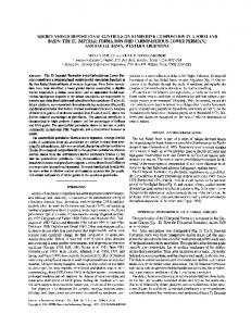
Coalinga 1983 earthquake. Tessellated observed intensities (black dots, National Geophysical Data Center, see text). The arrow points to the approximate area of the main shock cluster of aftershocks (after Fehler and Johnson, 1989). The Pacific Ocean shore is in the lower left corner.

Parallel Genetic Algorithm Library by Levine (1996) and used four separate subpopulations of individuals (i.e., sources). Each subpopulation had 500 sources and evolved independently from the others. According to the genetic similarity, each source individual is characterized by a string of 11 unknown source parameters (genes). In this approach, within every generation, one selection and three evolutionary (stochastic) steps are applied: first, the best individuals (90% of the source models) are chosen in the selection step; second, they are “married” in the crossover step (with 90% fertility); third, in the mutation step, the 6% of the new 500 individuals (450 “sons” plus 50 nonfertile parents) receive a new value for one parameter by chance; fourth, crowding deletes identical individuals and prevents each subpopulation from quickly converging to a false minimum. The genetic process is allowed to go on for N generations. This ensures that the virtual space of the parameters is properly explored. In particular, in the evolution logic, we chose to always have the best source of each generation transmitted to the new generation. NGA also involves the sharing step, which allows subpopulations of sources to survive within parameter subspaces (niches), so that each source of each subpopulation is not in competition with the sources of other subpopulations living in other niches. Each subpopulation of sources evolves independently from the others because, in this step, the normalized distance between each source of a subpopulation and each source of all the other subpopulations obeys a certain condition (equation 1 by Koper et al., 1999). Since our NGA inversion technique has already been

1590


presented (Gentile et al., 2004; Sirovich and Pettenati, 2004), we refer the reader to the aforementioned articles for details. Regarding the resolution of our inversion results, they correspond to the incremental variations shown in Table 1. Table 1 also shows the ranges explored. As seen here, no constraints were adopted for the fault-plane solution and for the nucleation location (some limits are obvious in the latter case), and wide ranges were chosen for the other parameters. The objective function during inversion was Rrs2, where rs is the pseudointensity calculated at a site, minus the intensity observed there (the suffix denotes the sites). We looked for the source models that minimized the sum of the squared residuals of intensities, that is, those that had the best fitness. For validation purposes, we related mostly to instrumental and modeling results produced relatively soon after each event. We did this for two reasons: (1) because we wanted to see if it was possible to get an approximate idea of the sources by using the intensities, we did not need the detailed results recently obtained by advanced instrumental techniques; (2) for conciseness. Finally, from a more general point of view, we are aware that the results obtained by authors who used instrumental measurements are much more reliable than ours. But, to repeat, we decided to rely on the felt intensities because we wanted to explore whether it is possible to get an approximate idea of the sources of preinstrumental earthquakes by using these semiquantitative data. We proved that this is feasible using automatic genetic inversions.

The Inversion Errors No intensity estimates from several independent researchers were available for the study cases, and thus, it has been impossible to calculate the inversion errors in a physically meaningful way. For this reason, in the present article, we have the recourse of two strategies for data randomization: (1) Monte Carlo and (2) the approach we have followed in previous articles. In the first case, for each source parameter, we created a random number N of artificial intensity data sets, with 50 ⬍ N ⬍ 250. Next, we assigned new intensity values to all sites, and each artificial set complied with the following conditions. The artificial values had to lie within the I–XI limits. Starting from a normal distribution with zero as the mean and one degree of variance, the maximum difference between the artificial value and the observed intensity was two degrees. However, we made one exception: we reasoned that the limit between the V and the VI degrees (i.e., between nondamage and damage) is particularly reliable, and thus decided that the intensities ⱕV cannot exceed the VI value, and those ⱖVI cannot go under the V value. In so doing, an average of 23–25% of the observed intensities were substituted for the three earthquakes studied. For the latter randomization, we followed exactly the

Table 1 Space of the Source Parameters Parameter

Incremental Variation

Explored Range

Strike angle (⬚) Dip angle (⬚) Rake angle (⬚) Ⳳ 180⬚ Nucleation longitude (⬚) Nucleation latitude (⬚) Nucleation depth H (km) VS (km/sec) Mach number (Vr /VS) M0 (1018 N m)

1 1 1 0.01 0.01 0.1 0.01 0.01 0.01

0–359 0–90 0–180 Ⳳ0.40 Ⳳ0.35 5.0–27.0 3.40–3.95 0.50–0.99 see the individual case

procedure we adopted in our previous articles, starting from Pettenati and Sirovich (2003). N was chosen between 50 and 200, a fixed 37% of the original data was replaced by artificial substitutes, which followed a normal distribution (thus, the maximum intensity change at a few sites reached four degrees, over the total of 9,300–37,200 synthetic data points for each source parameter). The I–XI limit and the other conditions of case (1) were obeyed. It is worth mentioning that in previous articles (Pettenati and Sirovich, 2003; Gentile et al., 2004; Sirovich and Pettenati, 2004), we referred to our randomization (2) as being the bootstrap technique of Numerical Recipes (Press et al., 1992, pp. 684–687); but we realized that this was an erroneous statement. In the tables showing our inversion results, we show that both kinds of errors (1) and (2) allow the comparison. To calculate them, we inverted each synthetic intensity data set and obtained S values for the source parameter. Each inversion complied with the following conditions: (1) the range of the explored space of the parameter is equal to the range explored to find the minimum variance model; (2) the parameter belonging to the minimum variance model stands at the center of this range. Subsequently, we calculated the standard deviation of each source parameter by analyzing the SⳭ1 parameters obtained (from the S inversions, plus the parameter of the minimum variance model), and took two standard deviations as the 95% probability errors. This held for both randomizations (1) and (2).

Statistical Outliers Before performing the inversions, one has to search for statistical outliers that could be errors, unexplained anomalies, or even strong site effects. For this, we applied the classical Chauvenet method (Barnett and Lewis, 1978, p. 19– 20; see also Johnston, 1996) to the epicentral distances d(I). Let us recall that the Chauvenet method assumes that d(I) follows a log-normal distribution. This holds for the Northridge data set, where we found four statistical outliers: Los Nietos, Glendora, Bullhead City, and Reseda. We did not use these data in the inversion and they are not shown in the figures. For the case of Reseda, see the Discussion. The Coalinga data set had no outliers.


The log-normal distribution does not hold well for the Loma Prieta earthquake. Therefore, we kept the only one outlier, Alviso, for our geotechnical and statistical uncertainty (see the Discussion).

Site Effects In general, grouped site effects would obviously bias the inversion; isolated site effects increase the noise of the inversion but are not expected to condition the results heavily. An objective criterion for evaluation of all the sites is required, however. Otherwise, if only certain site values are corrected, we risk being criticized for having examined only selected data or for having modified those data to drive the inversions toward our desired results. Stating that we did these corrections on the basis of specific studies on individual sites, carried out by other authors, would not be enough. For example, in the case of the Northridge 1994 earthquake, we were aware of the focusing effects in North Hollywood and in Santa Monica (e.g., Gao et al., 1996; Baher et al., 2002). The first area experienced the degree VIII at North Hollywood (Lank.) and the IX at Sherman Oaks. Then, there were two degrees VIII and one degree IX (the St. Johns Hospital site) in the Santa Monica area. A one degree amplification could be easily hypothesized in the five cases, but the reassigned values would not change the shape of the large area of VIII degree southeast of the epicenter (see Fig. 7a). From a statistical point of view, the three d(I⳱VIII) values are fully compatible with the d(I⳱VII)

1591

distribution, and the d(I⳱IX) of St. Johns Hospital and Sherman Oaks are fully compatible with the d(I⳱VIII) distribution. In light of this situation, we kept the original data. To strenghten our choice of avoiding personalized corrections, we mention that: (1) deamplifications, if any, usually do not catch the attention of the researchers as the cases of amplification do, but have the same importance as far as inversion is concerned; (2) detailed and specific studies were available only for a very limited number of sites. A similar situation holds for the Loma Prieta 1989 shock. Here, for example, we were aware that the Alviso site most likely experienced deamplification (degree V at less than 45 km), but no specific studies were available (see the Discussion). Incidentally, we have also considered that, because of the lack of geophysical data, we could not compute the empirical correction factors for the intensities as obtained by Hruby and Beresnev (2003) for the strong-motion spectra in the Los Angeles Basin. Thus, we performed d(I) regressions as in Pettenati and Sirovich (2003; p. 50 and Fig. 3) and also made an attempt to consider the NEHRP VS30 classification (see the Discussion). The site geology was tentatively taken into account by splitting the epicentral distances of the sites, d(I), by the three following lithologic classes (R.M.S. Inc.; Fouad Bendimerad, 1997, written comm.). Class 1 (Rock). Hard to firm rock, mostly metamorphic and igneous, fresh conglomerates, sandstones and shales without intensive fracturing. VS in general ⬎700 m/sec.

Figure 2. Coalinga 1983 earthquake. Black dots as in Figure 1. Intensities were interpolated by the n-n algorithm (Sirovich et al., 2002). (a) Observed intensities as in Figure 1. (b) Synthetic pseudointensities produced by the minimum variance model 4 of Table 3 (also see its beach ball in the figure); the bilateral source retrieved by inversion is in black (see its details in the inlet); its nucleation is in the center of the white error cross.

1592


Class 2 (Weak Rock/Stiff Soil). Gravelly soils to weak rock. Deeply weathered and highly fractured bedrock. Soils with more than 20% gravel. Alluvial cover less than 5 to 10 m thick and not water-saturated. VS 375–700 m/sec. Class 3 (Soft Soil). Stiff clay and sandy soils. Loose to dense sands, silty or sandy loams, and medium to stiff/hard clays. Water-saturated alluvial deposits. Holocene alluvium ⬎10 m thick. VS 200–375 m/sec.

The Treated Cases The Coalinga M 6.4 1983 Earthquake Table 2 summarizes the ranges of the reference source parameters of the 1983 Coalinga earthquake, which were obtained from instrumental measurements by different authors, independent from this study. For brevity, only the ranges of the values (errors included) from a selection of the available bibliography are reported. Figure 1 shows the site intensities used for the present study. They come from the National Geophysical Data Center (NGDC) (see http://www.ngdc.noaa.gov/seg/hazard/ earthqk.shtml) and are in the MMI scale. The surveyed sites are shown as black dots, the intensities were tessellated by Voronoi polygons (Pettenati et al., 1999; Okabe et al., 2000). In the figure, we also show the mainshock cluster of aftershocks reported by Fehler and Johnson (1989; Fig. 1a). Note that in the legend, we use Roman numerals for the intensities observed in the field. In Figure 2a, the same intensities were contoured with our n-n isoseismals, which use the aforementioned naturalneighbor interpolation principle (Sirovich et al., 2002). Here, we also show: (1) as a star, an early epicenter by Stein and King (1984), and, as a circle, an epicenter by Ellsworth

Table 2 Source Parameters of the Coalinga 1983 Earthquake Obtained from Instrumental Measurements by Different Authors From Instrumental Measurements

Strike angle (⬚) Dip angle (⬚) Rake angle (⬚) Nucleation longitude (⬚) Nucleation latitude (⬚) Nucleation depth H (km) Rupture length L (km) VS (km/sec) MachⳭ Machⳮ M0 (1018 N m)

Figure 3. Site effects in the three data sets. Rocky and stiff sites are marked by “1–2,” soft sites by “3.” The rectangles DIr include the distance and intensity ranges of the sites shown in Figures 2a, 6a, and 7a, respectively. Regression lines and 95% confidence bands. (a) 1983 Coalinga. (b) 1989 Loma Prieta. (c) 1994 Northridge.

Value

294–319*† 60–88*† 71–97*†‡ ⳮ120.29–ⳮ120.34§ 36.19–36.23§ 4.7–12㛳 13.4–35# 0.75** 0.75** 5.04††

*Data from: Stein, 1983; Stein and King, 1984; Sipkin, 1986; Fehler and Johnson, 1989; Choy, 1990; Eaton, 1990; Sipkin and Needham, 1990. At the beginning, some authors accredited the southwest-dipping auxiliary plane. The fault-plane mechanism of the latter subevent by Choy (1990; strike ⳱ 300 Ⳳ 5⬚, dip ⳱ 80 Ⳳ 5⬚, rake ⳱ 80 Ⳳ 15⬚) is a bit outside the shown range. † Mavko et al. (1985) proposed: strike angle ⳱ 300–315⬚, dip ⳱ 60– 75⬚, and rake ⳱ 90⬚. ‡ Sipkin and Needham (1990) gave major credit to the value of 90⬚, “but the data do not preclude rakes from 60⬚ to 120⬚”; the three-point technique by Fehler and Johnson (1989) does not determine the rake angle. § Stein and King, 1984; Ellsworth, 1990. 㛳 Stein and King, 1984; Sipkin, 1986; Choy, 1990; Sipkin and Needham, 1990. # 13.4–29.4 km, cumulative from the two subevents by Choy (1990), errors included. From the aftershock distribution: 35 km (Stein, 1983), 25 km (Wesnousky, 1986). **Choy, 1990. †† Cosmos Virtual Data Center (http://db.cosmos-eq.org/).


1593

Figure 4.

Example of exploration of the model space of the parameters of the faultplane solution of the 1983 Coalinga earthquake by calculating the squared pseudointensity residuals 兺rs2 at the surveyed sites. The cross shows the 兺rs2 ⳱ 40 very small area, where the minimum variance model 4 of Table 3, with 兺rs2 ⳱ 36, was found. Abscissas, strike angles from 0⬚ to 359⬚; ordinates, rake angles from 0⬚ to 179⬚.

(1990); (2) an example of the reference fault-plane solutions, which are summarized in Table 2 (the one shown from the first P-wave pulses uses the central values proposed by Mavko et al. [1985] listed in the note † of Table 2); and (3) as a rectangle, an example of the reference rupture planes summarized in Table 2, that is, that found by Stein and King (1984) by modeling geodetic data by uniform slip on a rectangular plane, with dislocations embedded in an elastic halfspace. Note that the n-n ⱖV isoseismals of Figure 2a are not very different from the isoseismals hand-drawn by Stover and Coffman (1993; Fig. 23). This confirms that the use of

the natural-neighbor principle could match the best American practice, as was noticed in the isoseismals of the 1994 Northridge earthquake hand-traced by Dewey et al. (1995, Fig. 2; Sirovich et al., 2002, pp. 1936–1937). The n-n isoseismals define isolated local positive and negative “anomalies,” as in Figure 2a. From the seismological point of view, they are of unknown origin. However, they strictly obey the information territorial density and continuity shown by the tesserac of Figure 1. Note that traditional hand-drawn isoseismals would have connected those data, or left them as isolated anomalies, arbitrarily. What is most relevant for the

1594


present inversions is that Figures 1 and 2a show that: (1) there are few sampled sites in the northwest and southeast directions from the center of the figures; (2) there is only one site of degree VII; (3) the sites of degree V are approximately isotropically distributed around the maximum intensities, whereas the 15 sites with degree IV are concentrated in the four corners of Figures 1 and 2a. As will be seen later, this situation constrains what results are obtainable. Figure 3a shows the search for site effects in the 1983 Coalinga data set. The examined set contains sites with soil classification data (Sirovich et al., 2001) and intensity observations from the NGDC data set. We were obliged to omit intensities II, VII, and VIII because of scarcity of data. Thus, 214 III to VI data were used. The regression analyses were performed with a commercial package (StatView, version 4.51); the data points and the 95% confidence intervals are shown. The rocky and stiff sites (categories 1 and 2, 67 data; see the continuous curves) were grouped together for geotechnical and statistical considerations. Regression 3 in Figure 3a (dashed curves and dark gray confidence interval) refers to 147 sites with soft soils. We also patterned in light gray the rectangle (Dir) of the distance and intensity range of the sites shown in Figure 2a. In the figure, soft soils (3) seem to deamplify at short distances and to amplify at long distances, but the confidence bands overlap all over the considered ranges. Thus, we concluded that this observation is not statistically reliable, even if it is physically plausible. We therefore neglected site effects in the inversion process. Consider, however, that below 100 km the maximum intensity difference between regression lines (3) and (1–2) in Figure 3a would be approximately half an intensity degree (also see the later cases and the Discussion). Table 3 presents the minimum variance source models found by the subpopulations 4, 1, and 3 of our NGA inversion of the Coalinga 1983 earthquake. Model 4 corresponds to the hypothesized rupture plane (see later). Model 2 is not shown because it is much worse than the others (Rrs2 54, longitude ⳮ113.63⬚, latitude 36.12⬚, dip 59⬚, rake 176⬚). As has been established, in the table in parentheses, we first show the inversion errors calculated by the Monte Carlo method and, second, those obtained using a previous approach (Pettenati and Sirovich, 2003).

Figure 5.

As in Figure 4, but searching over the epicentral coordinates of the 1983 Coalinga earthquake, and for the strike angle of the rupture plane (from 310⬚ to 330⬚ in the figure). The cross shows the 兺rs2 ⳱ 40 area, where the minimum variance model 4 of Table 3 was found. Abscissas: epicentral longitude; ordinates: epicentral latitude.

The Hypersurface of the Residuals. In Figure 4, we show the final stage of the automatic exploration of the whole space of 兺rs2. The source with the minimum 兺rs2 (model 4) is in the cross center (dip ⳱ 87⬚, 兺rs2 ⳱ 36. For graphical reasons, the figure is in three dimensions (strike, dip, rake of the fault-plane solution); regarding the other parameters, the three panels use those of model 4 listed in Table 3. The scale is in the figure; the highest residuals 240 ⬍ 兺rs2 ⱕ 320 and 320 ⬍ 兺rs2 ⱕ 400 were shown with only two gray densities, and the relatively large residual peaks, with 兺rs2 ⬎ 400, were shown in white. The small white area in the cross center corresponds to 兺rs2 ⱕ 40 . Model 4 of Table 3 is the hypothesized rupture plane. Note that in Figure 4,

1595


Table 3 Source Parameters of the Minimum Variance Source Models Found by the NGA Inversion for the Coalinga 1983 Earthquake NGA Inversion (97 Data)

Parameter

Strike angle (⬚) Dip angle (⬚) Rake angle* (⬚) Nucleation longitude (⬚) Nucleation latitude (⬚) Nucleation depth H (km) Rupture length L† (km) VS (km/sec) MachⳭ† Machⳮ† M0 (1018 N m) Rrs2

Model 4 (Rupture Plane) (Subpopulation 4) Value Ⳳ error

320 (Ⳳ15; Ⳳ24) 87 (Ⳳ8; Ⳳ10) 73 (Ⳳ10; Ⳳ10) ⳮ120.34 (Ⳳ0.20; Ⳳ0.22) 36.19 (Ⳳ0.22; Ⳳ0.12) 21.3 (Ⳳ7; Ⳳ5.7) Lⳮ ⳱ 17.8; LⳭ ⳱ 4.5 3.94 (Ⳳ0.13; Ⳳ0.18) 0.69 (Ⳳ0.12; Ⳳ0.12) 0.91 (Ⳳ0.09; Ⳳ0.10) 5.04 (Ⳳ4.80; Ⳳ4.60) 36

Model 1 (Subpopulation 1) Value


256

98

40

90

117

114

ⳮ120.48

ⳮ120.43

36.14

36.18

21.5

22.0

Lⳮ ⳱ 15.0; LⳭ ⳱ 7.7 3.55

Lⳮ ⳱ 3.3; LⳭ ⳱ 20.4 3.72

0.66

0.86

0.70

0.60

5.26

5.88

38

39

*With an ambiguity of Ⳳ180⬚, see text. † Positive along-strike, negative antistrike; the error of the total length is Ⳳ9.0 km.

we show the whole ranges of the strike and rake angles, with a 1⬚ step, and the 77–87⬚ range for the dip angle, with a 5⬚ step. The last limitation is for graphical purposes, although the whole excursion of the dip angle was explored with a 1⬚ step. Figure 5 shows the final exploration of the model space of 兺rs2 in the 3D parameter space of the two epicentral coordinates and the strike angle. Only the topographies given by the strike angle equal to 310⬚, 320⬚, and 330⬚ are shown. The central sketch, for 320⬚ strike, corresponds to the bestfitting model 4 in Table 3 (inside the open cross in the figure). In the cases that we studied previously (Pettenati and Sirovich, 2003; Gentile et al., 2004; Sirovich and Pettenati, 2004), the structure of 兺rs2 constrained the epicenters very well, because they fell inside deep and approximately circular depressions. However, the peculiar structure of the subfigures in Figure 5 constrains the result more weakly than in the aforementioned cases. The principal depression (black, 兺rs2 ⱕ 60 is oriented northwest-southeast, like the orientation of the unsampled epicentral area in Figures 1 and 2a. Nevertheless, the deepest minimum, corresponding to the best-fitting 320⬚ strike angle, lies inside a pronounced depression. Finally, 兺rs2 is rather sensitive to the strike angle. Validation of the Inversion.

Starting from what we have

just seen in Figure 5, the epicentral coordinates of model 4 of Table 3 match well to the reference values of Table 2. However, the figure demonstrates that the peculiar geographical sampling of the Coalinga intensities is unable to constrain the epicenter strongly, as is usual in our albeit limited experience. In general, the central values of the source parameters of model 4 in Table 3 are inside the ranges shown in Table 2, or very close to them. There are some minor exceptions, however. First, our nucleation depth is too large (but, as we already stated, this may be due to the simple velocity structure). Then, we lack a sufficient set of reference values both for VS and the Mach number (⳱Vr /VS) (apart from the proposal by Choy, 1990, in Table 2), but our VS in the half-space seems too high. Finally, our Mach numbers are scattered around the reference values, but perhaps this is not dramatic in light of the data that we treat and the strategic target of our work. In conclusion, we are confident that model 4 is sufficiently validated. In particular, the faultplane solution, the epicentral coordinates, and the dimension of the source were well retrieved. Then, by comparing Tables 2 and 3, it can be easily seen that models 1 and 3 are not validated. Finally, Figure 2b shows the n-n isoseismals of the synthetic pseudointensities (in arabic numbers) produced by the minimum variance model 4 of Table 3, calculated at the

1596


Figure 6. 1989 Loma Prieta earthquake. Interpolation as in Figure 2. (a) Intensities observed by the U.S. Geological Survey in the black dots (courtesy of J. W. Dewey, written comm., 2003); the white star and the white rectangle are the epicenter and the projection of the source by Wald et al. (1991); the white dotted curve is the isoseismal of VIII degree according to Stover et al. (1990); the upper fault-plane solution is by both Oppenheimer (1990) and Choy and Boatwright (1990), see the text for the lower one for the southeastern fault segment. (b) Nucleation, projection of the bilateral source and its virtual intersection with the topographical surface, fault-plane solution, and synthetic isoseismals of the minimum variance model 4 of Table 5.

Figure 7. 1994 Northridge earthquake. (a) Intensities observed by the U.S. Geological Survey in the black dots; for the two white rectangles see the text. (b) Nucleation, projection of the bilateral source and its virtual intersection with the topographical surface, fault-plane solution, and synthetic isoseismals of the minimum variance model 1 of Table 7.

1597


sparse sites. Figure 2b also shows the source obtained by Stein and King (1984) and the mainshock cluster (repeated from Fig. 1) along with: (1) our fault-plane solution (without colors, as mentioned earlier); (2) the projection of the line source retrieved by the regional pattern of intensity (in black), with (3) our epicentral error (see the white cross with bars, in this case at one standard deviation). Due to the dip of the source plane shown (87⬚; Table 3), its projected width, its virtual intersection with the Earth’s surface, and the nucleation location can be graphically resolved only in the closeup in the upper left corner of the figure. Our projected source plane compares well with that by Stein and King (1984). Regarding the synthetic pseudointensity field in Fig. 2b, note that: (1) the model obtained by automatic inversion is able to reproduce the three maximum intensities of degrees VII and VIII in the meizoseismal area in Figure 2a; (2) the extensions of the areas of the synthetic isoseismals approximately match the ones of Figure 2. Regarding some shapes, which do not match well, let us recall that they are shown for the reader’s convenience, but in the sparsely sampled epicentral area they are unreliable.

The Loma Prieta MS 7.1 1989 Earthquake Table 4 shows the same kind of reference data as in Table 2, but for the 1989 Loma Prieta earthquake. The parameters shown refer to the initial rupture, which had a pronounced oblique slip. Figure 6a shows the n-n isoseismals obtained from the U.S. Geological Survey site intensities (black dots, courtesy of J. W. Dewey, written comm., 2003). For brevity, we omit the figure of the Voronoi polygons. The I data from the San Francisco Bay area were omitted from Figure 6a because of the aforementioned limitation in the distance range where we can use the KF formula for body waves. This however allowed us to omit a series of data of VII, VIII, and even IX degree (five sites related to the Marina District tragedy) in downtown San Francisco, which were clearly “anomalous” and would have biased our inversion. Instead, we kept the aforementioned Alviso site. Note that if it is disregarded in Figure 6a, the match with Figure 6b improves. Thus, this choice was on the side of caution. Then, notwithstanding the presence of the ocean, some elongation of the isoseismal of VIII degree in the northwest–southeast direction could be tentatively inferred from Figure 6a. Also note the area of degree V in the northeast corner. Then, the figure shows: (1) the epicenter (see the star) and the projection of the fault representative of that found by various authors (the ones shown are from Wald et al., 1991); (2) the early fault-plane solution proposed by both Oppenheimer (1990) and Choy and Boatwright (1990) for the initial rupture (see the upper beach ball in the figure); and (3) an example of the almost pure strike-slip mechanism proposed by various authors for the southern part of the fault. The one shown in the lower beach ball in Figure 6a rounds the rake by Beroza (1991)

Table 4 Source Parameters of the Loma Prieta 1989 Earthquake Obtained from Instrumental Measurements by Different Authors Value From Instrumental Measurements

Strike angle (⬚) Dip angle (⬚) Rake angle (⬚) Nucleation longitude (⬚) Nucleation latitude (⬚) Nucleation depth H (km) Rupture length L (km) VS (km/sec) MachⳭ Machⳮ M0 [1019 N m]

From Seismological Measurements

From Geodetic Measurements*

117–144† 53–85† 110–158†‡ ⳮ121.88㛳 37.04㛳 10–25# 30–40†† 3.7§§ 0.75–0.80㛳㛳 0.75–0.80㛳㛳 1.3–3.9##

126–129 57–60 139–163§ ⳮ122.023–ⳮ122.003 37.153–37.167 12** 32–44‡‡

2.6–3.0

*Marshall et al. (1991; see their “acceptable ranges for a planar fault” in their Table 6). † Langston et al. (1990); Oppenheimer (1990); Kanamori and Satake (1990); Choy and Boatwright (1990); Ruff and Tichelaar (1990); Plafker and Galloway (1989); Dietz and Ellsworth (1990), who do not propose a rake angle, however; for the values retrieved by Wald et al. (1991), see the Discussion. ‡ Various authors find almost pure strike-slip mechanism in the southern half of the fault (e.g., rake ⬃160–170⬚, Beroza, 1991; Steidl et al., 1991). § The upper limit is from Lisowski et al. (1990). 㛳 Dietz and Ellsworth (1990); Ruff and Tichelaar (1990). # Plafker and Galloway (1989); Dietz and Ellsworth (1990); Oppenheimer (1990); Choy and Boatwright (1990); Ruff and Tichelaar (1990); Wallace et al. (1991); Romanawicz and Lyon-Caen (1990). **From Marshall et al. (1991; see their section CC⬘ in Fig. 10 for an elastic half-space). †† Dietz and Ellsworth (1990); Kanamori and Satake (1990); Ruff and Tichelaar (1990); Wald et al. (1991); all authors suggest a bilateral rupture. ‡‡ The upper values are by Lisowski et al. (1996) and Wu and Rudnicki (1996). §§ Choy and Boatwright (1990); Ruff and Tichelaar (1990). 㛳㛳 Choy and Boatwright (1990); Beroza (1991); Hartzell et al. (1991) suggest Vr ⳱ 2.5 km/sec. ## Kanamori and Satake (1990); Choy and Boatwright (1990); Ruff and Tichelaar (1990); Barker and Salzberg (1990); Na´beˆlek (1990); Romanawicz and Lyon-Caen (1990); Zhang and Lay (1990); Beroza (1991).

and Steidl et al. (1991) (approximately 160–170⬚; also see Wald et al. [1991] and Table 4). Figure 3b shows the same kind of search for site effects as in Figure 3a. In this case, 234 sites had intensity data and site classifications. The grouping of sites (158 soft sites in class 3; 76 rocky and stiff sites in classes 1–2), the regressions, the confidence intervals, and the graphical convention are also as in Figure 3a, but the range is from intensity III to VIII. From the figure, it is seen that no statistically significant difference exists between groups 3 and 1–2, not at all within our inversion range (refer to the rectangle DIr, patterned in light gray, in Fig. 3b. See also Fig. 6a). With respect to the inversion in this case, we realized that the depression of the Rrs2 residuals in the hypersurface of the 11-parameter model space was rather flat around the

1598


absolute minimum. Nevertheless, the structure of 兺rs2 in the virtual three-parameter space of the epicentral coordinates and of the strike angle was well defined and almost concentric (as was the case of our previous inversion of the Whittier Narrows 1987 earthquake; see Figs. 7 and 11 in Pettenati and Sirovich, 2003). For brevity, we omit the explorations of the model space as we showed in the Coalinga case (Figs. 4 and 5). Thus, we used six subpopulations to explore the 11-parameter model hyperspace and found that three of them niched into secondary depressions close to each other (see Table 5). In other words, the minimum variance source model (兺rs2 ⳱ 42; model 4) was found by the subpopulation 4 of our NGA inversion. However, subpopulations 6 and 5 found sources similar to model 4. Then, model 1 of Table 5 is completely different from the previous ones. For brevity, we omit models 2 and 3. Figure 6b shows the n-n isoseismals of the synthetic pseudointensities produced by the minimum variance model 4 of Table 5. The beach ball, the projection of the source retrieved by the regional pattern of intensity (here, in white), and its virtual intersection with the Earth’s surface are also shown. The match obtained with Figure 6a is noteworthy. In particular, note the shape of the meizoseismal area of degree VIII, with its protuberance toward the southwest. According to the principle of economy (Ockham’s Razor, as it

is often called), because it is not necessary to evoke site effects to explain this protuberance, we can maintain that it is a source effect. Also the shape of the VII degree isoseismal in Figure 6b is similar to 6a; the only relevant difference between them is found in the southeast direction, where few control sites were available. Regarding the minimum intensities toward the northeast corner in Figure 6a, in Figure 6b we obtain a minimum toward the east-northeast (see the small area of 5⬚ in Fig. 6b). In general, the synthetic results are able to match the survey results of Figure 6a very well. Finally, note that the beach ball of the best-fitting model is similar to the one of the southeast source segment in Figure 6a (see the Discussion). Validation of the Inversion. All the central values of the source parameters of model 4 of Table 5 are compatible with the ranges shown in Table 4, with the following exceptions. The rake angle is compatible at its negative error limit (176⬚ ⳮ 18⬚ ⳱ 158⬚; see the Discussion), and a minor discrepancy exists in the total rupture length. Then, the Mach numbers we found are most likely too low. Most of the authors who studied this earthquake adopted more sophisticated medium models than ours; thus, we found few reference data for the S-wave velocity, for the Mach number (Vr /VS) in the halfspace, and for the antistrike and along-strike length com-

Table 5 Source Parameters Corresponding to the Minimum Variance Source Models Found by the NGA Inversion for the Loma Prieta 1989 Earthquake (Errors Refer to Two Standard Deviations) NGA Inversion (129 Data)

Parameter

Strike angle (⬚) Dip angle (⬚) Rake angle* (⬚) Nucleation longitude (⬚) Nucleation latitude (⬚) Nucleation depth, H (km) Rupture length, L† (km) VS (km/sec) MachⳭ† Machⳮ† M0 (1019 N m) Rrs2

Model 4 (Rupture Plane) Value Ⳳ error

131 (Ⳳ16; Ⳳ20) 71 (Ⳳ10; Ⳳ20) 176 (Ⳳ18; Ⳳ18) ⳮ121.88 (Ⳳ0.08; Ⳳ0.11) 37.03 (Ⳳ0.07; Ⳳ0.09) 25.0 (Ⳳ14.0; Ⳳ3.7) Lⳮ ⳱ 31.4 LⳭ ⳱ 17.6 3.62 (Ⳳ0.18; Ⳳ0.10) 0.51 (Ⳳ0.14; Ⳳ0.12) 0.50 (Ⳳ0.08; Ⳳ0.12) 3.74 (Ⳳ1.60; Ⳳ3.00) 42

Model 6 Value

Model 5 Value

Model 1 Value

132

135

233

62

69

81

176

172

50

ⳮ121.88

ⳮ121.90

ⳮ121.89

36.97

37.03

36.96

22.5

24.6

19.5

Lⳮ ⳱ 30.5 LⳭ ⳱ 15.0 3.61

Lⳮ ⳱ 6.5 LⳭ ⳱ 32.0 3.55

Lⳮ ⳱ 6.5 LⳭ ⳱ 32.0 3.63

0.63

0.62

0.90

0.50

0.51

0.60

3.65

2.31

2.44

43

45

46

*With an ambiguity of Ⳳ180⬚, see text. † Positive along-strike, negative antistrike; the error of the total length is Ⳳ19.3 km.

1599


ponents of the rupture. In general, the inversion results seem good. The nucleation depth is also too deep, as it was in the Coalinga example; the depth of model 4 is close to the highest values proposed for the surface-wave centroid, however (15 to 30 km; Wallace et al., 1991; Figs. 10 and 11). The Northridge Mw 6.7 1994 Earthquake Before studying this event, we knew about the up-dip propagation of its rupture from several studies. Thus, we were aware that it would not be fully treated by our simplistic model, which can consider only the horizontal rupture propagation. Another related characteristic of the study event was the relatively short horizontal length of the rupture, which could be an obstacle in finding the correct direction of the plane. Finally, unfortunately, the R.M.S. Inc. classification of 1997 does not consider the depth of sediments, which is relevant inside the deep Los Angeles Basin and has influenced the seismic response of the sites there (e.g., Field and the SCEC PHASE III Working Group, 2000; Hruby and Beresnev, 2003). Nevertheless, we made the present inversion test to improve our understanding of the limitations of our technique. One also has to remember that our strategic targets are preinstrumental earthquakes, for which the a priori knowledge of the source and of its rupture propagation are precluded. Table 6 is the reference for the validation of the inversion in the study case. There, the source parameters come from a selection of the large available bibliography. The n-n isoseismals are shown in Figure 7a (U.S. Geological Survey intensities, courtesy of J. W. Dewey, written comm., 2003; Sirovich et al., 2002). The figure also shows: (1) the generally accepted projection of the approximate shape of the rupture plane (dashed in white; the one shown is from Wald et al., 1996); (2) the range of the epicentral latitudes and longitudes of Table 6 (refer to the north–south-oriented white box). Figure 3c repeats the kind of estimation of the site effects already seen in Figure 3a–b, in the III to IX intensity range and for the Northridge earthquake. Regression 3 (soft sites, dark-gray confidence interval) refers to 263 sites, whereas 1–2 refers to 156 sites. The light-gray patterned rectangle refers to the distance and intensity range of the sites shown in Figure 7a. The site amplification is negligible inside the DIr range. Rather, the amplification on soft soils is statistically signifant beyond 150–200 km epicentral distance, where, as a mean, it is close to approximately a half intensity degree. As stated in the introduction, Table 6 only reports the results of early studies. Some of the fault-plane mechanisms from the literature, chosen at random, are also seen in Figure 8 later. Note that the early study by Jones et al. (1994) proposed the following approximate values: 100–110⬚ for the strike angle, 35–45⬚ for the dip, and almost pure thrust for the rake. As also stated previously, for our automatic inversion, three sites (San Fernando Pass, Gavin Canyon, and

Table 6 Source Parameters of the Northridge 1994 Earthquake Obtained from Instrumental Measurements by Different Authors Value From Instrumental Measurements

From Seismological Measurements

From Geodetic Measurements

Strike angle (⬚) Dip angle (⬚) Rake angle (⬚) Nucleation longitude (⬚)

100–136* 28–62* 85–116* ⳮ118.546‡

Nucleation latitude (⬚)

ⳮ118.550㛳 34.211* 34.344㛳 12–20.4**

101–119† 38–44† 84–97† ⳮ118.5605– ⳮ118.5762§ ⳮ118.55# 34.2647–34.2834§ 34.28# 9–11† 12.4# total 6–13†

Nucleation depth, H (km) Rupture length, L (km) VS (km/sec) MachⳭ Machⳮ M0 (1019 N m)

total 15–18†† 3.5‡‡

0.81–1.70§§

0.93–1.49㛳㛳

*Dreger (1994); Goltz (1994); Jones et al. (1994); Song et al. (1994); Wald and Heaton (1994); Zhang et al. (1994); Zhao (1994); Song et al. (1995); Stewart et al. (1995); Wald et al. (1996); Thio and Kanamori (1996). † Hudnut et al. (1996; Table 2, rounded to unity). ‡ Wald et al. (1996; Table 5: epicenter); Thio and Kanamori (1996). § Hudnut et al. (1996; Table 2, coordinates of the centroid, not rounded). 㛳 Wald et al. (1996; Table 5: “top center fault location”). # Shen et al. (1996; location of the maximum slip). **Goltz (1994); Wald and Heaton (1994); Song et al. (1995); Stewart et al. (1995); Wald et al. (1996); Thio and Kanamori (1996). †† Wald et al. (1996); Thio and Kanamori (1996). ‡‡ From 6.5 to 20.5 km depth (Wald et al., 1996). §§ Jones et al. (1994); Song et al. (1995); Wald et al. (1996); Thio and Kanamori (1996). 㛳㛳 Shen et al. 1996; Hudnut et al. (1996; Table 2).

Porter Ranch) were too close to the source being retrieved, so were given the maximum pseudointensity value calculated at the first site that was outside the 5-km limit. Our results are in Table 7 and in Figure 7b. In the latter, we were unable to reproduce the IX degrees of Figure 7a, but matched the shapes of the areas of degrees VIII, VII, and VI. Table 7 shows that the NGA found two minimum variance models, models 1 and 3, both with 兺rs2 ⳱ 51, which, however, are substantially the same source. This means that the topography of the hyperspace of the residuals has an almost flat minimum (but not as large as in the Loma Prieta case earlier). We could choose model 1 to build Figure 7b because we knew a priori the reference epicenters (in the white box, north–south oriented in Fig. 7a) and our solution is only 5 km northeast of them (see the Discussion). The orientation of the third rupture mechanism of Table 7 (model 2) is incompatible with the reference mechanisms of Table 6. Model 4 gave completely unrealistic results and is not shown. Note that, when including its 20⬚ error, the rake angle of model 1 in Table 7 becomes “almost pure thrust” and it

1600


best solution from the decimated sets had 兺rs2 ⳱ 41 and its worst parameter was the rake angle (29⬚, against the 67⬚ Ⳳ 20⬚ value of model 1 of Table 7). The worst solutions had 兺rs2 ⳱ 47, 49, and 55 and were considerably different from model 1 of Table 7.

Discussion

Figure 8. Some early fault-plane solutions of the 1994 Northridge earthquake. CMT 1994: Global Centroid Moment Tensor (CMT) catalog, last updated version 26 September 2006; *The central values of the solution by Jones et al. (1994) were used. The intensity-based mechanism retrieved by the present study (see model 1 of Table 7) has a Ⳳ180⬚ ambiguity for the rake angle. enters the reference ranges 85–116⬚ and 84–97⬚ of Table 6. In general, model 1 matches the 1994 fault-plane mechanism well. This is also seen from Figure 8, which was built using central values. Finally, we made a stability test by preparing 10 new Northridge data sets by cutting away 10% of the 123 intensity observations with a Monte Carlo technique. Then, we inverted these 111-data sets. Seven of ten solutions were not far from models 1 and 3 in Table 7. In particular, the

First, note that the comparison between Figures 1 and 2a provides clear evidence of the reliability of the isoseismals obtained by the natural-neighbor bivariate interpolation scheme n-n (Sirovich et al., 2002), which is useful for visualizing the regional pattern and the anomalous values. Note, in this sense, the meizoseismal area of degree VIII and its protuberance toward the southwest in Figure 6a. Because the contour rests on the Voronoi tessellation, one is confident about the continuity of the VIII degree area there. Second, the only statistically reliable results in our search for outliers were found in the Northridge 1994 data. The case of Reseda confirms the peculiar meaning of the test: the Northridge d(I) distances follow the lognormal distribution, but this site is “too close” to the epicenter with respect to the rest of the population. In other words, there is no seismological reason to cut it away, only a statistical reason. But cutting it away—as we did with all outliers—had no consequences, because Reseda is too close to the source to be treated by KF. Thus, it was given the maximum pseudointensity value calculated at the first site outside the 5-km limit. Third, the amplification of soft soils (according to the R.M.S. classification) lies beyond the distance and intensity range used for inversion (see Fig. 3a). Then, albeit statistically unreliable, the analyses of site effects of the two other intensity data sets seem a bit contradictory (compare Fig. 3b and c). Then we also used one more objective criterion to evaluate the seismic response of all the sites. Here, we refer to the VS30 NEHRP classification (Wills et al., 2000). The data are a courtesy of the California Geological Survey in Sacramento (D. Wald, U.S. Geological Survey, Golden, Colorado, written comm.). For now, consider that the VS information by R.M.S. refers to virtual points (sites), whereas NEHRP VS30 refers to the nodes of a regular grid with a 0.017⬚ step (therefore, the maximum distance between the R.M.S. point site and the NEHRP node is approximately 1.2 km). First, we performed a linear regression between NEHRP VS30 and the VS values suggested by R.M.S. for classes 2–3 (we used the mean values of the ranges given by R.M.S.); for class 1, we used VS ⳱ 750 m/sec (R.M.S. said “VS generally ⬎700 m/sec”). Available to us were 823 couples of NEHRP VS30 and R.M.S. VS data from the three studied earthquakes. We used both the mean and the median NEHRP VS30 values given by Wills et al. (2000; see Table 4 there). The result was that there is a weak correlation between the

1601


Table 7 Source Parameters Corresponding to the Minimum Variance Source Models Found by the NGA Inversion for the Northridge 1994 Earthquake (Errors Refer to Two Standard Deviations) NGA Inversion (123 Data) Model 1 (Rupture Plane) (Subpopulation 1) Value Ⳳ error

Parameter

Strike angle (⬚) Dip angle (⬚) Rake angle* (⬚) Nucleation longitude (⬚) Nucleation latitude (⬚) Nucleation depth, H (km) Rupture length, L† (km) VS (km/sec) MachⳭ

†

Machⳮ

†

M0 (1019 N m) Rrs2

113 (Ⳳ10; Ⳳ 16) 36 (Ⳳ9; Ⳳ 15) 67 (Ⳳ18; Ⳳ 20) ⳮ118.52 (Ⳳ0.05; Ⳳ 0.06) 34.33 (Ⳳ0.03; Ⳳ 0.04) 17.9 (Ⳳ4.5; Ⳳ 4.6) Lⳮ ⳱ 16.3; LⳭ ⳱ 15.0 3.72 (Ⳳ0.13; Ⳳ 0.12) 0.71 (Ⳳ0.09; Ⳳ 0.19) 0.69 (Ⳳ0.08; Ⳳ 0.18) 1.21 (Ⳳ0.60; Ⳳ 0.50) 51



111

252

30

34

60

66

ⳮ118.64

ⳮ118.29

34.35

34.30

17.5

19.5

Lⳮ ⳱ 18.9; LⳭ ⳱ 12.6 3.62

Lⳮ ⳱ 20.8; LⳭ ⳱ 10.7 3.79

0.76

0.82

0.62

0.63

1.22

1.23

51

53

*With an ambiguity of Ⳳ180⬚, see text. † Positive along-strike, negative antistrike; the two standard deviations error of the total length is Ⳳ4.8 km.

R.M.S. VS and the NEHRP VS30, with high standard deviations and the coefficient of determination R2 ⳱ 0.11. No correlation at all is found when the Northridge data are examined separately (figures not shown). Then, we repeated the kind of analysis shown in Figure 3a–c, but using the median and the mean NEHRP VS30 data. From the statistical point of view, it was noticed that the sites with median VS30 equal to 281, 365, and 423 m/sec (map categories D, CD, and C, respectively) can be grouped together, and the same holds for the BC and the B map categories (the others do not have enough data). Then, on average, in the epicentral zone of Coalinga and Loma Prieta, the BC-B sites show intensities that are a little bit higher than the D-CD-C sites grouped together; whereas beyond the 200-km mark, approximately, the opposite occurs (we repeat that we do not invert such distant intensities). For Northridge, no difference is observed. However, for Coalinga and Loma Prieta, the mean difference is far less than one degree of intensity and is almost always well below “half a degree,” which makes it difficult to choose the correction for I values on a scale that is not equidistant (see the introduction). The Alviso site deserves one short comment: it is the only “artificial fill/bay mud” site (R.M.S. class 4); see the isolated point (ⳮ121.97417⬚; 37,42611⬚) with intensity V at

the southeast termination of the San Francisco Bay not far from a large area of intensity VII in Figure 6a. If it is cut away, the match with Figure 6b improves. Also, the focusing effects in the Santa Monica and North Hollywood areas during the Northridge earthquake are noteworthy, but it is difficult to take them into account by a single criterion valid for all sites. In conclusion on this point, we unfortunately still lack an objective criterion for weighing amplifications and deamplifications of the entire intensity data set for inversion purposes. Thus, we used the original data and note that we found the three sources with an acceptable accuracy, without introducing site corrections. In our opinion and according to the Ockham’s Razor, this is a satisfactory result. However, site effects deserve some more discussion, especially because of the peculiar data we treated (i.e., one intensity in each town). In general, note that our earlier results suggested that site effects might not have been well preserved in this kind of catalog in the Los Angeles Region and in southern Italy, possibly because towns are often rather wide apart and rise in geologically heterogeneous environments (Sirovich et al., 2001; Sirovich and Pettenati, 2001; Pettenati and Sirovich, 2003). A noteworthy geotechnical heterogeneity could also be accounted for in sites lying on alluvial deposits with highly variable elastic characteristics.

1602 We are conscious that the literature offers clear evidence of local intensity amplifications related to town quarters in different geological conditions (which, however, are not reported by the catalogs we use). Indirectly, the results of Figure 3a–c, and the use of the NEHRP VS30 classification, confirm that very local site effects average out in the seismic response of the whole town. Some observations by Molnar et al. (2004) in Greater Victoria for the 2001 Nisqualli earthquake confirm this. In fact, they showed that: (1) the resolutive capacity of the felt reports in a heterogeneous city environment decreased going from street addresses (a full 1.0-unit difference in intensity) to postal code (0.6-unit difference); (2) three-degree differences were common on a postal code basis. Then, in the past, we also found amplifications and deamplifications of 1 to 3 I units inside small microzones, in towns and hamlets struck by an earthquake in Southern Italy (Siro[Sirovich], 1982). However, these peculiar seismic responses were associated with peculiar geomorphological, geotechnical, and geophysical characteristics of the various microzones within the studied sites. Considering the errors shown in Tables 3, 5, and 7, one sees that, as expected, those obtained by the Monte Carlo technique, in general, are lower than those calculated according to Pettenati and Sirovich (2003), but there are several exceptions due to the complicated interaction between the 11 parameters during the inversion. We are aware that both errors are generally low when compared with those of instrumental origin, but we were unable to find anything better for calculating our inversion errors. Remember also that the errors of Tables 3, 5, and 7 miss a strictly physical meaning, and we hypothesize that their low values are also due to the fact that we treat the pseudointensities by integer numbers. Coming to the present tests, let us stress that a model in agreement with the reference models in Table 2 was automatically found by NGA in Table 3 by treating purely macroseismic data. This is a good result, but the Rrs2 difference between models 4, 1, and 3 in Table 3 is small. Thus in an applicative case, that is, in the case of a preinstrumental earthquake, one would be more confident if some constraints of seismotectonic nature from outside the inversion procedure were available. For example, in the Coalinga area, we think that the fault-plane solution of model 1 (strike angle ⳱ 256⬚ in Table 3) would have been ruled out a priori. In general, we guess that the inversion of the data from the 1983 Coalinga earthquake was a difficult case also because the mainshock consisted of two events that occurred about 3.2 sec apart and possibly had different mechanisms (Choy, 1990), whereas our model can take only single events into account. But it could be stressed that conflicting results also came from geodetic, geologic, and aftershock data so that the final identification of the rupture planes was done also on a seismotectonic basis by choosing planes associated with the Coalinga anticline (see Fehler and Johnson, 1989). As seen, our simple and single rupture model for Loma Prieta converges toward the strike-slip case, whereas the re-


sults summarized in Table 4 show more oblique slip orientations of the initial rupture. Then, our source in Table 5 is bilateral, in agreement with the literature. The rake angle we retrieved (176 Ⳳ 180⬚ or 356 Ⳳ 180⬚ given the ambiguity of our technique) deserves a more thorough comment. Most of the references used complex models, which we were unable to do to avoid overparametrization of our simple technique. Thus, we were obliged to consider only one strike, dip, and rake trio. Obviously, this is particularly unfit in a case such the Loma Prieta earthquake, where to quote Dietz and Ellsworth (1990), in the northwest portion of the fault source there is a “surprisingly large amount of reverse slip” but “at its southeastern end, the dipping aftershock zone warps into a vertical surface that corresponds to the San Andreas fault.” Many authors have already noted a change in the slip direction during rupture along the northwestern and southeastern fault segments from finite-source inversions of either teleseismic or strong-motion data (see Hartzell et al., 1991, Fig. 9; Beroza, 1991, Fig. 7; Steidl et al., 1991). Let us briefly refer, for example, to Figure 13 of the work done on this subject by Wald et al. (1991) (see the 7.5–20 km down-dip depth interval there). These authors found mixed up-dip/strike-slip rake angles from teleseismic data. Rather, from strong-motion data, a more strike-slip behavior comes out, mostly in the southeastern semifault (where several fault elements exhibit clear strike-slip prevalence). Both Beroza (1991) and Steidl et al. (1991) found an almost pure strike-slip mechanism for the energetic southeastern asperity (rake approximately 160⬚ to 170⬚). These two behaviors of the fault northwest and southeast of the initial nucleation are intriguing to us. In particular, we wonder whether our achievements could relate more to the Wald et al. (1991) results from strong motions (which exhibit strong strike-slip components) rather than to the dip-slips obtained by them from teleseismic recordings (Wald et al., 1991; see the central part of their Fig. 13). In fact, the I data that we use implicitly refer to frequencies of engineering interest, as strong motions are. Also consider that KF rests on the asymptotic assumption (Sirovich, 1996, 1997) which, starting from the work by Spudich and Frazer (1984) and Madariaga and Bernard (1985), had been repeatedly used to model strong-motion fields carried by body waves. Finally, on the slip direction in the Loma Prieta earthquake, “the observation about the slip distribution is as yet unexplained from a mechanical stand-point” (Spudich, 1996; p. A4). Note that this matter could not be solved by our simple approach, but we were satisfied by finding the nonunrealistic values of model 4 (and models 6 and 5) of Table 5. In conclusion, by comparing Tables 4 and 5, we are confident that we were able to retrieve the rupture plane and the rupture mechanism well. Coming to the Northridge case, it is worth mentioning that: (1) the present work developed from a previous one, which helped us to obtain the intensities by truncating the real numbers coming from the KF model (Sirovich and Pettenati, 2004); (2) we had already contoured the data of Fig-

1603


ure 7a by our previous application of the n-n bivariate interpolation scheme, which at that time used approximate graphical means (see Fig. 5 by Sirovich et al., 2002); and (3) there is one small difference between Figure 7a and our figure of 2002. The isoseismal of degree VI in the northeast corner of Figure 7a has a more realistic shape than our isoline of 2002, which remained open due to the divergence of one border Voronoi polygon. (This problem is not solved by most available commercial tools based on the n-n principle, but has been solved by our new n-n algorithm, although we are unable to detail it at this time). Then, some of the data at the southernmost border of the Greater Los Angeles Region that we used in our figure from 2002 (see Fig. 5 by Sirovich et al., 2002), were not included in the present experiment, because we treated a square area around the most heavily damaged zone. It is also worth mentioning that we already performed the intensity-based source inversion of this earthquake in 1996. At that time, the inversion was based on trial and error, and on qualitative comparison between the isoseismals of VIII and VII degree hand-drawn by Dewey et al. (1995) and the synthetic ones produced by an early version of our KF procedure (see Figs. 6 and 7 by Sirovich, 1996). The present automatic treatment of a more complete data set did not substantially change the general result. However, the agreement between the present nucleation coordinates and rupture dimension on the one hand, and the data of Table 6, on the other, is not fully satisfactory. We attribute the nucleation mismatch mostly to the aforementioned absence of up-dip propagation in our model, and note from Figure 7a and b that our source moved toward the northeast during inversion to be able to match the damage there. Regarding the rupture length mismatch, please note that, as stated, this length was not directly retrieved from our inversion, but derived from the previously mentioned allslip-type relation by Wells and Coppersmith (1994; p. 990, table 2a). We would have obtained a more appropriate length by using the correlation for reverse mechanisms. However, we kept relation N. 4 because it lets us treat general cases, and also because our technique cannot distinguish a priori between reverse and normal components. Then, our M0 in Table 7 works well. Coming to the comparison between our beach ball of Figure 7b and those of Figure 8, the fit is a perfect match.

Concluding Remarks If the earthquakes studied here would have occurred in the preinstrumental era, the retrieval of the source parameters of Tables 3 (model 4), 5 (model 4), and 7 (model 1) would be a striking result. For our kind of inversion, this provides the perspective of treating more preinstrumental earthquakes for improving the seismotectonic understanding of medium-rate seismic areas. It is mostly the case in Europe, where destructive earthquakes are relatively rare, and thus seismic records of them by modern instruments is lacking. For example, the KF inversions could be useful in Italy,

thanks to the high quality of the historical-seismological information available there. From a more general point of view, the acceptable to good fits of Figures 2, 6, 7, and 8 could tentatively suggest that the peculiar regional patterns obtainable from the kind of intensity catalogs that we used (and in the limited distance ranges considered) are mainly controlled by the displacement field carried by body waves. In offering our technique to the scientific community, we also recommend treating only first-quality I data sets and making every effort to understand whether there are local site effects, mainly grouped ones. But all sites should share the same criteria for correction factors. Avoid intensity fields with grouped anomalies, because they could imply systematic amplifications or deamplifications, which could bias the inversion. Finally, intensity scenarios are used more often in recent times because they are directly related to damage. Thus, the acceptable-to-good synthetic fits of Figures 2, 6, and 7 open the perspective of producing parametric intensity scenarios of future earthquakes, by forward modeling. This is possible when causative sources, and also the ranges of variability of their principal parameters, are hypothesizable at least approximately. We have already coupled our KF formula with Monte Carlo techniques and produced four scenarios (using statistics of the results) of this kind for two seismotectonic areas in northeastern Italy and one in California (Pettenati and Sirovich, 2004, 2006).

Acknowledgments The Subprogram S2 of the National Civil Defense of Italy and of the Istituto Nazionale di Geofisica e Vulcanologia (INGV) supported this research. We thank our colleague Muzio Bobbio for some programming and graphical help, David Wald of the U.S. Geological Survey in Golden, Colorado, for the file of the VS30 data of California, and the anonymous reviewers for their careful work. We acknowledge the A.E. for her work and for having found an error in our application of the bootstrap technique.

References Albarello, D., and V. D’Amico (2005). Validation of intensity attenuation relationships, Bull. Seism. Soc. Am. 95, 719–724. Baher, S., P. M. Davis, and G. Fuis (2002). Separation of site effects and structural focusing in Santa Monica, California: a study of highfrequency weak motions from earthquakes and blasts recorded during the Los Angeles region seismic experiment, Bull. Seism. Soc. Am. 92, 3134–3151. Bakun, W. H., and C. M. Wentworth (1997). Estimating earthquake location and magnitude from seismic intensity data, Bull. Seism. Soc. Am. 87, 1502–1521. Barker, J. S., and D. H. Salzberg (1990). Long-period and teleseismic bodywave modeling of the october 18, 1989 Loma Prieta earthquake, Geophys. Res. Lett. 17, 1409–1412. Barnett, V., and T. Lewis (1978). Outliers in Statistical Data, Wiley series in Probability and Mathematical Statistics; Applied Probability and Statistics, John Wiley and Sons, Chichester, 355 pp. Barosh, P. K. (1969). Use of seismic intensity data to predict the effects of

1604 earthquakes and underground nuclear explosions in various geologic settings, Geological Survey Bulletin 1279, Washington, D.C., 93 pp. Bernard, P., and R. Madariaga (1984). A new asymptotic method for modeling of near-field accelerograms, Bull. Seism. Soc. Am. 74, 539–557. Beroza, G. C. (1991). Near-source modeling of the Loma Prieta earthquake: evidence for heterogeneous slip and implications for earthquake hazard, Bull. Seism. Soc. Am. 81, 1603–1621. Blake, A. (1941). On the estimation of focal depth from macroseismic data, Bull. Seism. Soc. Am. 31, 225–231. Choy, G. L. (1990). Source parameters of the earthquake, as inferred from broadband body waves, in The Coalinga, California, Earthquake of May 2, 1983, U.S. Geol. Surv. Profess. Pap. 1487, 193–205. Choy, G. L., and J. Boatwright (1990). Source characteristics of the Loma Prieta, California, earthquake of October 18, 1989 from global digital seismic data, Geophys. Res. Lett. 17, 1183–1186. Dewey, J. W., B. G. Reagor, L. Dengler, and K. Moley (1995). Intensity distribution and isoseismal maps for the Northridge, California, earthquake of January 17, 1994, U.S. Geol. Surv. Open-File Rept. 95-92, 35 pp. Dietz, L. D., and W. L. Ellsworth (1990). The October 17, 1989, Loma Prieta, California, earthquake and its aftershocks: geometry of the sequence from high-resolution locations, Geophys. Res. Lett. 17, 1417–1420. Dreger, D. S. (1994). Empirical Green’s function study of the January 17, 1994 Northridge, California earthquake, Geophys. Res. Lett. 21, 2633–2636. Eaton, J. P. (1990). The earthquake and its aftershocks from May 2 through September 30, 1983, in The Coalinga, California, Earthquake of May 2, 1983, U.S. Geol. Surv. Profess. Pap. 1487, 113–157. Ellsworth, W. (1990). Earthquake history, 1769–1989, in The San Andreas Fault System, California, R. E. Wallace (Editor), U.S. Geol. Surv. Profess. Pap. 1515, 153–187. Fehler, M., and P. Johnson (1989). Determination of fault planes at Coalinga, California, by analysis of patterns in aftershock locations, J. Geophys. Res. 94, no. B6, 7496–7506. Field, E. H., and the SCEC PHASE III Working Group (2000). Accounting for site effects in probabilistic seismic hazard analyses of Southern California: overview of the SCEC Phase III Report, Bull. Seism. Soc. Am. 90, no. 6B, S1–S31. Frankel, A. (1994). Implications of felt area-magnitude relations for earthquake scaling and the average frequency of perceptible ground motion, Bull. Seism. Soc. Am. 84, 462–465. Gao, S., H. Liu, P. M. Davis, and L. Knopoff (1996). Localized amplification of seismic waves and correlation with damage due to the Northridge earthquake: evidence for focusing in Santa Monica, Bull. Seism. Soc. Am. 86, no. 1B, S209–S230. Gasperini, P. (2001). The attenuation of seismic intensity in Italy: a bilinear shape indicates the dominance of deep phases at epicentral distances longer than 45 km, Bull. Seism. Soc. Am. 91, 826–841. Gentile, F., F. Pettenati, and L. Sirovich (2004). Validation of the automatic nonlinear source inversion of the U.S. Geological Survey intensities of the Whittier Narrows, 1987 earthquake, Bull. Seism. Soc. Am. 94, 1737–1747. Global Centroid Moment Tensor (CMT) Project catalog search, www. globalcmt.org/CMTsearch.html (last accessed August 2007). Goltz, J. D. (Editor) (1994). The Northridge, California Earthquake of January 17, 1994: General Reconnaissance Report, Tech. Rep. NCEER94-0005, Irvine, California. Hanks, T. C., and H. Kanamori (1979). A moment-magnitude scale, J. Geophys. Res. 84, 2348–2350. Hartzell, S. H., D. V. Helmberger, and C. Mendoza (1991). Comparison of L1 and L2 norms in a teleseismic waveform inversion for the slip history of the Loma Prieta, California, earthquake, Bull. Seism. Soc. Am. 81, 1518–1539. Hruby, C. E., and I. A. Beresnev (2003). Empirical corrections for basin effects in stochastic ground-motion prediction, based on the Los Angeles Basin analysis, Bull. Seism. Soc. Am. 93, 1679–1690.

F. Pettenati and L. Sirovich Hudnut, K. W., Z. Shen, M. Murray, S. McClusky, R. King, T. Herring, B. Hager, Y. Feng, P. Fang, A. Donnellan, and Y. Bock (1996). Coseismic displacements of the 1994 Northridge, California, earthquake, Bull. Seism. Soc. Am. 86, no. 1B, S19–S36. Jańosi, J. V. (1907). Makroszeizmikus renge´sek feldolgoza´sa a çancani-fe´le egyenlet alapjań, Az 1906 e´vi Magyarorsza´gi fo¨ldrenge´sek, 77–88. Johnston, A. C. (1996). Seismic moment assessment of earthquakes in stable continental regions. I. Instrumental seismicity, Geophys. J. Int. 124, 381–414. Jones, L., K. Aki, D. Boore, M. Celebi, A. Donnellan, J. Hall, R. Harris, E. Hauksson, T. Heaton, S. Hough, K. Hudnut, K. Hutton, M. Johnston, W. Joyner, H. Kanamori, G. Marshall, A. Michael, J. Mori, M. Murray, D. Ponti, P. Reasenberg, D. Schwartz, L. Seeber, A. Shakal, R. Simpson, H. Thio, J. Tinsley, M. Todorovska, M. Trifunac, D. Wald, and M. L. Zoback (1994). The Magnitude 6.7 Northridge, California, earthquake of 17 January 1994, Science 266, 389–397. Kanamori, H., and K. Satake (1990). Broadband study of the 1989 Loma Prieta earthquake, Geophys. Res. Lett. 17, 1179–1182. Koper, K.D.L., M. E. Wysession, and D. A. Wiens (1999). Multimodal function optimization with a niching genetic algorithm, Bull. Seism. Soc. Am. 89, 978–988. Langston, C. A., K. P. Furlong, K. F. Vogfjord, R. H. Clouser, and C. J. Ammon (1990). Analysis of teleseismic body waves radiated from the Loma Prieta earthquake, Geophys. Res. Lett. 17, 1405–1408. Levine, D. (1996). User’s Guide to the PGAPack Parallel Genetic Algorithm Library, Rep. Argonne National Laboratory ANL-95/18, pp. 73, Argonne, Illinois. Lisowski, M., M. H. Murray, and J. L. Svarc (1996). Geodetic measurements of coseismic horizontal deformation, in The Loma Prieta, California, Earthquake, of October 17, 1989: Mainshock Characteristics, P. Spudich (Editor), U.S. Geol. Surv. Profess. Pap. 1550-A, A81– A103. Lisowski, M., W. H. Prescott, J. C. Savage, and M. J. Johnston (1990). Geodetic estimate of coseismic slip during the Loma Prieta, California, earthquake, Geophys Res. Lett. 17, 1437–1441. Madariaga, R., and P. Bernard (1985). Ray theoretical strong motion synthesis, J. Geophys. 58, 73–81. Mallet, R. (1862). The Great Neapolitan Earthquake of 1857, 2 vols., Chapman & Hall, London. Marshall, G. A., R. S. Stein, and W. Thatcher (1991). Faulting geometry and slip from coseismic elevation changes: the 18 October 1989, Loma Prieta, California, earthquake, Bull. Seism. Soc. Am. 81, 1660– 1693. Martin, L. S., J. A. Scales, and T. L. Fischer (1992). Global search and genetic algorithms, The Lead. Edge 2, 22–26. Mavko, G. M., S. Schulz, and B. D. Brown (1985). Effects of the 1983 Coalinga, California, earthquake on creep along the San Andreas fault, Bull. Seism. Soc. Am. 75, 475–489. Molchan, G. M., T. L. Kronrod, and G. F. Panza (2004). Shape of empirical and synthetic isoseismals: comparison for Italian M ⱕ 6 earthquakes, Pure Appl. Geophys. 161, 1725–1747. Molnar, S., J. F. Cassidy, and S. E. Dosso (2004). Comparing intensity variation of the 2001 Nisqually earthquake with geology in Victoria, British Columbia, Bull. Seism. Soc. Am. 94, 2229–2238. Musson, R., G. Gru¨nthal, and M. Stucchi (2006). Conversions between older intensity scales and EMS-98, in First European Conference on Earthquake Engineering and Seismology, 3–8 September 2006, Geneva, Switzerland, abstract ECEES CD ID542. Na´beˆlek, J. (1990). Rupture process of the october 18, 1989 Loma Prieta earthquake from broad-band teleseismic body-waves (abstract), Seism. Res. Lett. 61, 46. Ohta, Y., and K. Satoh (1980). Analyses on seismic intensity and earthquake disaster in the Caldiran earthquake, in Engineering Seismological Studies on the 24 November 1976 Caldiran Earthquake in Turkey, Y. Ohta (Editor), Dept. Arch. Eng., Hokkaido Univ., Sapporo, 89–117. Okabe, A., B. Boots, K. Sugihara, and S. N. Chiu (2000). Spatial Tessellation, Second Ed., Wiley, Chichester, United Kingdom, 671 pp.

Validation of the Intensity-Based Source Inversions of Three Destructive California Earthquakes Oppenheimer, D. H. (1990). Aftershock slip behavior of the 1989 Loma Prieta, California earthquake, Geophys. Res. Lett. 17, 1199–1202. Pettenati, F., and L. Sirovich (2003). Test of source-parameter inversion of the U.S. Geological Survey intensities of the Whittier Narrows, 1987 Earthquake, Bull. Seism. Soc. Am. 93, 47–60. Pettenati, F., and L. Sirovich (2004). Validation of a kinematic semi empirical approach to calculate seismic hazard scenarios, in 2004 AGU Fall Meeting, San Francisco, 13–17 December 2004 (abstract and poster), EOS Trans. AGU 85, no. 47 (Suppl), F1619. Pettenati, F., and L. Sirovich (2006). Two validations of a kinematic approach to calculate seismic hazard scenarios (abstract), Presented at 1st European Conf. Earthquake Engineering and Seismology, 3–8 September 2006, Geneva, Switzerland. Pettenati, F., L. Sirovich, and F. Cavallini (1999). Objective treatment, and synthesis of macroseismic intensity data sets using tessellation, Bull. Seism. Soc. Am. 89, 1203–1213. Plafker, G., and J. P. Galloway (Editors) (1989). Lessons learned from the Loma Prieta earthquake of October 17, 1989, U.S. Geol. Surv. Circ. 1045, 48 pp. Press, W. H., S. A. Teukolsky, W. T. Vetterling, and B. P. Flannery (1992). Numerical Recipes in Fortran; The Art of Scientific Computing, Second Ed., Cambridge University Press, Cambridge, 963 pp. Romanawicz, B., and H. Lyon-Caen (1990). The Loma Prieta earthquake of October 18, 1989: results of telesismic mantle and body wave inversion, Geophys. Res. Lett. 17, 1191–1194. Ruff, L. J., and B. W. Tichelaar (1990). Moment tensor rate functions for the 1989 Loma Prieta earthquake, Geophys. Res. Lett. 17, 1187–1190. Shebalin, N. V. (1973). Macroseismic data as information on source parameters of large earthquakes, Phys. Earth Planet. Interiors 6, 316– 323. Shebalin, N. V. (2003). Quantitative Macroseismic, Collection of Scientific Proceedings in Computational Seismology, V. I. Keilis-Borok and G. M. Molchan (Editors), Moscow, Geos, 57–200 (in Russian). Shen, Z.-K., B. X. Ge, D. D. Jackson, D. Potter, M. Cline, and L.-y. Sung (1996). Northridge earthquake rupture models based on the Global Positioning System measurements, Bull. Seism. Soc. Am. 86, no. 1B, S37–S48. Sipkin, S. A. (1986). Interpretation of non-double-couple earthquake source mechanisms derived from moment tensor inversion, J. Geophys. Res. 91, no. B1, 531–547. Sipkin, S. A., and R. E. Needham (1990). Kinematic source parameters determined by time-dependent moment-tensor inversion and an analysis of teleseismic first motions, in The Coalinga, California, Earthquake of May 2, 1983, U.S. Geol. Surv. Profess. Pap. 1487, 207–213. Siro[Sirovich], L. (1982). Emergency microzonations by Italian Geodynamics Project after November 23, 1980 earthquake: a short technical report, in Proc. 3rd I.E.M.C. Conf., Seattle, Washington, 28 June– 1 July 1982, 1417–1427. Sirovich, L. (1996). A simple algorithm for tracing out synthetic isoseismals, Bull. Seism. Soc. Am. 86, 1019–1027. Sirovich, L. (1997). Synthetic isoseismals of three earthquakes in California-Nevada, Soil Dyn. Earthquake Eng. 16, 353–362. Sirovich, L., and F. Pettenati (2001). Test of source parameters inversion of the intensities of a 54,000-death shock of the XVII Century in SE Sicily, Bull. Seism. Soc. Am. 91, 792–811. Sirovich, L., and F. Pettenati (2004). Source inversion of intensity patterns of earthquakes: a destructive shock in 1936 in northeast Italy, J. Geophys. Res. 109, B10309, doi 10.1029/2003JB002919. Sirovich, L., F. Pettenati, F. Cavallini, and M. Bobbio (2002). Naturalneighbor isoseismals, Bull. Seism. Soc. Am. 92, 1933–1940. Sirovich, L., F. Pettenati, and C. Chiaruttini (2001). Test of source-parameter inversion of intensity data, Nat. Hazards 24, 105–131. Song, X. J., L. E. Jones, and D. V. Helmberger (1994). Source characteristics of the 17 January 1994 Northridge, California, earthquake from regional broadband modeling, Program for Northridge Abstracts, the 89th Annual Meeting of the Seismological Society of America.

1605

Song, X. J., L. E. Jones, and D. V. Helmberger (1995). Source characteristics of the 17 January 1994 Northridge, California, earthquake from regional broadband modeling, Bull. Seism. Soc. Am. 85, 1591–1603. Sponheuer, W. (1960). Berechnungsverfahren mit schrittweiser Na¨herung, in Methoden zur Herdtiefen Bestimmung in der Makroseismik, W. Sponheuer (Editor), Freiberger Forschungshefte C88, Akademie Verlag, Berlin, 16–32. Spudich, P. (1996). Synopsis, in The Loma Prieta, California, Earthquake, of October 17, 1989: Mainshock Characteristics, P. Spudich (Editor), U.S. Geol. Surv. Profess. Pap. 1550-A, A1–A7. Spudich, P., and L. N. Frazer (1984). Use of ray theory to calculate highfrequency radiation from earthquake sources having spatially variable rupture velocity and stress drop, Bull. Seism. Soc. Am. 74, 2061–2082. Steidl, J. H., R. J. Archuleta, and S. H. Hartzell (1991). Rupture history of the Loma Prieta, California, earthquake, Bull. Seism. Soc. Am. 81, 1573–1603. Stein, R. S. (1983). Reverse slip on a buried fault during the May 2, 1983 Coalinga earthquake: evidence from geodetic elevation changes, in The 1983 Coalinga, California Earthquakes, J. H. Bennett and R. W. Sherburne (Editors), California Division of Mines and Geology Special Publication 66, 151–163. Stein, R. S., and G.C.P. King (1984). Seismic potential revealed by surface folding: the 1983 Coalinga, California, earthquake, Science 224, 869– 872. Stewart, J. P., S. W. Chang, J. D. Bray, R. B. Seed, N. Sitar, and M. F. Riemer (1995). A report on geotechnical aspects of the January 17, 1994 Northridge earthquake, Seism. Res. Lett. 66, 7–19. Stover, C. W., and J. L. Coffman (Editors) (1993). Seismicity of the United States, 1568–1989 (revised), U.S. Geol. Surv. Profess. Pap. 1527. Stover, C. W., B. G. Reagor, F. W. Baldwin, and L. R. Brewer (1990). Preliminary isoseismals map for the Santa Cruz (Loma Prieta), California, earthquake of October 18, 1989 UTC, U.S. Geol. Surv. OpenFile Rept. 90-18, 24 pp. Suhadolc, P., L. Cernobori, G. Pazzi, and G. F. Panza (1988). Synthetic isoseismals, in Seismic Hazard in Mediterranean Regions, J. Bonnin, M. Cara, A. Cisternas, and R. Fantechi (Editors), Kluwer, Dordrecht, 205–228. Thio, H. K., and H. Kanamori (1996). Source complexity of the 1994 Northridge earthquake and its relation to aftershock mechanisms, Bull. Seism. Soc. Am. 86, no. 1B, S84–S92. von Ko¨vesligethy, R. (1907). Seismischer Sta¨rkegrad und Intensita¨t der Beben, Gerlands Beitr. Geophys. 8, 363–366. Wald, D. J., and T. H. Heaton (1994). A dislocation model of the 1994 Northridge, California, earthquake determined from strong ground motions, U.S. Geol. Surv. Open-File Rept. 94-278, 53 pp.. Wald, D. J., T. H. Heaton, and K. W. Hudnut (1996). The slip history of the 1994 Northridge, California, earthquake determined from strongmotion, teleseismic, G.P.S., and leveling data, Bull. Seism. Soc. Am. 86, no. 1B, S49–S70. Wald, D. J., D. V. Helmberger, and T. H. Heaton (1991). Rupture model of the 1989 Loma Prieta earthquake from the inversion of strongmotion and broadband teleseismic data, Bull. Seism. Soc. Am. 81, 1540–1572. Wald, D. J., V. Quitoriano, T. Heaton, and H. Kanamori (1999). Relationships between Peak Ground Acceleration, Peak Ground Velocity, and Modified Mercalli Intensity in California, Earthquake Spectra 15, 557–564. Wallace, T. C., A. Velasco, J. Zhang, J. and, and T. Lay (1991). A broadband seismological investigation of the 1989 Loma Prieta, California, earthquake: evidence for deep slow slip?, Bull. Seism. Soc. Am. 81, 1622–1646. Wells, D. L., and K. J. Coppersmith (1994). New empirical relationships among magnitude, rupture length, rupture width, rupture area, and surface displacement, Bull. Seism. Soc. Am. 84, 974–1002. Wesnousky, S. G. (1986). Earthquakes, quaternary faults, and seismic hazard in California, J. Geophys. Res. 91, no. B12, 12,587–12,631. Wills, C. J., M. Petersen, W. A. Bryant, M. Reichle, G. J. Saucedo, S. Tan,

1606 G. Taylor, and J. Treiman (2000). Bull. Seism. Soc. Am. 90, no. 6B, S187–S208. Wood, H. O., and F. Neumann (1931). Modified Mercalli intensity scale of 1931, Bull. Seism. Soc. Am. 21, 277–283. Wu, M., and J. W. Rudnicki (1996). Use of stress-drop models to interpret Geodolite/Global Positioning System and leveling measurements at Loma Prieta, in The Loma Prieta, California, Earthquake, of October 17, 1989: Mainshock Characteristics, P. Spudich (Editor), U.S. Geol. Surv. Profess. Pap. 1550-A, A289–A297. Zahradnik, J. (1989). Simple method for combined studies of macroseismic intensities and focal mechanisms, Pure Appl. Geophys. 130, 83–97. Zhang, J., and T. Lay (1990). Source parameters of the 1989 Loma Prieta earthquake determined from long-period Rayleigh waves, Geophys. Res. Lett. 17, 1195–1198.

F. Pettenati and L. Sirovich Zhang, J., S. Tsuboi, and T. Lay (1994). Analysis of broadband far-field seismic data for the January 17, 1994 Northridge, California earthquake, EOS 75, no. 44, 171. Zhao, L.-S. (1994). Regional waveform modeling of the main shock of 17 January 1994 Northridge, California earthquakes, Program for Northridge Abstracts, The 89th Annual Meeting of the Seismological Society of America. Istituto Nazionale di Oceanografia e di Geofisica Sperimentale (OGS) Borgo Grotta Gigante, 42C 34010 Sgonico Trieste, Italia

Manuscript received 1 August 2006.

Validation of the Intensity-Based Source ... - GeoScienceWorld

Validation of the Intensity-Based Source ... - GeoScienceWorld

Suggest Documents

The EarthquakeâSource Inversion Validation (SIV ... - GeoScienceWorld

SOURCE SPECTRAL CHARACTERISTICS OF ... - GeoScienceWorld

Estimates of Source Parameters for the 1999 Chi ... - GeoScienceWorld

An Analytical Effective Point-Source-Based ... - GeoScienceWorld

Model and Parametric Uncertainty in Source ... - GeoScienceWorld

Source Versus Depositional Controls on ... - GeoScienceWorld

Crockerland â The Source Area for the Triassic to ... - GeoScienceWorld

Clinical validation of cardiomagnetic source imaging

Clinical validation of cardiomagnetic source imaging

Clinical validation of cardiomagnetic source imaging

Mesozoic source rocks and petroleum systems of ... - GeoScienceWorld

Variability of Kinematic Source Parameters and Its ... - GeoScienceWorld

MultiâData Source Validation of LAM Precipitation Forecasts over the ...

AN OPEN-SOURCE DESIGN AND VALIDATION ... - FASTER

An IPv6 Source Address Validation Testbed and

Source Address Validation: Architecture and Protocol ... - CiteSeerX

Identification and Validation of a New Source of Low ...

The emplacement of the Palaeogene Mourne ... - GeoScienceWorld

Spatial and Semantic Validation of Secondary Food Source Data - MDPI

Free open source software for internal validation of forensic STR ...

Validation of Bayesian Inference for Emission Source Distribution ...

Multi-Modal Modeling, Analysis, and Validation of Open Source S

VALIDATION OF OPEN SOURCE CFD APPLIED TO ...

Experimental validation of a kV source model ... - Wiley Online Library

Validation of the Intensity-Based Source ... - GeoScienceWorld