MICHAEL SHAUN HSIAO. B.S., University of ...... signer. Not only can asynchronous circuits be simulated, the exact timings at each node can also be traced and ...
VARIABLE-DELAY EVENT-DRIVEN LOGIC AND FAULT SIMULATION
BY MICHAEL SHAUN HSIAO B.S., University of Illinois at Urbana-Champaign, 1992
THESIS Submitted in partial ful llment of the requirements for the degree of Master of Science in Electrical Engineering in the Graduate College of the University of Illinois at Urbana-Champaign, 1993
Urbana, Illinois
ABSTRACT Logic and fault simulations with gate delay information are not common in today's simulators due to their lack of parallelism. There are, however, circuits that will require gate delay information for successful simulations; an example is the family of asynchronous circuits. In addition to the ability to detect critical races in asynchronous circuits, the simulators are able to give precise timing information for the internal structure of the circuits. Some of the bene ts are to allow designers to best set the clock frequency for the circuit and detect and ne-tune the section of the circuit that has the bottle-neck in the critical path delay. A two-pass scheme simulator is presented with its modeling and implementation issues discussed. Both transport and inertial delays were implemented in the data structure. The resultant e�ect was the possibility of cancellation of events which will never occur in the zerodelay simulators. However, the performance of the simulator was degraded due to the loss of parallelism. The factor of degradation was examined and studied in this thesis. Fault simulation using gate delay information faces issues similar to those found in the logic simulation. Moreover, there are issues concerning fault injection techniques and how they may a�ect the performance of the simulator. Several techniques were implemented in this thesis, and their corresponding performances were evaluated.
iii
ACKNOWLEDGMENTS I would like to thank my advisor, Professor Janak H. Patel, for his patient and helpful guidance of this thesis. I would also like to thank Vivek Chickermane and Liz Rudnick at the Center for Reliable and High-Performance Computing for their discussions and suggestions. Last, I would like to give special thanks to my parents, who gave me continuous a�rmation, support, and encouragement in my pursuit of higher education.
iv
TABLE OF CONTENTS CHAPTER
PAGE
1 INTRODUCTION 1.1 Background
: : : : : : : : : : : : : : : : : : : : : : : : : : : : : : : : : : :
: : : : : : : : : : : : : : : : : : : : : : : : : : : : : : : : : : : : : : :
1.2 Overview of the Thesis :
: : : : : : : : : : : : : : : : : : : : : : : : : : : : : : : :
2 SIMULATOR AND SIMULATION PROCESS 3 MODELING AND DECLARATION ISSUES 3.1 Logic Values Considered
1 1 2
: : : : : : : : : : : : : : : : :
4
: : : : : : : : : : : : : : : : : :
8
: : : : : : : : : : : : : : : : : : : : : : : : : : : : : : : :
8
3.2 Bus and Tristate Primitives
: : : : : : : : : : : : : : : : : : : : : : : : : : : : : :
10
3.3 Detection of Merged Signals
: : : : : : : : : : : : : : : : : : : : : : : : : : : : : :
12
3.4 Augmentations in the VHDL Description
: : : : : : : : : : : : : : : : : : : : : :
17
3.5 Hierarchical Delay Flattening Approach
: : : : : : : : : : : : : : : : : : : : : : :
18
3.6 Delay Representation in the Bench Files
: : : : : : : : : : : : : : : : : : : : : : :
21
: : : : : : : : : : : : : : : : : : : : :
26
4 IMPLEMENTATION AND METHODS 4.1 The Two-Pass Scheme Simulator
: : : : : : : : : : : : : : : : : : : : : : : : : : :
26
: : : : : : : : : : : : : : : : : : : : : : : : : : : : :
28
: : : : : : : : : : : : : : : : : : : : : : : : : : : : : : : : : : :
31
4.2 Fault Injection Methodologies 4.3 Simulating Faults :
4.4 Tracing Signals in the Circuit
: : : : : : : : : : : : : : : : : : : : : : : : : : : : :
v
33
5 EXPERIMENTS, RESULTS, AND ANALYSIS
: : : : : : : : : : : : : : : : :
34
5.1 Logic Simulation Results :
: : : : : : : : : : : : : : : : : : : : : : : : : : : : : : :
34
5.2 Fault Simulation Results :
: : : : : : : : : : : : : : : : : : : : : : : : : : : : : : :
37
: : : : : : : : : : : : : : : : : : : : : : : : : : : : : : : :
45
5.3 E�ect of Fault Location
6 CONCLUSIONS AND FUTURE EXTENSIONS 6.1 Concluding Remarks
: : : : : : : : : : : : : : : : : : : : : : : : : : : : : : : : : :
6.2 Future Development and Improvements
REFERENCES
: : : : : : : : : : : : : : : :
: : : : : : : : : : : : : : : : : : : : : : :
: : : : : : : : : : : : : : : : : : : : : : : : : : : : : : : : : : : : :
APPENDIX LISTING OF FILES
: : : : : : : : : : : : : : : : : : : : : : : : :
vi
48 48 49 51 52
LIST OF TABLES Table
Page
3.1 Truth table for the weak inverter
: : : : : : : : : : : : : : : : : : : : : : : : : : : : :
9
3.2 Truth table for the bus primitive
: : : : : : : : : : : : : : : : : : : : : : : : : : : : :
11
3.3 Truth table for the tristate primitive 4.1 Tasks of fault simulation :
: : : : : : : : : : : : : : : : : : : : : : : : : : :
12
: : : : : : : : : : : : : : : : : : : : : : : : : : : : : : : : :
32
5.1 Benchmark circuit information 5.2 Logic simulation statistics
: : : : : : : : : : : : : : : : : : : : : : : : : : : : : :
35
: : : : : : : : : : : : : : : : : : : : : : : : : : : : : : : : :
36
5.3 Comparison of event counts with PROOFS' logic simulator 5.4 Scheme 1 vs. scheme 2 in unit-delay model
: : : : : : : : : : : : : :
38
: : : : : : : : : : : : : : : : : : : : : : :
39
5.5 Scheme 1 vs. scheme 2 in variable transport delay model :
: : : : : : : : : : : : : : :
40
: : : : : : : : : : : : : : : : :
41
: : : : : : : : : : : : : : : : : : : :
42
5.6 Scheme 1 vs. scheme 2 in variable inertial delay model 5.7 Comparison of CPU time, scheme 1 vs. scheme 2
5.8 Event counts among various delay models in scheme 1
: : : : : : : : : : : : : : : : :
43
5.9 Event counts among various delay models in scheme 2
: : : : : : : : : : : : : : : : :
44
5.10 Comparison of input vs. output fault insertions in scheme 1
: : : : : : : : : : : : : :
46
5.11 Comparison of input vs. output fault insertions in scheme 2
: : : : : : : : : : : : : :
47
vii
LIST OF FIGURES Figure
Page
2.1 Overview of the simulation process 3.1 Structure of a sample latch
: : : : : : : : : : : : : : : : : : : : : : : : : : : :
5
: : : : : : : : : : : : : : : : : : : : : : : : : : : : : : : :
9
3.2 Bus primitive transformation 3.3 Tristate primitives
: : : : : : : : : : : : : : : : : : : : : : : : : : : : : : :
10
: : : : : : : : : : : : : : : : : : : : : : : : : : : : : : : : : : : : :
11
3.4 Schematic of a sample wired structure
: : : : : : : : : : : : : : : : : : : : : : : : : :
13
: : : : : : : : : : : : : : : : : : : : : : : : : : : : : : :
13
: : : : : : : : : : : : : : : : : : : : : : : : : : : : : : : : : : : :
15
: : : : : : : : : : : : : : : : : : : : : : : : : : : : : : : : : : : : :
16
3.5 Transformed wired structure 3.6 Schematic of a latch 3.7 Transformed latch
3.8 Problem in assigning 50 ns to the input gates
: : : : : : : : : : : : : : : : : : : : : :
20
3.9 Hierarchical delay attening of the ALU
: : : : : : : : : : : : : : : : : : : : : : : : :
22
3.10 Another hierarchical attening example
: : : : : : : : : : : : : : : : : : : : : : : : :
23
4.1 Suppression of pulse causing output di�erence : 4.2 Gate input versus gate output fault sites :
: : : : : : : : : : : : : : : : : : : : :
29
: : : : : : : : : : : : : : : : : : : : : : : :
31
viii
CHAPTER 1 INTRODUCTION Test sequences with high fault coverage have become important issues as the VLSI technologies have improved continually in recent years. Fault simulators are used to determine the set of faults that are detected by a speci c test sequence. Test generation is a costly process in terms of time; with the help of a fault simulator, faults that are covered by the given test sequence may be dropped to speed up the test generation. As a result, the number of faults for which tests are attempted by the test generator is greatly reduced. Other aspects for the application of the fault simulator concern the issues related to the resulting path due to a fault in the circuit. Aspects such as path distortions and timing di�erences from the original fault-free path could be abstracted from the results of the fault simulation.
1.1 Background Most recent logic and fault simulators used in the test generation process are zero-delay simulators, the reason being their capability for parallelism in the simulation. The cost of zero-delay simulators, however, is the loss of gate delay information. When timing information from the gate delays is introduced into the simulation process, di�erent paths from di�erent faults to a given gate may invoke events to be activated at di�erent times. To compensate for 1
this timing di�erence, each and every gate must also carry its corresponding timing and logic information. This, in turn, will create a huge storage merely for the data structures, and it will not be feasible to implement for parallel simulations. Although parallelism is not possible in timing simulators, many bene ts are gained because of the available timing information. The simulation of asynchronous circuits will now be possible, including latches and feedbacks inside the circuit. In the case of zero-delay simulation, asynchronous feedbacks will very likely cause an in nite loop while processing the activated events. On the other hand, in a timing simulator, the fed-back outputs will activate events in some future time point; this enables the advancement of time, and thus the simulation will not be locked as in the zero-delay case. Moreover, timing simulators will detect possible critical races in the asynchronous circuits if any exist. Longest paths can also be traced in the circuit from the timing information which subsequently may assist designers to ne-tune the critical paths.
1.2 Overview of the Thesis With these bene ts of the variable delay simulator, many aspects of the simulator are of interest, for example, its performance, validity, and data structure. First, as for performance, the simulation must be run serially due to the lack of parallelism, causing some performance degradation. The factor of degradation as compared to a zero-delay simulator will be examined. Second, the simulated outputs of the circuit with timing information may be di�erent from the zero-delay assumption because of the canceling of some events on the gates with inertial delays that are greater than the gates' input pulse widths. Third, di�erent approaches to fault injection techniques may a�ect the performance of the fault simulation. 2
Both logic and fault simulators with variable timing information were developed for this thesis. Three augmentations to the traditional assumptions of simulators were added in the project: the handling of asynchronous feedbacks, a hierarchical description of the structural circuit, and merged nodes. Multiple pin-to-pin and rise/fall time delays, however, were not considered in this thesis. In the rest of this thesis, Chapter 2 serves as an overview of the features of the fault simulation process and the fault simulator. Chapter 3 describes the modeling issues of asynchronous and feedback components, and of the simulator. The actual implementations of the simulator and fault injection schemes are discussed in Chapter 4. Chapters 5 presents the experiments done for this thesis, and the analysis and results are discussed. Finally Chapter 6 o�ers the conclusions and future directions.
3
CHAPTER 2 SIMULATOR AND SIMULATION PROCESS Two types of gate delays were implemented in this thesis: transport and inertial delays. Transport delay is simply the propagational delay across a gate from its inputs to its output. This delay is independent of the gate's input values and input pulse widths. Thus any uctuations in the input(s) at time t will be propagated to the gate's output at time (t + transport delay) if the input value(s) are controlling values for the gate. The inertial delay model is
similar to that of the transport delay because the gate's propagational delay is the same as the transport delay. The only di�erence is that in the case of inertial delays the input pulse width is crucial in determining the output of the gate. If the pulse width of the input is shorter than its inertial delay, the value will not be propagated to the output. The timing simulator considered variable delay. That is, di�erent gates may take on di�erent delay values, and the values may be user-de ned. For instance, an inverter may have a gate delay of 3 ns while a ve-input NAND gate has a delay of 6 ns. The delay information may be declared in the .vhdl le as well as in the .bench le. With the proper declarations of the delay information set up in the input les, the simulation may begin. A ow chart of the simulation process is shown in Figure 2.1. The simulation process starts with reading and parsing the VHDL description le which already has delay information described for its components. The result of parsing is a corre-
4
Parse VHDL description file Produce .bench file with gate delays
Levelize .benchfile Produce .lev file and .name files
Generate fault list and collapse them Produce .fault and .eqf files Generate test sequences by Test Generator Produce .vec file
for all faults
Fault simulate Produce fault coverage DONE
Figure 2.1 Overview of the simulation process
5
sponding bench le with gate delay information that will be read by the levelizer. The .bench le is a attened structural description of a circuit as compared to the hierarchical description in the VHDL le. It is at because hierarchy is not present in the descriptions. This bench le format is a deviation from the original bench le format used by the PROOFS' zero-delay simulator developed here at UIUC. The deviation is the addition of delay information that was appended to each statement of gate description. It is not a requirement, however, for the VHDL le to have delay information incorporated, because if no gate delay information is de ned in the VHDL description, default values will be substituted for the gates. Upon the creation of the .bench le, the levelizer is run to generate the circuit's .lev and .name les. In this step, all gates undergo a transformation from text to numerical format [1].
The .lev le contains the same information as the .bench le, except that every statement now becomes a statement of numbers instead of text. The .name le contains the mapping of the nets in the circuit from their text to their numerical values. Subsequently, with the availability of the .lev and .name les, fault list and fault collapsing may now be done through the current PROOFS fault list generator faultlist and fault collapsing tool equiv. The fault-list generation step considers the single stuck-at fault model, as they have been successfully used in many of the fault simulators at present. A stuck-at-1 fault is modeled as a line staying xed at a high voltage while a line staying xed at a low voltage is modeled for a stuck-at-0 fault. Among the faults in the fault list, there exist many equivalent faults. Two faults are functionally equivalent if and only if the two outputs with respect to the two faults are equal [1, 2]. Moreover, a fault f is said to dominate another fault g if and only if f and g are functionally equivalent under the same test set. From these results, equivalence and dominance
6
fault collapsing are done on the generated fault list to reduce the total number of faults that have to be tested. With the equivalent fault list available in the .eqf le and the test sequences for the circuit produced by the test generator in the .vec le, fault simulation on the circuit is ready to begin. The test vectors from the .vec le are used as input vectors to the fault simulator. Because no parallelism is present, each fault is injected and simulated serially until all faults have been simulated on the test vector sequence. Fault dropping is done when a fault is detected at the output (i.e., the output vector di�ers from the fault-free circuit output) during the fault simulation. Upon dropping the fault, the next fault is fetched and attempted. When the simulation is completed, statistics on the fault coverage and number of activated/canceled events are given. Examples of each of the les are included in the Appendix.
7
CHAPTER 3 MODELING AND DECLARATION ISSUES Several aspects relating to a simulator have to be discussed: How many logic values are supported? How are the data structures organized? How are asynchronous components such as latches represented? In the case of a timing simulator, how is timing information declared and represented? Moreover, VHDL les declare modules and structural information in a hierarchical fashion; how is this hierarchy of structure with delay to be transformed to adapt to the simulator?
3.1 Logic Values Considered Traditionally, only logic 1, logic 0, and an unknown X are used in the simulators. These three values will be su�cient as long as there do not exist any internally fed-back signals, transmission gates, or latches. To model these extra gate structures, additional logic values must be introduced into the simulator. When latches are present in the circuit, possible con icts in the driven logic values may arise. A structure of a latch is shown in Figure 3.1. The second inverter in the gure must output a weaker value if it is di�erent from the value of the input so that the rst inverter may be allowed to be overwritten by the input signal.
8
Input
Inverter 1
Output
Weak Inverter 2
Figure 3.1 Structure of a sample latch Table 3.1 Truth table for the weak inverter Input 1 0 X W1 W0 WX Output W0 W1 WX W0 W1 WX The weak inverter takes as inputs all strong and weak logic values 1, 0, and unknown X. It outputs only three possible values: weak 1, weak 0, or weak X. A truth table for the weak inverter is shown in Table 3.1. In the case of a bus structure, where two or more signals merge to form a single signal line, contention may occur if any pair of signals con ict in their logic values. A con ict in logic values arises when two or more di�erent strong logic values are tied together. To resolve this con ict, an additional logic value high impedance is introduced. Any input signal may take on a high impedance value to avoid the problem of possible value contentions. Contention does not exist when a strong value is tied with a weak value because the strong logic value will dominate. Another gate type that requires more than the three basic logic values is the tristate bu�er. For the tristate primitive, high impedance will be at the output when the enable signal to the 9
Inputs
Output
Inputs
Bus
Output
Primitive
Figure 3.2 Bus primitive transformation tristate is a logic 0. In the next section both bus and tristate primitives will be discussed in greater detail. As a result, seven logic values are considered in this simulator: strong logic 1, strong logic 0, strong unknown X, high impedance Z, weak logic 1, weak logic 0, and weak unknown X.
3.2 Bus and Tristate Primitives When two or more signals merge to form a single signal as in a bus structure, this structure has to be identi ed in the VHDL parser because hard-wired logic cannot be handled by the simulator. An additional primitive is introduced to model the bus structure: the bus primitive. As a bus structure is detected in the VHDL parser, an additional bus element at this merging node will automatically be inserted when generating the corresponding .bench le. A transformation of a wired structure in VHDL description to a bus primitive in the .bench le is shown in Figure 3.2. The inputs to a bus primitive can carry any of the following logic values: logic 1, logic 0, unknown X, high impedance Z, weak 1, weak 0, or weak X. Its output of it can be only of the
strong logic value type: logic 1, logic 0, or unknown X. The truth table for the bus primitive is shown in the Table 3.2. 10
Table 3.2 Truth table for the bus primitive 1 1 1 0 X X X W1 1 W0 1 WX 1 Z 1
0 X 0 X 0 0 0 0
X W1 W0 WX Z X 1 1 1 1 X 0 0 0 0 X X X X X X 1 X X 1 X X 0 X 0 X X X X X X 1 0 X X
Enable Input Input
Inverter 1
Output
Output
OR Enable
Figure 3.3 Tristate primitives Most common wired structures in circuits are tristate bu�ers wired up to a bus, in which only one tristate bu�er is enabled at a time. The tristate primitives shown in Figure 3.3 do not allow weak values at the inputs. A tristate expects strong values at both the input to the bu�er and the enabling input. If the enable signal is an unknown, a ag will be raised to give a warning to the user that a possible error exists. The tristate primitive outputs only strong logic values as the bus primitive, with the addition of high impedance Z when the enabling signal is o�. Table 3.3 contains the truth table for the tristate primitive.
11
Table 3.3 Truth table for the tristate primitive Input 1 0 X 1 1 0 X Enable 0 Z Z Z X X X X
3.3 Detection of Merged Signals Two types of merged nodes are handled in this thesis. The rst is the bus structure described in the previous section where outputs of two or more gates are tied together. The second type is the case in which the output of a gate is fed back to an internal node in the circuit. The latch shown previously in Figure 3.1 is an example of the merged node of the second type. To detect the presence of a merged node, each net in the circuit is accompanied by an extra record eld that indicates the number of driving sources connected to the net. If this eld contains a number greater than 1, a merged node is present and a corresponding bus primitive will be added and placed at that node. For the case of a hard-wired structure, an example is presented here with two gate outputs tied together. The schematic and its transformation are shown in Figures 3.4 and 3.5, respectively, with its VHDL description as follows. entity WIRED is port (signal A : in Bit; signal B : in Bit; signal C : in Bit; signal D : in Bit; signal Out : out Bit); end WIRED; architecture structure of WIRED is signal X, Y: Bit; component not1 generic ( 3 : out0 : INERTDELAY);
12
A
Weak Inverter
X
B
C
Y
Inverter
Out
Tristate
D
Figure 3.4 Schematic of a sample wired structure
A
Weak Inverter
X1
Bus Primitive
B
C
Tristate
Y
X2
D
Figure 3.5 Transformed wired structure 13
Inverter
Out
port ( out0 : out Bit; in1 : in Bit); end component; component tristate1 generic ( 2 : out0 : TRANSDELAY); port ( out0 : out Bit; enable0 : in Bit; in0 : in Bit); end component; component wInv1 generic ( 4 : out0 : INERTDELAY); port ( out0 : out Bit; in0 : in Bit); end component; component passgate1 generic ( 1 : out0 : INERTDELAY); port ( out0 : out Bit; enable0 : in Bit; in0 : in Bit); end component; begin NOT0 : wInv1 port map(X, A); NOT1 : tristate1 port map(X, B, C); PASS0 : passgate1 port map(Y, D, X); OUTPUT1 : not1 port map(Out, Y); end structure; entity not1 is port(out0 : out Bit; in1 : in Bit); end not1; entity tristate1 is port(out0 : out Bit; enable0 : in Bit; in0 : in Bit); end tristate1; entity wInv1 is port(out0 : out Bit; in0 : in Bit); end wInv1; entity passgate1 is port(out0 : out Bit; enable0 : in Bit; in0 : in Bit); end passgate1;
14
Input
Inverter
Internal
Inverter
Output
Weak Inverter
Figure 3.6 Schematic of a latch The signal X in the wired structure example has two gate outputs tied to it. A bus primitive is needed here to avoid possible logic value contentions. All of the rest of the signals have only one driving source. Therefore, only one bus primitive has to be inserted at the node Y. The second type of merged node is the case of a latch. Detection of the merged node at the input with the fed-back signal from the weak inverter is done in the same fashion. The schematic and transformation of the latch are shown, respectively, in Figures 3.6 and 3.7, and its VHDL description is as follows.
entity LATCH is port (signal Input : in Bit; signal Output : out Bit); end LATCH; architecture structure of LATCH is signal internal : Bit; component not1 generic ( 3 : out0 : INERTDELAY); port ( out0 : out Bit; in1 : in Bit); end component;
15
Input
Bus Primitive
Y
Internal
Inverter
Inverter
Output
Weak Inverter
Figure 3.7 Transformed latch component wInv1 generic ( 4 : out0 : INERTDELAY); port ( out0 : out Bit; in0 : in Bit); end component; begin NOT0 : wInv1 port map(Input, internal); NOT1 : not1 port map(internal, Input); OUTPUT1 : not1 port map(Output, internal); end structure; entity not1 is port(out0 : out Bit; in1 : in Bit); end not1; entity wInv1 is port(out0 : out Bit; in0 : in Bit); end wInv1;
In this example, since the input Input is the only node where two driving sources are connected together (all input nodes have the number of driving sources initially set to 1), 16
namely, the input to the latch and the output of the second weak inverter, a bus primitive will be inserted at this node. In both of the previous examples, generic statements declared the delay information for the components in their VHDL descriptions. The declaration and usage of generic statements are discussed in the next section.
3.4 Augmentations in the VHDL Description Gate delay information may be declared in the .vhdl le as described in [3]. Many possible methods of VHDL timing declaration exist; one of them is the approach using the generic statement, and it is chosen for this thesis. The reason the generic statement was chosen is because of its exibility for allowing each component to have its own delay information, even multiple delay values if desired. The detailed description on the declaration and usage of the generic statement can be found in [3]. Provided here is the structure for a declaration of
a component using the generic statement. The declarations will be augmented to be as the following: component compName generic(value : outputSignalName : delayType;...) port( .... ) end component
In the generic statement, the value eld is an integer delay value, outputSignalName is the name of the output signal of the component, and delayType may be one of TRANSDELAY,
INERTDELAY, SETUPTIME, or HOLDTIME. If the output of a component is a bus, no indices have to be present in the outputSignalName eld, i.e., dataBus[15:0] needs to be declared only as dataBus without the indices in the generic statement. This implies that 17
all outputs of a single component will have identical delay values. If the delayType is either
SETUPTIME or HOLDTIME, the outputSignalName eld can be anything. An example of a full VHDL declaration on a small circuit is shown in the appendix. Only the structural information is present with the current version of the VHDL parser. In other words, only the connectivity of the components and the corresponding gate delays are declared, with no behavioral information of the circuit available. Behavioral information is not needed at this time because the circuit is attened to the lowest gate level before the simulations are run; thus, the structural information will be su�cient for running the simulations. However, if the internal gate structure is not available for a speci c module or if the overall circuit size is large, behavioral information will become very bene cial during the execution of the simulator. These aspects will be further addressed in the nal chapter.
3.5 Hierarchical Delay Flattening Approach When generating the .bench le from the VHDL description le, the delay values are mapped accordingly from the delay information given in the .vhdl le. Recalling that the gate delay represented in the VHDL description is through the use of generic statements, and a generic statement may be declared in any component at any hierarchy in the circuit, the idea of hier-
archical attening is introduced. The .bench le is a at description of a circuit consisting of only primitive gates: AND, NAND, OR, NOR, etc. The VHDL le, on the other hand, describes a circuit hierarchically. This implies that an upper-level component may have declared delays that will cover the internal components at a lower level. For instance, an ALU having the module delay of 50 ns from the
18
inputs to the outputs was declared in the .vhdl le. Several ways to represent this 50 ns of delay are possible in translating to the .bench le: (1) Split up the 50 ns delay along all the path(s) leading to the outputs, (2) Assign all input gates of the ALU to have 50 ns of delay each, with the rest being zerodelay gates, or (3) Attach 50 ns delays on all gates at the output of the ALU, with the rest zero-delay gates. The rst option of splitting up the 50 ns along the path from the inputs to the outputs was not chosen because of the di�culty and complexity of assigning delay values to each of the internal gates in the module. In a module, there may exist many possible paths from the inputs to the outputs, and each path may have a di�erent number of gates. In addition, the paths may be intertwined and overlapped with one another. Thus dividing the overall delay along all of the possible paths would not be a good choice. The second option, which assigns the 50 ns delay on the input gates, does not have the similar complex assignment problem as the rst option. However, frequently an input gate may feed to another input gate, thus doubling the overall component delay to 100 ns. A possible solution would be to assign the 50 ns delay to only a portion of the input gates so that none of the input gates feeds into another input gate, avoiding the possibility of doubling the delay. Unfortunately, an input value is often unknown, so the corresponding event associated with this input will be entirely inactivated. Without the activation of this event, the input gate with the 50 ns delay will be bypassed totally; an overall delay of zero will result in the component from the other speci ed input to the output; see Figure 3.8. Clearly this method would not be desirable. 19
50 ns
1
stable after 50 ns
1
1
Other Combinational Logic
Outputs stable after 100 ns
1 0
50 ns
stable after 100 ns
0 ns for all gates here
Figure 3.8 Problem in assigning 50 ns to the input gates
20
Finally, the third option overcomes all of these problems. The only hazard that may arise is the case in which an output gate feeds into another output gate, doubling the overall module delay. This can easily be prevented by making the output gates that are fed by other output gates have a gate delay equal to zero. Therefore, the third option is chosen to implement the translation, and an example of hierarchical attening is pictorially shown in the Figure 3.9. The above example dealt with the delay declared on the entire ALU module. In many cases, however, some gates inside the ALU may have their own gate delays. In such cases, these lower-level delays will be ignored because the upper-level declaration of a 50 ns delay of the ALU already has taken account of the low-level delays. In other words, the delay declared at the highest level has the highest precedence. In contrast, if no upper-level delay information is available, the next lower-level delay information will be used. For example, delay is assigned on a module that has both a decoder and a multiplexer as its internal submodules. The delay may be declared the same way as in the previous ALU for the entire module, or the delay may be split up to each individual internal submodule as shown in Figure 3.10. During the hierarchical
attening process of the module, the output gates will have di�erent gate delays depending on which submodule they belong to. This gives exibility to module delay declarations.
3.6 Delay Representation in the Bench Files Upon completion of the hierarchical attening, the .bench le is created. The .bench le is to be read by the levelizer to produce .lev and .name les for the simulator. The levelizer in this thesis can handle four types of .bench le statements: �
G3 = NAND(G1, G2)
21
ALU
50 ns delay delay Flattening
All nonoutput gates have 0 ns delay
All output gates have 50 ns delay
Figure 3.9 Hierarchical delay attening of the ALU
22
Decoder 20 ns Outputs Inputs MUX 15 ns
delay Flattening
0 ns for all nonoutput gates
20 ns
Decoder
MUX
Figure 3.10 Another hierarchical attening example 23
15 ns
�
G10 = NAND(G8, G9) AFTER 5 NS
�
G20 = TRANSPORT NAND(G3, G10) AFTER 7 NS
�
G30 = DFF(G20) AFTER 5, 4, 3 NS
The rst statement G3 is the simplest case of a gate description which takes on default inertial and transport delay values de ned by the user. This suggests that the current zerodelay .bench les used by PROOFS can be used by this simulator without any modi cations, except for the default delay value de nitions. The resultant circuits will be simulated as unitdelay circuits. The second statement G10 gives the inertial delay of a NAND gate. By setting the inertial delay, the transport delay is assigned to have the same value. Thus, gate G10 has both inertial and transport delays set to 5 ns. It is possible for cancellation of events at this gate to occur if gate G10's input pulse widths are less than 5 ns of inertial delay. Note that it is not physically possible to have the transport delay of a gate less than its inertial delay because the minimum pulse width required at the input is the time width required to switch the transistors inside the gate on or o�; it is meaningless, then, to have a gate whose inertial delay is greater than its transport delay. Therefore, the transport delay must be greater than or equal to its inertial delay. The third statement G20 gives the transport delay of a NAND gate. In this case, G20's transport delay is 7 ns with its inertial delay equal to the user-de ned default inertial delay value. No cancellation of events is possible at this gate if the inertial delay is zero. The user must be cautious as to what transport delay is given to a gate, since it must be greater than or equal to the default inertial delay. 24
The nal statement on the D-type ip- op DFF gives the propagational delay, setup and hold time values, respectively, for the D ip- op G30. If the setup and hold time values were not declared, default values would be substituted. The gate delay for the ip- op could also be of transport delay type by inserting the TRANSPORT key word before DFF in the statement. The remaining types of statements in the .bench le, namely, the input and output statements, retain the original format. Therefore, the input and output declarations are still of the form INPUT(net) and OUTPUT(net), respectively, without any timing information.
25
CHAPTER 4 IMPLEMENTATION AND METHODS Several implementation issues associated with the simulator will be discussed: the aspects of the simulation itself, fault injection techniques, and the robustness of signal-tracing in the circuit under test.
4.1 The Two-Pass Scheme Simulator The algorithm used for the two-pass simulator is similar to the one presented in [2] by Abramovici, Breuer, and Friedman. A high-level description of this algorithm is shown in the following pseudo code.
/* fault simulator */ subroutine faultSim() begin for all vectors for all faults in circuit begin call two-pass-sim() for good circuit simulation inject fault at fault site call two-pass-sim() for faulty circuit simulation remove fault from fault site if necessary compare results to check if fault is detected end end /* faultSim */
/* two-pass logic simulator */
26
subroutine two-pass-sim() begin /* first pass */ while evenlist is not empty begin value(gate pointed by eventlist) = value(eventlist) f = fan-out of the gate pointed while (f is not empty) begin place net f in the activation list advance f in the fanout list end advance to the next event in eventlist end /* check if any internal node is being monitored here and place them in the output list */ call subroutine that checks for internal nodes monitored /* second pass */ while activation list is not empty begin value = evaluate(activation) if value != lastScheduledValue begin check for pulse width less than the inertial delay schedule event at time (current time + gate's transport delay) update lastScheduledValue and lastScheduledTime end advance to the next event in activation list end end /* two-pass-sim */
The two-pass scheme consists of selecting fan-outs of gates in the current time frame and appending them to the activation list during the rst pass; the second pass involves evaluating the gates in the activation list, checking if event has already been scheduled, suppressing a pulse if necessary (i.e., the pulse has width of 0 or narrower than the gate's inertial delay), and, nally, scheduling these events. 27
Scheduling-only-event is achieved by simply keeping a lastScheduledValue (lsv) array which has the last value that was assigned to all of the gates in the circuit. The simulator schedules events that have a gate value di�erent from the value in the lsv array. This assures that a gate whose value did not change due to a change in one of its inputs will not be scheduled. Suppression of narrow pulses is achieved by a similar strategy. A lastScheduledTime (lst) array is kept to have the last scheduled time that the given gate changed its value. The width of the pulse is to be suppressed in the following manner. It the width of a pulse (current time minus the time stored in the lsv array) is shorter than the inertial delay of the gate, it is suppressed together with the previously scheduled event canceled. If the inertial delay is zero, then it becomes a zero-width spike suppression as described in [2]. The suppression of pulses may make the output di�er from the output of a zero-delay environment. Figure 4.1 shows such a case. Although the output values may be di�erent, the resulting fault simulation will be the same because a fault is detected if the output value of a faulty circuit di�ers from the fault-free circuit.
4.2 Fault Injection Methodologies Traditionally, fault injection is accomplished by associating a bit mask with each gate. The mask consists essentially of a ag for each line associated with the gate inputs and outputs. The
ag indicates, during the simulation, whether the stuck-at faulty value or the value from the predecessor gate is to be used. This method requires examination of the ag before evaluation of every gate. Although it is a simple idea, other fault injection techniques may have better performance. A fault injection method proposed by PROOFS [4] is one of the more e�cient techniques. 28
0 AND1
0
OR
1 A
AND2
Out = A
A
4 ns A Inertial Delay = 2 ns
Out
Inertial Delay = 5 ns
Out
Figure 4.1 Suppression of pulse causing output di�erence
29
Instead of using faulty bit masks at every node in the circuit, extra gates are inserted at the fault sites. In this approach, a stuck-at-1 fault is injected by inserting an OR gate at the node, while an AND gate is inserted for a stuck-at-0 fault. The detailed implementation issues and applications of this technique are discussed thoroughly in [4]. Both of these fault injection techniques were implemented in the thesis to study the resulting performance comparisons. The traditional method of bit masks, in a parallel simulator, will consist of a string of masking bits. But in the case of a serial simulator such as this one, each only one bit of memory is required to represent each bit mask. On the other hand, fault injection by gate insertion, instead of having the memory penalty of bit masks, will su�er a small performance penalty from gate insertion and gate removal for each fault to be attempted. Gate removal is needed to remove the fault and restore the circuit to its original structure. Simple fan-in and fan-out list manipulations are su�cient to accomplish gate insertion and removal. In addition to the fault injection methods, the location of fault insertion also raises an interesting question. It was discussed in Chapter 3 that many equivalent faults exist in the circuit. The best fault to pick among the equivalent faults is the one closest to the primary outputs as indicated in [4]. It was not discussed, however, whether an output fault closest to the PO's would be a better choice than an input fault that is closest to the PO's. For example, in Figure 4.2, the fault stuck at the output has many fan-outs while the equivalent input fault has only one single fan-in. Obviously, the cleaning up in the gate removal process of the input fault would be less costly. Both views of input and output faults were modeled and implemented.
30
Stuck-at-0 fault Stuck-at-0 fault
Equivalent faults
Figure 4.2 Gate input versus gate output fault sites
4.3 Simulating Faults Fault simulation takes as inputs a circuit, a test set, and a set of faults to be simulated. The test set is generated by the test generator, and the fault list is generated by a fault list generation tool. To save simulation time, equivalent faults were collapsed together, and only one fault from each equivalent group is simulated. Fault grouping had also been studied in the PROOFS project [4]. The results suggest that a depth- rst order of the circuit starting at the primary outputs has a tendency to put faults on the same sensitized paths to an output together. The results also show that this method of ordering reduces the number of gate evaluations by 40% over a random fault order. Now, with a good ordering of faults, the strategy of fault simulation can still a�ect the performance greatly. As shown in Table 4.1, there are n test vectors in the test sequence with p faults. The columns correspond to the test vectors, and the rows correspond to the good or
faulty circuits. The values inside are the output vector values of these good and faulty circuits with respect to each test vector. The task of fault simulation is to generate these output values for all (p+1) circuits. 31
Table 4.1 Tasks of fault simulation V1 V2 . Good G1 G2 . Fault1 F1,1 F1,2 . Fault2 F2,1 F2,2 . . . . . . . Faultp Fp,1 Fp,2 .
. . . .
. Vn . Gn . F1,n . F2,n . . . . Fp,n
The strategy used by PROOFS simulates the faults column by column and is called single
fault propagation [5]. Since the good circuit is used as the reference in this strategy, only the faulty sites for all of the faults have to be simulated per test vector. However, there is a performance overhead of restoring the status of the good circuit (i.e., the logic values of the nodes that were changed) after each fault has been attempted under each vector. The single fault propagation strategy cannot be applied to a timing simulator because when timing is present in the circuit, not only will the logic values have to be restored, but the respective timing information associated with each gate will have to be restored as well. Moreover, the timings of the faulty circuits often di�er from that of the fault-free circuit due to the di�erent paths taken when a fault is present; as a result, it becomes impossible to restore the timing information of the faulty machine to be used in the next test vector frame. Therefore, the single fault propagation strategy of fault simulation is not used for this simulator. The conventional fault simulation strategy generates each circuit status from left to right in the same row of Table 4.1. This strategy is adopted by concurrent, deductive, serial as well as parallel simulations [6, 7, 8]. The conventional strategy, although not as e�cient as the single fault propagation strategy, is the only simple way of simulation in a timing environment to restore previous timing status.
32
4.4 Tracing Signals in the Circuit An additional feature of the simulator is the ability to monitor not only the output nodes, but the internal nodes as well. This makes the simulator more robust in terms of debugging and signal tracing. The internal nodes that are to be monitored may be speci ed by the user in the list watchedList in the simulator program, with the constant variable MONITOR set to 1 for monitoring mode. While in the monitoring mode (MONITOR = 1), the simulator checks linearly for both output signal values as well as the speci ed internal nodes for possible discrepancies with the good circuit. This monitoring feature allows one to trace a path in the circuit for both the logic and timing information to improve the quality of the design.
33
CHAPTER 5 EXPERIMENTS, RESULTS, AND ANALYSIS Twenty-three benchmark sequential circuits were used in the experiments. These circuits ranged widely in their sizes from 18 nets to 18148 nets. Many di�erent gate delay schemes and fault injection techniques were implemented to study the e�ectiveness of the simulator. The experiments can be divided into two sections. The rst section examined the logic simulation of fault-free circuits, while the second section studied the e�ects of fault simulation using the various fault injection schemes.
5.1 Logic Simulation Results The number of activated events on the fault-free circuits was the focus of this study. Three gate delay variations were used: unit-delay, variable transport delay, and variable inertial delay. The variable delay values were taken from the CMOS data books, and the Low-power Schottky (LS) component gate delay values were adopted. Table 5.1 lists the circuit benchmarks used in the study. It contains the circuit information as well as the number of events activated for the unit-delay fault-free circuits. Table 5.2 shows that variable inertial delay simulations activate fewer events than do unit delay circuits. The intuitive reason is that some of the events are canceled due to pulse suppressions at the input of larger inertial delay gates 34
Table 5.1 Benchmark circuit information ckt # Nets # DFFs # PI # PO # Vectors Good Ckt Events s27 18 3 4 1 15 109 s208 123 8 10 1 111 1354 s298 142 14 3 6 162 6311 s344 195 15 9 11 91 7374 s349 196 15 9 11 91 7408 s382 188 21 3 6 2463 73550 s420 253 16 18 1 173 3832 s444 211 21 3 6 1881 86296 s526 223 21 3 6 754 21616 s526n 224 21 3 6 654 20023 s641 457 19 35 24 133 17554 s713 470 19 35 23 107 16486 s820 331 5 18 19 411 44156 s832 329 5 18 19 377 40740 s838 513 32 34 1 137 6949 s953 463 29 16 23 16 1857 s1196 575 18 14 14 313 68512 s1238 554 18 14 14 349 73248 s1423 753 74 17 5 36 11005 s1488 686 6 8 19 590 223324 s1494 680 6 8 19 469 179546 s5378 3042 179 35 49 408 398403 s35932 18148 1728 35 320 86 1257632
35
Table 5.2 Logic simulation statistics ckt s27 s208 s298 s344 s349 s382 s420 s444 s526 s526n s641 s713 s820 s832 s838 s953 s1196 s1238 s1423 s1488 s1494 s5378 s35932 Total
Unit Delay Var. Delay # Events # Events % Di�erence 111 111 0 1354 1354 0 6309 6208 1.601 7414 7414 0 7448 7448 0 72838 72652 0.2554 3832 3832 0 85927 85767 0.1862 21612 21746 -0.6200 20021 20117 -0.4795 17588 17338 1.4214 16344 16168 1.0768 38767 42469 -9.5494 36315 39395 -8.4813 6949 6949 0 1857 1857 0 68332 67836 0.7259 73178 72452 0.9921 11536 11423 0.9795 222182 217259 2.2158 178724 174320 2.4641 397850 357624 10.1108 1169356 1169356 0 2465844
2421095
36
1.8148
The number of activated events are compared with those done by PROOFS shown in Table 5.3. An interesting phenomenon is observed: the number of events activated by the delay simulator is less than those activated by the PROOFS simulator when the circuit sizes are small. When circuits become larger, however, the reverse becomes true. In the timing simulator, all nodes in the circuit must be reset to unknowns before the simulation of the next vector begins. On the other hand, in a zero-delay simulation, only the nodes that changed in their logic value have to be activated. Thus for large circuits, the delay simulator will su�er greatly. In the delay simulator, an event is activated only if the input to a gate has changed to a controlling value. This was not so in the PROOFS simulator, which explains the fewer activated events for smaller circuits by the delay simulator.
5.2 Fault Simulation Results Both the number of events and the performance in CPU time were examined in the fault simulation experiments. Again, the same three gate delay variations were used (unit delay, variable transport and variable inertial delays). In addition, four fault injection techniques were implemented. Speci cally, there were two main fault injection techniques: scheme 1 : the traditional bit mask technique for fault injection, and scheme 2 : the PROOFS gate insertion method as described in Chapter 4. Within each technique, the equivalent stuck-at fault on output versus the stuck-at fault on input was simulated to study the e�ects of di�erent localities of the fault. Tables 5.4, 5.5, and 5.6 have the event counts of both scheme 1 and scheme 2 for unit delay, variable transport delay, and variable inertial delay models, respectively. From these tables, the event counts of the two schemes were very similar; the average improvement was less than 1%. 37
Table 5.3 Comparison of event counts with PROOFS' logic simulator ckt
delay sim. PROOFS % PROOFS X 1000 X 1000 Overhead s208 1 4 300 s298 6 9 50 s344 7 8 14.2857 s349 7 8 14.2857 s382 74 81 9.4595 s420 4 9 125 s444 86 79 -8.1395 s526 22 39 77.2727 s526n 20 36 80 s641 18 21 16.6667 s713 16 18 12.5 s820 44 83 88.6364 s832 41 78 90.2439 s838 7 10 42.8571 s953 2 2 0 s1196 69 90 30.4348 s1238 73 102 39.7260 s1423 11 11 0 s1488 223 259 16.1435 s1494 180 207 15 s5378 398 385 -3.2663 s35932 1258 803 -36.1685 Total Average
2567
2342
38
-8.7651 44.3153
Table 5.4 Scheme 1 vs. scheme 2 in unit-delay model Ckt s27 s208 s298 s344 s349 s382 s420 s444 s526 s526n s641 s713 s820 s832 s838 s953 s1196 s1238 s1423 s1488 s1494 s5378
# # # Pot. # Coverage # Events # Events Improve Faults Det. Det. Undet. scheme 1 scheme2 (%) X 1000 X 1000 32 32 0 0 1 1.7 1.6 6.319 217 14 23 180 0.065 287 269 6.355 308 264 9 35 0.857 547 535 2.101 342 329 6 7 0.962 457 452 0.936 350 335 6 9 0.957 482 477 0.936 399 363 15 21 0.910 4889 4863 0.528 455 22 49 384 0.048 1678 1617 3.602 474 424 15 35 0.895 8871 8822 0.554 555 418 17 120 0.753 5646 5463 3.236 553 415 17 121 0.750 5012 4866 2.925 467 403 7 57 0.863 2499 2483 0.665 581 470 13 98 0.809 3180 3162 0.570 850 696 2 152 0.819 13559 13443 0.851 870 708 1 161 0.814 13129 13020 0.834 931 38 101 792 0.041 6141 6044 1.587 1079 84 78 917 0.078 1932 1920 0.596 1242 1239 0 3 0.998 17816 17739 0.435 1355 1283 0 72 0.949 24840 24726 0.461 1515 370 56 1089 0.244 15607 15569 0.247 1486 1376 3 107 0.926 58967 58824 0.242 1506 1372 5 129 0.911 53553 53425 0.239 4603 3407 60 1136 0.740 662008 660377 0.246 Total Maximum Minimum Average
39
901101
898097
0.333 6.355 0.239 1.567
Table 5.5 Scheme 1 vs. scheme 2 in variable transport delay model Ckt s27 s208 s298 s344 s349 s382 s420 s444 s526 s526n s641 s713 s820 s832 s838 s953 s1196 s1238 s1423 s1488 s1494 s5378
Clk # # Pot. # Coverage # Events # Events Improve Period Det. Det. Undet. Scheme1 Scheme2 (%) X 1000 X 1000 45 32 0 0 1 1.7 1.6 6.319 82 14 23 180 0.065 287 269 6.354 64 264 9 35 0.857 549 538 2.094 110 329 6 7 0.962 457 452 0.936 110 335 6 9 0.957 482 477 0.936 64 363 15 21 0.910 5000 4875 2.486 94 22 49 384 0.048 1678 1617 3.602 76 424 15 35 0.895 8707 8561 1.684 64 418 17 120 0.753 5688 5505 3.204 64 415 17 121 0.750 5045 4899 2.899 460 403 7 57 0.863 2509 2492 0.662 460 470 13 98 0.809 3233 3215 0.561 70 696 2 152 0.819 13686 13571 0.841 70 708 1 161 0.814 13253 13144 0.824 118 38 101 792 0.041 6142 6044 1.587 106 84 78 917 0.078 1932 1920 0.596 160 1239 0 3 0.998 17813 17735 0.436 148 1283 0 72 0.947 24833 24718 0.461 364 370 56 1089 0.244 15606 15567 0.250 118 1376 3 107 0.926 59359 59217 0.239 118 1372 5 129 0.911 53917 53789 0.237 166 3407 60 1136 0.740 668411 667759 0.098 Total Maximum Minimum Average
40
908588
906367
0.244 6.354 0.098 1.696
Table 5.6 Scheme 1 vs. scheme 2 in variable inertial delay model Ckt s27 s208 s298 s344 s349 s382 s420 s444 s526 s526n s641 s713 s820 s832 s838 s953 s1196 s1238 s1423 s1488 s1494 s5378
Coverage # Events # Events scheme 1 scheme 2 X 1000 X 1000 1 1.7 1.6 0.065 287 269 0.857 539 527 0.962 458 454 0.957 483 479 0.910 4989 4865 0.048 1677 1616 0.895 8690 8543 0.753 5676 5494 0.750 5036 4890 0.863 2477 2461 0.809 3158 3140 0.819 13199 13082 0.814 12754 12643 0.041 6140 6042 0.078 1932 1920 0.998 17657 17580 0.947 24594 24479 0.244 15454 15415 0.926 57651 57507 0.911 52275 52144 0.740 595103 594450 Total Maximum Minimum Average
830231
Improve # # Improve (%) Cancelled Cancelled (%) scheme 1 scheme 2 6.048 9 0 100 6.354 280 11 96.071 2.158 10817 10912 -0.878 0.931 60 0 100 0.932 59 0 100 2.495 3596 3675 -2.197 3.604 1047 276 73.639 1.689 4820 4882 -1.286 3.210 108348 109335 -0.911 2.903 89774 90159 -0.429 0.670 2765 2416 12.622 0.574 3982 3672 7.785 0.887 267132 267152 -0.007 0.86864 255209 255069 0.055 1.58780 1802 636 64.706 0.595 261 50 80.843 0.438534 44348 44248 0.225 0.465 60418 60334 0.139 0.249 5964 5939 0.419 0.250 347453 347960 -0.146 0.249 341227 341696 -0.137 0.110 5337938 5337890 0.001
828003
0.268 6.354 0.110 1.694
41
6887309
6886312
0.014 100 -2.197 28.660
Table 5.7 Comparison of CPU time, scheme 1 vs. scheme 2 Ckt s27 s208 s298 s344 s349 s382 s420 s444 s526 s526n s641 s713 s820 s832 s838 s953 s1196 s1238 s1423 s1488 s1494 s5378
Time 1 (s) 0.1 10.1 18.3 11.3 12.1 148.1 57.9 230.3 250.5 213.5 60.9 73 622.9 611 206.9 63 578.1 850.5 457.1 1956.4 1804.6 17354.5
Total 25591.1 Average
Time 2 improvement (s) (%) 0.1 0 7.8 22.772 13.9 24.044 9.3 17.699 9.9 18.182 111.4 24.781 45.9 20.725 184.6 19.844 175.2 30.060 152.8 28.431 49.5 18.719 67.2 7.945 443.1 28.865 435.2 28.773 161.1 22.136 51 19.048 439.8 23.923 648 23.810 320.9 29.797 1511.9 22.720 1381.7 23.435 14104.7 18.726 20325
21.565
However, if CPU time was compared instead of number of events, Table 5.7 shows that scheme 2 performs signi cantly better than scheme 1 in CPU time by a factor of 21%. It indicates that although gate insertion and removal cause some performance penalty, it is still more time e�cient than comparing the bit masks of the gates before each evaluation. For the three delay models, the number of events is smallest in the variable inertial delay as expected due to possibility of cancellation of events. Tables 5.8 and 5.9 show the overhead in the number of events with respect to the results of unit delay for schemes 1 and 2, respectively. 42
Table 5.8 Event counts among various delay models in scheme 1 Ckt s27 s208 s298 s344 s349 s382 s420 s444 s526 s526n s641 s713 s820 s832 s838 s953 s1196 s1238 s1423 s1488 s1494 s5378
Variable Variable Trans. to Unit Inert. to Unit Unit Delay Trans. Delay Inert. Delay Overhead Overhead (%) (%) 1709 1709 1736 0 1.580 287168 287198 287187 0.010 0.007 546697 549113 538881 0.442 -1.430 456625 456622 458452 -0.001 0.400 481628 481625 483463 -0.001 0.381 4889146 4999611 4989112 2.259 2.045 1677598 1677752 1676745 0.009 -0.051 8871447 8707256 8690247 -1.851 -2.043 5645715 5687676 5676255 0.743 0.541 5012242 5045067 5036133 0.655 0.477 2499291 2509103 2477214 0.393 -0.883 3180411 3232916 3157949 1.651 -0.706 13558720 13685780 13198528 0.937 -2.657 13129180 13252919 12753779 0.942 -2.859 6141054 6141809 6139512 0.012 -0.025 1931585 1931585 1931765 0 0.009 17816222 17812952 17657468 -0.018 -0.891 24840283 24832900 24593535 -0.030 -0.993 15607046 15605921 15453850 -0.007 -0.982 58966660 59359359 57651360 0.666 -2.231 53552834 53917235 52274662 0.680 -2.387 662007592 668411494 595102744 0.967 -10.106 Total Maximum Minimum Average
43
0.831 2.259 -1.851 0.385
-7.865 2.045 -10.106 -1.037
Table 5.9 Event counts among various delay models in scheme 2 Ckt s27 s208 s298 s344 s349 s382 s420 s444 s526 s526n s641 s713 s820 s832 s838 s953 s1196 s1238 s1423 s1488 s1494 s5378
Variable Variable Trans. to Unit Inert. to Unit Unit Delay Trans. Delay Inert. Delay Overhead Overhead (%) (%) 1601 1601 1631 0 1.874 268919 268949 268938 0.011 0.007 535212 537616 527251 0.449 -1.487 452353 452350 454183 -0.001 0.405 477119 477116 478957 -0.001 0.385 4863348 4875339 4864636 0.247 0.026 1617166 1617320 1616313 0.010 -0.053 8822270 8560660 8543484 -2.965 -3.160 5463010 5505467 5494070 0.777 0.569 4865627 4898806 4889944 0.682 0.500 2482678 2492494 2460607 0.395 -0.889 3162290 3214795 3139829 1.660 -0.710 13443294 13570707 13081517 0.948 -2.691 13019733 13143723 12642995 0.952 -2.894 6043571 6044326 6042029 0.012 -0.026 1920081 1920081 1920266 0 0.010 17738750 17735296 17580034 -0.019 -0.895 24725851 24718461 24479117 -0.030 -0.998 15568541 15566853 15415300 -0.011 -0.984 58823856 59217328 57507252 0.669 -2.238 53424576 53789492 52144327 0.683 -2.396 660376891 667758648 594450312 1.118 -9.983 Total Maximum Minimum Average
44
0.921 1.660 -2.965 0.254
-7.805 1.874 -9.983 -1.165
The variable inertial delay has a total of almost 8% fewer events than that of the unit delay, suggesting that nearly 8% of the logic switches in a circuit are suppressed due to the pulse width being too narrow. The cancellation of events did not detect fewer faults because the fault-free circuit has the exact timing information. However, the values at the output nodes may be di�erent from the values of a unit or zero delay circuit as described in the previous chapter. When comparing the results with the results of PROOFS, a big di�erence exists in the two simulators. PROOFS, for the identical benchmark circuits, activates many fewer events [4] than the delay simulator because of its parallelism and single fault propagation fault simulation strategy discussed in Chapter 4. These numbers are not very encouraging for the delay simulator; however, the delay simulator could be improved by incorporating behavioral and/or structural information to speed up the simulation process and narrow the gap between variable delay and unit delay simulators.
5.3 E�ect of Fault Location Finally, the locality of the faults was studied, because the majority of the time is spent on the simulations rather than the gate insertion and removal. A di�erent locality of events did not have much signi cance in the performance in terms of the number of events as well as CPU time. Tables 5.10 and 5.11 show the comparisons of the results of the two localities of faults.
45
Table 5.10 Comparison of input vs. output fault insertions in scheme 1 Ckt s27 s208 s298 s344 s349 s382 s420 s444 s526 s526n s641 s713 s820 s832 s838 s953 s1196 s1238 s1423 s1488 s1494 s5378
Insertion at Output Insertion at Input # Events Time # Events Time X 1000 (s) X 1000 (s) 1.69 0.1 1.71 0.1 288 10.1 286 11.4 544 18.3 544 20.3 454 11.3 454 12.8 479 12.1 479 13.3 5045 148.1 5045 165.3 1680 57.9 1673 65.7 8739 230.3 8747 256.4 5641 250.5 5645 261.6 5009 213.5 5010 226.6 2459 60.9 2459 69.9 3221 73 3222 88.6 13707 622.9 13714 659.9 13165 611 13172 644.8 6146 206.9 6134 222.9 1930 63 1929 67.6 17842 578.1 17850 608 24822 850.5 24831 903.8 14873 457.1 14880 424.3 59380 1956.4 59394 2049.9 53956 1804.6 53968 1809.7 662008 17354.5 662025 17888.8 Maximum Minimum Average
46
Input over Output Event OH Time OH (%) (%) 1.540 0 -0.627 12.871 0.077 10.929 0.067 13.274 0.073 9.917 0.004 11.614 -0.434 13.472 0.091 11.333 0.086 4.431 0.030 6.136 0.025 14.778 0.045 21.370 0.050 5.940 0.049 5.532 -0.198 7.733 -0.035 7.302 0.044 5.172 0.038 6.267 0.041 -7.176 0.023 4.779 0.022 0.283 0.003 3.079 1.540 -0.627 0.046
21.370 -7.176 7.683
Table 5.11 Comparison of input vs. output fault insertions in scheme 2 Ckt s27 s208 s298 s344 s349 s382 s420 s444 s526 s526n s641 s713 s820 s832 s838 s953 s1196 s1238 s1423 s1488 s1494 s5378
Insertion at Output Insertion at Input # Events Time # Events Time X 1000 (s) X 1000 (s) 1.58 0.1 1.60 0.1 269 7.8 271 8.4 532 13.9 533 15.1 449 9.3 450 10.2 474 9.9 475 10.9 4917 111.4 4923 123.8 1619 45.9 1623 49.2 8585 184.6 8596 200.3 5459 175.2 5466 182.4 4861 152.8 4866 169.7 2442 49.5 2443 53.6 3203 67.2 3205 70 13595 443.1 13603 471.2 13058 435.2 13066 457.3 6049 161.1 6056 173.1 1918 51 1919 54.3 17765 439.8 17773 472.2 24707 648 24717 682.6 14832 320.9 14841 332.5 59237 1511.9 59253 1545.4 53828 1381.7 53843 1360.9 661355 14104.7 661376 14647.1 Maximum Minimum Average
47
Input over Output Event OH Time OH (%) (%) 1.457 0 0.463 7.692 0.143 8.633 0.117 9.677 0.114 10.101 0.107 11.131 0.229 7.190 0.138 8.505 0.124 4.110 0.095 11.060 0.047 8.283 0.062 4.167 0.060 6.342 0.058 5.078 0.112 7.449 0.049 6.471 0.044 7.367 0.038 5.340 0.058 3.615 0.027 2.216 0.028 -1.505 0.003 3.846 1.457 0.003 0.162
11.131 -1.505 6.217
CHAPTER 6 CONCLUSIONS AND FUTURE EXTENSIONS 6.1 Concluding Remarks Variable-delay logic and fault simulations provide much bene cial information to the designer. Not only can asynchronous circuits be simulated, the exact timings at each node can also be traced and analyzed. It was shown in this thesis that the modeling of asynchronous components could easily be achieved by modifying the data structure to detect possible merging of nodes. Declaration of gate delay information could also be handled by augmenting both the zero-delay VHDL description and at-level circuit descriptions. Hierarchical declaration of delays is incorporated to allow structural hierarchy in declaring the component delays. With these additions, the simulator, which is very similar to a zero-delay simulator, can now simulate the circuit with gate delay information to detect possible critical paths and races. The price for the timing information is the loss of parallelism. The faults will now have to be simulated serially, and the e�cient single fault propagation strategy for fault simulation used in PROOFS could not be adopted. These two factors slowed down the running time of the simulator. The fault injection by gate insertion outperforms the traditional bit-mask comparison method by saving time from comparing the bit masks with each node before every evaluation. The re48
sults also showed that the cancellation of the number of events in an inertial delay environment can be as great as 8%, which means close to 8% of all events will be canceled because of narrow pulse widths. The cancellation of events, however, did not a�ect the validity of the simulation outputs. Although the performance of the variable-delay simulator is signi cantly worse than that of a zero-delay simulator, it can simulate a larger class of circuits with asynchronous components and internal feedbacks. Timing information makes ne-tuning the circuit possible. With more improvements on the variable-delay simulator, the outlook for the simulator is very optimistic.
6.2 Future Development and Improvements Many features can be added to this variable delay simulator. Since it is a serial simulator, the running time and the performance are the crucial issues. Two features that would be extremely bene cial are the hierarchical and high-level simulation topologies and di�erent fault simulation strategies. High-level simulation requires the embedding of behavioral information of the high-level modules inside the circuit. It simulates the circuit at this higher level of abstraction instead of at low-level primitive gates. The embedding of behavioral information could be done in the VHDL description, which is of hierarchical format already. First, the simulation of a speci c fault, however, still has to be done at the low level. Thus, the idea of hierarchical simulation is introduced. Only the module that contains the present fault would be represented in its low-level gate structure. All of the other modules remain in their high-level behavioral description. Suppose, on the average, each module contains 500 gates and 100 modules in the sequential machine; the simulation has now become a simulation 49
of 99 modules and 500 gates instead of 50000 gates. Therefore, hierarchical simulation brings a tremendous performance improvement to the simulation process. Second, di�erent fault simulation strategies can be researched to improve the fault simulation performance. The single fault propagation method used in PROOFS is an e�cient algorithm, but cannot be adopted by the delay simulator. Other strategies, such as the one used in the concurrent simulator, exist, with a better performance than that of the conventional fault simulation strategy.
50
REFERENCES [1] T.M. Niermann, \Techniques for sequential circuit automatic test generation," Ph.D. dissertation, University of Illinois at Urbana-Champaign, 1991. [2] M. Abramovici, M. Breuer, A. Friedman, Digital Systems Testing and Testable Design. New York: W. H. Freeman and Company, 1990. [3] R. Lipsett, C. Schaefer, and C. Ussery, VHDL: Hardware Description and Design. Boston/Dordrecht/London: Klurver Academic Publishers, 1990. [4] T. Nierman, W.T. Cheng, and J. Patel, \PROOFS: A fast, memory-e�cient sequential circuit fault simulator," IEEE Trans. CAD, vol. 2, pp. 198-207, Feb. 1992. [5] W.T. Cheng and J. Patel, \PROOFS: A super fast fault simulator for sequential circuits," IEEE Trans. CAD, pp. 475-479, 1990. [6] E. G. Ulrich and T. Baker, \The concurrent simulation of nearly identical digital networks," Proc. 10th Design Automation Workshop, vol. 6, pp. 145-150, June 1973. [7] P. Goel, H. Lichas, T. E. Rosser, T. J. Stroph, and E. B. Eichelberger, \LSSD fault simulation using conjunctive combinational and sequential methods," Proc. Int. Test Conf., pp. 371-376, Nov. 1980. [8] D. B. Armstrong, \A deductive method for simulating faults in logic circuits," IEEE Trans. CAD, vol. C-21, pp. 464-471, May 1972.
51
APPENDIX LISTING OF FILES The following contains a list of les on the latch circuit.
latch.vhdl entity LATCH is port (signal A : in Bit; signal Out : out Bit); end LATCH; architecture structure of LATCH is signal internal : Bit; component not1 generic ( 3 : out0 : INERTDELAY); port ( out0 : out Bit; in1 : in Bit); end component; component wInv1 generic ( 4 : out0 : INERTDELAY); port ( out0 : out Bit; in0 : in Bit); end component; begin NOT0 : wInv1 port map(A, internal); NOT1 : not1 port map(internal, A); OUTPUT1 : not1 port map(Out, internal); end structure; entity not1 is port(out0 : out Bit; in1 : in Bit); end not1; entity wInv1 is port(out0 : out Bit; in0 : in Bit); end wInv1;
52
||||||||||||||||||||||
latch.bench
INPUT(LATCH.Abus1) OUTPUT(LATCH.Out) LATCH.internal = not (LATCH.A) AFTER 3 NS LATCH.Out = not (LATCH.internal) AFTER 3 NS LATCH.Abus0 = wInv (LATCH.internal) AFTER 4 NS LATCH.A = TRANSPORT bus (LATCH.Abus0, LATCH.Abus1) AFTER 0 NS
||||||||||||||||||||||
latch.lev
7 10 1 1 0 0 1 2 1 ; 0 0 2 24 5 2 5 1 5 1 1 3 0 ; 0 0 ; 0 0 3 10 10 1 2 2 2 4 5 0 ; 0 0 ; 3 3 4 10 15 1 3 3 1 6 0 ; 0 0 ; 3 3 5 14 15 1 3 3 1 2 1 ; 0 0 ; 4 4 6 2 20 1 4 4 0 0 O 0 0
||||||||||||||||||||||
latch.name
1 2 3 4 5 6
LATCH.Abus1 LATCH.A LATCH.internal LATCH.Out LATCH.Abus0
||||||||||||||||||||||
latch.vec
1 0 1 x END
53
||||||||||||||||||||||
latch.fault
1 1 2 2 2 2 2 2 3 3 3 3 4 4 4 4 5 5 5 5 6 6 6 6
0 0 0 0 1 1 2 2 0 0 1 1 0 0 1 1 0 0 1 1 0 0 1 1
0; 1; 0; 1; 0; 1; 0; 1; 0; 1; 0; 1; 0; 1; 0; 1; 0; 1; 0; 1; 0; 1; 0; 1;
||||||||||||||||||||||
latch.eqf
6 3 2 2 5 3 2 2 5 6
0 0 2 1 1 0 2 1 1 0
1 0 1 1 1 1 0 0 0 0
: : : : ; : : : ; :
6 3 1 5
1 1 0 0
1 1 1 1
: 4 0 1 : 4 1 0 ; : 2 0 1 ; ; ;
3 1 0 : 2 0 0 ; 1 0 0 ; 5 0 0 ; 6 1 0 : 4 0 0 : 4 1 1 ;
|||||||||||||||||||||| 54