Variable density moving boundary model for CO2

2nd EUROPEAN COMPUTING CONFERENCE (ECC’08) Malta, September 11-13, 2008

Variable density moving boundary model for CO2 diffusion into liquid n-decane DAMELYS ZABALA* , AURA L. LÓPEZ DE RAMOS** *CIMEC, Escuela de Ingeniería Mecánica, **Departamento de Termodinámica y Fenómenos de Transferencia *Universidad de Carabobo, **Universidad Simón Bolívar * Av. Universidad, Edf. Facultad de Ingeniería, Bárbula, Estado Carabobo, **Apartado Postal 89.000, Caracas VENEZUELA

Abstract: - In previous works[1,2], carbon dioxide diffusion into n-decane inside cylindrical and square capillary tubes was modeled. Two different models were done for each tube and the convective model for the square tube depended on the results of the cylindrical one. For those models, the liquid phase density was always considered constant and its value was adjusted from the experimental data of gas-liquid interface position. This approach was done using the diffusivities obtained by correlations which modify the infinite dilution diffusion coefficient using a thermodynamical factor. Now, the liquid phase density is considered variable on time with perfect mixing inside the phase and an effective diffusivity can be determined. This effective diffusivity involves the molecular and convective contributions to the global mass transfer. Both interface displacements (inside cilyndrical and square tubes) can be modeled using the same model without dependency between their results. Also, the liquid phase density vs time is obtained for each displacement. The terms inside the finite difference matrix for the liquid phase are not constant, because they depend on the solute concentration and on the liquid density. The numerical solution was partially implicit because this matrix was evaluated for the liquid density value at the previous time (j) and the concentration terms were evaluated at the present time (j+1), using the iterative algorithm developed in [1]. Results showed that the model results, adjusted to the experimental interface position values, predicted effective diffusivities which are variable on time. The effective diffusivity is higher for the square capillary tube, as it was expected for the convective effect of the liquid filaments in the tube corners. Simulation time (60 min) in this model is considerably higher than simulation time in the previous constant density models (6 to 10 min). Key-Words: - Capillary tube, Free boundary, Mass transfer, Numerical Modeling, Diffusion interface positions at the center of the tube were observed and it was found that the interface moves faster inside the square capillary tube. A moving boundary mass transfer model of this miscible displacement is necessary, to determine the contribution of the corner presence to an improved mass transfer process like the miscible CO2 injection in hydrocarbons. Such contribution is determined by adjustment of an effective diffusivity which counts for molecular and convective mass transfer.

1 Introduction Estimation of mass diffusivities is always a major concern for mass transfer processes, because correlations are not applicable in all the systems or process conditions. To obtain diffusivities by experimental methods usually involves mathematical simplification, like constant phase density and no convective effects [3-5]. On the other hand, fluid displacement inside polygonal capillary tubes or cells has been studied trying to understand fluid-solid interactions in porous media [6-13]. The corners of capillary tubes promote fluid movement by a liquid filament which rises along the crevice and this behavior avoided that displacement experiments in polygonal capillary tubes could be used to determine molecular diffusivity because a simplified mass transfer model deviates from the experimental behavior. In this work, experiments with carbon dioxide diffusing into liquid n-decane were done, with both fluids contained in square and cylindrical glass capillary tubes. Experimental gas-liquid

ISSN:1790-5109

2 Problem Formulation 2.1 Mathematical Model For a component “i”, the one-dimension continuity equations for liquid and gas phases are: [14-16] ∂ ρ i,L ∂n i,L + = 0 , 0 ≤ z ≤ s (t ) (1) ∂t

72

∂z

ISBN: 978-960-474-002-4

2nd EUROPEAN COMPUTING CONFERENCE (ECC’08) Malta, September 11-13, 2008

∂ ρ i ,G ∂t

+

∂ n i ,G = 0 , s (t ) ≤ z ≤ L ∂z

ρ LD L

(2)

(

For the liquid phase, the global mass balance is shown in eq.(3) and the total flux n can be related to the diffusive flux j. [15] d ( ρ LV ) dt

= − ρ LU s AT

y C ρ G − w Csat ρ L sat

(4)

u=

The reference velocity for the phase (Uref) can be defined in different ways. One of them, is the average mass velocity, and for a binary mixture “i,j” can be expressed by: U mass =

∑ρ U j

ρ

j

=

ni + n j

ρ

=

n

ρ

ni = − DL

∂ ( pρL )

∂ yC ∂2 yC = DG ∂t ∂z 2

(9)

, s (t ) ≤ z ≤ L

∂t

z z − s (t ) , v= s (t ) L − s (t )

wC = wC

ini

z = s (t ),

yC = yC

z = s (t ), w C = wCsat

z = L,

yC = yC

z = 0,

sat

ini

∂ wC =0 ∂z

−US

u ρ L ∂p ∂ ⎛ D L ∂p ⎞ = ρL ⎜ ⎟, 0 ≤ u ≤ 1 ∂u ⎝ s 2 ∂u ⎠ s ∂u

1 − v ∂q ∂ ⎛ D G ∂q ⎞ ∂q ⎟ , 0 ≤ v ≤1 −US = ⎜ ∂t L − s ∂v ∂v ⎜⎝ ( L − s )2 ∂v ⎟⎠

(12)

(13)

Table 2. Transformed initial and border conditions Gas phase Liquid phase t = 0, q = y C

t = 0,

p = wini C

v = 0, q = y Csat

u = 1,

p = w Csat

v = 1, q = y ini C

u = 0,

∂p =0 ∂u

ini

Equations (8) and (9) are for mass transfer process without chemical reaction. Equation (8) includes convective effects and the liquid phase is calculated, using equation (3). The CO2 mass concentration ρC, can be related to mass fraction wC using equation (10) . ρC = wC ρ L (10)

The transformed interface equation is converted to an expression, eq.(14), which conserves solute [14]. 1 1 ∂ ⎪⎧ ⎪⎫ ⎨s(t ) ρ L ∫ p(u, t )du + ( L − s(t ) ) ρ G ∫ q(v, t )dv ⎬ = 0 ∂t ⎩⎪ 0 0 ⎭⎪

The initial and boundary conditions are in Table 1. Making a mass balance for carbon dioxide across the moving interface, its position can be determined by solving the ordinary differential equation (11). [14,17, 18]

ISSN:1790-5109

(11)

z = s (t )

The transformed equations inside the phases are (12) and (13), and their respective transformed initial and boundary conditions are in Table 2.

For carbon dioxide, one-dimension continuity equations for liquid and gas phases are: [14-16] (8)

= z = s ( t )+

t = 0,

(7)

∂ρ C ∂ ⎛ ∂ρ ⎞ = ⎜ D L C ⎟ , 0 ≤ z ≤ s (t ) ∂t ∂z ⎝ ∂z ⎠

ds (t ) , dt

∂ yC ∂z

Table 1. Initial and border conditions Gas phase Liquid phase ini t = 0, y C = y C t = 0, ρ L = ρ ini L

(5)

(6)

∂ρ i ∂ρ = − ( Def Q ) i ∂z ∂z

)

− ρ GD G

p(u , t ) = wC ( z , t ), q(v, t ) = y C ( z, t )

Equation (5) is replaced in equation(4), and defining an effective diffusivity, the total flux can be related to concentration gradient by the Fick law, eq.(7). The thermodynamical factor Q depends on the solute concentration.

ni = j i + win

z = s ( t )−

Following the methodology developed by Illingworth and Golosnoy[14], the moving boundaries are transformed in fixed ones, by definition of new spatial variables u and v. The mass fractions are defined by new dependant variables p and q.

(3)

j i + ρ iU ref = ni

∂ wC ∂z

73

(14)

ISBN: 978-960-474-002-4

2nd EUROPEAN COMPUTING CONFERENCE (ECC’08) Malta, September 11-13, 2008

and the finite difference scheme is shown in eq. (23). For the gas phase, the general finite difference scheme is the same developed by Illingworth and Golosnoy [14].

For discretisation, the liquid phase equation is written in a divergent form, eq.(15) , and it is integrated, eq. (16), between the indicated u and t intervals, defined according equation (17).

∂ ( sp ρ L )

ui + 1

t j +σ

∫u ∫t i− 1

2

∂t

2

t j +σ

=

ui + 1

∫ ∫

t j ui − 1

2

2

∫

ui − 1

2

{p

pij +1 ⎡ ri +j +11 − ri −j +11 ⎤ − pij ⎡ ri +j 1 − ri −j 1 ⎤ ⎥ 2 2 ⎥ 2 2 ⎦ ⎣⎢ ⎦ ⎣⎢ = j +1 j (t − t ) j +σ ⎧⎡ ρ j +σ ( DL )i + 1 ∂p j +σ ⎤ ⎫ ⎪ ⎢U j +σ p j +σ u ρ j +σ + L 2 ⎥ ⎪ L i+ 1 i+ 1 ⎪⎢ S 2 2 ∂u i + 1 ⎥ ⎪ s j +σ 2⎥ ⎪ ⎪ ⎢⎣ ⎦ ⎨ ⎬ j +σ j + σ ⎪ ⎡ ρ L ( DL )i − 1 ∂p j +σ ⎤ ⎪ 2 ⎥⎪ ⎪− ⎢U Sj +σ p j +1σ u 1 ρ Lj +σ + i− i− 2 2 ∂u i − 1 ⎥ ⎪ s j +σ ⎪ ⎢ 2⎥ ⎦⎭ ⎩ ⎣⎢ (20)

dtdu

ρ L DL ∂p ⎞ ∂ ⎛ ⎜ U S up ρ L + ⎟ dudt s ∂u ⎠ ∂u ⎝

(16)

ri ±j 1 = ρ j s j ui ± 1

2

ui + 1 =

ui+ 1

∂ ( sp ρ L )

j

2

ui + ui +1 ; 2

j +1 j +1

s

j +1

ui − 1 = 2

ui + ui −1 2

j

j

(21) 2

(17)

ρ L j +1 AT s j +1 − ρ L j AT s j = − ρ L j +1U S AT ∆t (22)

}

ρ L j +1 =

ρ L − p s ρ L du = j

( )( )

( )( )

∂ ⎛ DL ∂ ( p ρ L ) ⎞ ⎜ U S up ρ L + ⎟ (15) ∂t ∂u ⎝ ∂u ⎠ s After the first integration equation (16) is transformed in eq. (18). For the second integration, these are the considerations. For the left side of eq.(18), p is considered constant for the u integration interval. =

2

⎧⎛ ⎞ ⎫ ρ L ( DL ) ∂p i+ 1 ⎪⎜ U p u ρ + 2 ⎟ ⎪ S i+ 1 L i+ 1 ⎪ ⎜ 2 2 ∂u i + 1 ⎟⎟ ⎪ s t j +1 ⎜ 2 ⎠ ⎪ ⎪⎝ ⎨ ⎬dt ∫j ⎛ ⎞ ρ D ( ) L L ⎪ t ⎪ ∂p i− 1 ⎟⎪ 2 ⎪− ⎜ U S p u ρ L + i− 1 i− 1 2 s ∂u i− 1 ⎟⎟ ⎪ 2 ⎪ ⎜⎜ 2 ⎠⎭ ⎩ ⎝

ρL j s j 2 s j +1 − s j

(23)

This mathematical model in one dimension does not consider the real shape of the interface, with a meniscus (both tubes) and the filaments in the corners of the square tube.(Fig.1)

Liquid filament

(18) For the right side of eq.(18), p and other time functions are considered constant for the t integration interval defining the parameter σ (0≤σ≤1). This constant value is defined according eq. (19).

pij +σ = σ pij +1 + (1 − σ ) pij

Fig. 1. Meniscus and filament (square capillary tube)

2.2 Experimental Equipment

(19)

A visualization cell was built and the capillary tube is fixed to brass connectors in upper and lower extremes of the cell using epoxy glue (Fig. 2). The space between the capillary and the cell walls is filled with glycerol (99.5%) which has the same refractive index than the glass, to avoid distortion by light diffraction.

Equation (20) is the general finite difference scheme for the mass fraction in the liquid phase, except for the border points. This scheme will be fully implicit when σ=1. In our case, it is partially implicit, because σ=1 for all the terms except for ρL, where σ=0. For the liquid phase density, equation (3) is discretised

ISSN:1790-5109

74

ISBN: 978-960-474-002-4

2nd EUROPEAN COMPUTING CONFERENCE (ECC’08) Malta, September 11-13, 2008

In the capillary lower extreme, a membrane is inserted between the tube and the brass connector to seal this side during the test. The hydrocarbon (nC10: n-Decane) is injected by this extreme, passing a syringe through a small hole in the connector and penetrating the membrane. The carbon dioxide is injected through the upper side at 23.5 ºC and 1480 kPa (abs) and the recording process begins. The camcorder is a Sony mini DV, model DCR-HC42 with a 12X macro lens, positioned in a way that the meniscus can be observed between the marks on the capillary (Fig. 3 and 4). The space between marks is 5 mm, so it is possible to have the calibration pixel/mm direct from the test images. Capillary tubes are 2 mm inner side (square tube) and 2 mm inner diameter (cylindrical tube).

near the interface. The time discretisation is done with four different time step sizes, because very small time step improves the solution stability but increases the simulation time as it was found when the no convective model was solved [22]. The finite difference solution scheme is partially implicit as it was explained before. Table 3. Data at P=1480 kPa, T=23.5 ºC sat 0.998 DG 5.9.10-7 y C [21] 2 [m /s] A 7900 ini 1 yC [kJ/kmol] [2] sat 0.067 28.7 ρG w C [21] [kg/m3] 680.92 ini 0 wC ρ ini L (nC10 pure) [kg/m3]

3.2

Experimental Results

Cylindrical and square capillary experimental interface positions are shown in figures 3 and 4.

Fig.2. Visualization cell

3 Problem Solution 3.1

Mathematical Model Results

Diffusion coefficients are considered variable in liquid phase and constant in gas phase. For DL estimation, eq.(24), the thermodynamic factor is calculated using activity coefficient estimated by Margules with two subscripts and the A parameter for this model was determined for a previous model [2]. 2A ⎡ DL = Def ⎢1 − p (1 − p )⎤⎥ RT ⎣ ⎦

b)t=60 min a)t=0 Fig.3. Displacement inside cylindrical capillary The experimental results for interface displacement, s(t), relative to its initial position, s(0), are compared with the results predicted by the mathematical model as it is shown in Fig. 5. Experimental interface displacement for the square capillaries is larger than the displacement for the cylindrical ones. This behavior is similar to the reported by other authors, in experiments done at different temperature and pressure and with other saturated hydrocarbons [3,5,6]. Also, Fig. 5 shows that the model results represent the interface displacement inside both capillary tubes in a satisfactory way. Simulation time is 60 min, which is considerably higher than the simulation time for the previous models [1,2]. The different results for both capillary tube shapes can be observed in the figures 6 and 7.

(24)

DG is calculated by Wilke and Lee correlation [19]. CG is approximated to pure CO2 molar density which it is calculated by Pitzer and Sterner equation of state [20]. Calculated and experimental data are shown in Table 3. The partial derivative equation system(12), (13) and (14) is discretised and numerically solved by finite difference method. The algorithms used are of first order accuracy [14]. The space discretisation is done with a fixed mesh for gas phase and with three different step sizes for liquid phase, the smallest one

ISSN:1790-5109

75

ISBN: 978-960-474-002-4

2nd EUROPEAN COMPUTING CONFERENCE (ECC’08) Malta, September 11-13, 2008

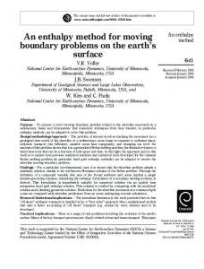
diffusivity in the square capillary tube is considerably higher than the diffusivity for diluted solution, estimated by Scheibel correlation [23], used in previous models [1,2] for diffusivity estimation. Only at the end of the experiment, both diffusivities are similar for the square capillary tube. This behavior can be explained because the driven force is reduced by the dissolved CO2 into the hydrocarbon at this moment. The improved mixing induced by the filaments, may be is also responsible for the higher effective diffusivity in the square capillary tubes. T=296.5K P=200 psig

a)t=0 b)t=60 min Fig.4. Displacement inside square capillary Def [E-9 m2/s]

s(t)-s(0),[mm]

T=296.5K P=200 psig 3.5 3 2.5 2 1.5 1

5

model- cyl

4

model-square

3

diluted solution

2 1 0 0

model-square square exp cyl exp model-cyl

0.5 0 0

20

40

60

80

Fig.7. Effective diffusivity- model results comparison

100

4 Conclusion This more complex mass transfer model, which considers both variable liquid diffusion coefficient and liquid density, is better to represent interface displament in a CO2 diffusion process in liquid nC10, inside capillary tubes. The capillary shape effects can be observed in the variation in the liquid effective diffusivity and in liquid density. The disadvantage against previous simplified models [1,2] is the increase in the simulation time.

Fig.5. Experimental and model results comparison T=296.5K P=200 psig

Liquid Density [Kg/m3]

model-cyl

680 model-square

670

100

tim e [m in]

time [min]

690

50

660

List of Symbols

650

AT= mass transfer area, [m2] Def= Effective CO2 diffusion coefficient in liquid phase, [m2/s]. j= Mass diffusive flux, [kg/(m2 s)] L= capillary tube lenght, [m]. n= Mass total flux, [kg/(m2 s)] P= absolute pressure, [kPa] R= 8.3144 kJ/kmol K s=s(t)= interface position, relative to capillary tube bottom [m]. US= interface velocity,[m/s]. V= Liquid phase volume, [m3] T= temperature, [K] wC= CO2 mass fraction in liquid phase, [-]. yC= CO2 mass fraction in gas phase, [-].

640 0

20

40

60

80

100

time [min]

Fig.6. Liquid density - model results comparison In Fig. 6, a reduction in the liquid density is observed inside both capillary tubes, being more drastic for the square capillary. It can be explained by the presence of the liquid filaments in the corners of the square capillary tube, which improve the mixing in the liquid phase. A similar reduction is observed for the liquid effective diffusivity (Fig.7). However, the effective

ISSN:1790-5109

76

ISBN: 978-960-474-002-4

2nd EUROPEAN COMPUTING CONFERENCE (ECC’08) Malta, September 11-13, 2008

[10] Simmons, M.; Wong, D.; Travers, P.; Rothwell, J. Bubble Behaviour in Three Phase Capillary Microreactors. International Journal of Chemical Reactor Engineering, Vol 1, 2003, A30. [11] Patrick, R. Jr.; Klindera, T.; Crynes, L.L., Cerro, R.L. y Abraham, M.A. Residence time distribution in three-phase monolith reactor. AIChE Journal, Vol. 41, 2004, 649-657. [12] Firincioglu, T.; Blunt, M.; Zhou, D. Three-phase flow and wettability effects in triangular capillaries. Colloids and Surfaces A, Vol. 155, 1999, pp.259-276. [13] Zhou, D.; Blunt, M. y Orr, F. Jr. Hydrocarbon Drainage along Corners of Noncircular Capillaries. J. of Colloid and Interface Science, Vol. 187, 1997, pp.11-21. [14] Illingworth, T.C.; Golosnoy, I.O. Numerical solutions of diffusion-controlled moving boundary problems which conserve solute. Journal of Computational Physics, Vol. 209, N1, 2005, pp. 207-225. [15] Hines, A.; Maddox, R. Transferencia de Masa: Fundamentos y Aplicaciones. Prentice Hall, 1987. [16] Bejan, A. Heat Transfer. John Wiley & Sons, 1995. [17] Unlusu, Betul; Sunol, Aydin K. Modeling of equilibration times at high pressure for multicomponent vapor-liquid diffusional processes. Fluid Phase Equilibria. Vol. 226, 2004, pp. 15-25. [18] Sassi, M.; Raynaud, M. Solution of the movingboundaries problems. Numerical Heat Transfer Part B, Vol.34, 1998, pp.271-286. [19] Wilke, C.; Lee. Ind.Eng.Chem. Vol.47, 1955, pp.1253. [20] Pitzer, K.S.; Sterner, S.M. Equations of state valid continuously from zero to extreme pressures for H2O and CO2. J.Chem.Phys. Vol. 101 (4), 1994, pp. 3111-3116. [21] Reamer, H.; Sage, B. Phase equilibria in hydrocarbon systems. Volumetric and phase system. behavior of the n-decane-CO2 J.Chem.Eng.Data. Vol. 8, 1963, pp. 508-513. [22] Zabala, D.; López de Ramos, A. Solute concentration effect in gas-liquid interface displacement modeling. WSEAS Transactions on Fluid Mechanics. Vol. 1, Nº 6, 2006, pp. 686691. [23] Scheibel, E.G. Ind.Eng.Chem. Vol.46, 1954, pp. 2007.

Greek letters ρk= mass density of “k” phase, [kg/m3]. Subscripts L= liquid phase G= gas phase

Superscripts ini= initial sat= saturation

Acknowledgement The authors want to thank CDCH-Universidad de Carabobo (Project Nº 2007-001) and Fonacit (S12001-000778) for their financial support. References: [1] Zabala, D.; López de Ramos, A. Effect of the Finite Difference Solution Scheme in a Free Boundary Convective Mass Transfer Model. WSEAS Transactions on Mathematics, Vol.6, Nº 6, 2007, pp.693-700. [2] Zabala, D.; López de Ramos, A. Solute concentaration effect in gas-liquid interface displacement modeling. WSEAS Transactions on Fluid Mechanics, Vol.1, Nº 6, 2006, pp. 686-691. [3] López de Ramos, A. Capillary enhanced diffusion of CO2 in porous media. Ph.D. Dissertation, University of Tulsa, U.S.A, 1993. [4] Grogan, A.; Pinczewski, V.; Ruskauff, G.; Orr, F. Diffusion of carbon dioxide at reservoir conditions: Models and Measurements. Paper SPE/DOE 14897, presented at SPE/DOE Fifth Symposium on Enhanced Oil Recovery, Tulsa, OK, Apr. 20-23, 1986. [5] Garrido, A. Estudio Teórico Experimental de la Transferencia de Masa en Líquidos Confinados en Regiones con Angularidades. M.Sc Thesis, Universidad Simón Bolívar, Venezuela, 2005. [6] De Freitas, A. Estudio del efecto de las esquinas en la transferencia de masa en medios porosos. M.Sc Thesis, Universidad Simón Bolívar, Venezuela, 2005. [7] Lenormand, R.; Zarcone, C. Role of roughness and edges during imbibition in square capillaries. Paper SPE 13264, presented at the 59th Annual Technical Conference and Exhibition of the Society of Petroleum Engineers of AIME, Houston, Texas, Sept. 16-19, 1984. [8] Patzek, T.W.; Kristensen, J.G. Shape Factor and Hydraulic Conductance in Noncircular Capillaries I: One-Phase Creeping Flow. J. of Colloid and Interface Science, Vol. 236, 2001, pp.295-304. [9] Patzek, T.W.; Kristensen, J.G. Shape Factor Correlations of Hydraulic Conductance in Noncircular Capillaries II: Two-Phase Creeping Flow. J. of Colloid and Interface Science, Vol. 236, 2001, pp.305-317.

ISSN:1790-5109

77

ISBN: 978-960-474-002-4