Variable Digital Filters Georgi Stoyanov and Masayuki Kawamata Graduate School of Engineering, Tohoku University, Aoba, Aramaki, Aoba-ku, Sendai 980-77, Japan E-mail:
[email protected] Abstract There has been a constant interest in the design and implementation of digital filters with variable characteristics for different applications. In this article an attempt is made to review and systematize all known structures and methods of design of such filters. First the basic theory of the variable digital filters is introduced. Then FIR and IIR realizations with real and complex coefficients are considered, the known results for multidimensional variable filters are discussed and finally, typical implementations are overviewed. Recommendations for applications in different situations are given and unresolved problems are pointed out. This work is basically a review, but some of our original results are also included. Keywords: Variable/tunable digital filters, FIR and IIR filters, complex coefficients, 1-D and 2-D digital filters
1. Introduction H(ω)
In many signal processing applications a clear need to change the parameters of the filters used exists. Such applications are found in telecommunications, digital audio equipment, medical electronics, radar, sonar and control systems, adaptive and tracking systems, spectrum and vibration analyses, formant speech synthesizers and in numerous laboratory instruments. The most general term for filters with changeable parameters is “variable filters”, but they are often called “tunable” (although this term is correct only when frequency-related parameters are the subject of change), “adjustable” (this term is correct only for changes in some narrow range of values of a given parameter) or “programmable” (when parameters can be reprogrammed or are controlled by a computer). In analog variable filters, tuning is often achieved by trimming some passive element and thus the term “trimmed” is also used to refer to the filter. There are many limitations and technical problems in realizing passive variable filters. The realization is easier with active filters (especially for filters with programmable parameters), but it becomes an easy task with practically unlimited possibilities in the case of digital variable filters. In the most general case of a variable filter, all filter magnitude parameters (Fig. 1) might be subject to changes. Variable magnitude deviations δs (in the stopband) and δp (in the passband) are, however, not easily achievable – complicated recalculations of the entire transfer function are required and usually many circuit elements must be changed in order to obtain the new δs and δp. Fortunately, more often, only frequency parameters – cutoff frequency ωc and stopband edge ωs of lowpass (LP) and highpass (HP) filters (Fig.1a) or ωc1, ωc2, ωs1,
1 1-δp
H(ω) 1 1-δp
δp
δp BW
δs1
ωc
ωs
δs
ω
ωs1
ωc1 ω0 ωc2 ωs2
δs2
ω
Fig. 1. Illustration of the possible variable magnitude response parameters for (a) low-pass filter; (b) band-pass filter.
ωs2, center frequency ω0 and bandwidth BW (Fig. 1b) of bandpass (BP) and bandstop (BS) filters – are tuned. This is an easier task compared with all-magnitudeparameters tuning and it can be further simplified, for example, by keeping BW constant and tuning only ω0, or by tuning BW and ω0 independently. The rare case in which the entire magnitude response is varied, is the magnitude equalizer. The magnitude response in this case, however, is easily decomposed into a product of first- and second-order components described by simple frequency parameters such as ω0 and BW, which are usually tuned without problems. Thus any arbitrary magnitude response could be obtained by varying the frequency parameters ω0i and BWi . It should be noted that the magnitude responses of magnitude equalizers change gradually (no sharp jumps) compared to most other filters and thus they have lower values of the transfer function quality factors. This facilitates the implementation and reduces the problems of tuning and of stability control during the tuning process. Finally, there is another group of variable circuits with constant magnitude, where only the phase response (group delay time) is varied. These are called
phase equalizers, but they will not be discussed in this paper. The first publications concerning variable digital filters date back to the early 70’s [1]-[5] and the problems were already more generally treated in the early 80’s [6]-[9]. Nowadays there are already hundreds of publications and there is a need to systematize the collected knowledge – the methods proposed and structures developed. This is the first aim of the present work. Then, we try to compare all the methods and structures available, and finally, some recommendations concerning the usage of the known results are given and unresolved problems are pointed out. Since this work is addressed to a wide audience, we try to maintain a tutorial manner of presentation, but some of our original results are also included.
2. Basic Theory Most of the design methods for digital filters with variable cutoff and center frequencies are based on different transformations applied to a prototype (usually LP) filter. The most popular are the spectral transformations, proposed by Constantinides [2], and the transformations proposed by Oppenheim et al. [3]. The spectral transformations of Constantinides [2] are based on the substitution z −1 → T ( z ) . (1) Thus, starting from a LP prototype filter with a cutoff frequency ωcp and transfer function Hp(z), M
H p ( z) =
∑ ai z i
i= 0 N
1+
∑ bj z
−j
(IIR) or H p ( z ) =
N −1
∑ ai z i ,
(FIR)
i =0
j =0
and applying (1), it is possible to obtain a LP, HP, BP or BS filter with a new transfer function H ( z ) = H p ( z ) z −1 =T ( z ) (2) and variable cutoff frequencies. For LP to LP and LP to HP transformations, T(z) is T (z) = β LP = β HP =
z −1 m β
sin[( ω c p + ω c ) / 2 ]
(3)
;
k = cot
ωcp (ω c2 − ω c1 ) , tan 2 2
and
T(z) =
z−2 −[2β / (k +1)]z −1 + (1− k) / (1+ k) (1− k) / (1+ k)z −2 −[2β / (k +1)]z−1 +1
, (5)
where
βBS = cosω0 = βBP ; k = tan[(ωc2 − ωc1) / 2]tan(ωcp / 2). In fact, T(z) are first- (3) and second-order (4), (5) allpass transfer functions, and this accounts for the other name of these transformations, “allpass transformations”. It is then easy to generalize T(z) to an allpass transfer function of any order N [10], N
∑ ai z i − N
T ( z ) = ± i =N0
∑ ai z − i
,
(6)
i= 0
and to use it in the design of multiband filters. The transformation of Oppenheim et al. [3] starts from a zero-phase FIR filter with transfer function H0(z) and symmetric impulse response h0(n) = h0(-n). Any linear-phase FIR filter with transfer function H(z) and impulse response h(n) of length 2N+1 can be expressed through H0(z) and h0(n) [3]: H ( z ) = z − N H 0 ( z ); h( n ) = h0 ( n − N ); N (7) z + z −1 n ) , H 0 ( z ) = ∑ a( n )( 2 n=0 where the coefficients a(n) are related to h0(n) through the coefficients of Chebishev’s polynomials Cn(x) of the n-th order. The frequency responses corresponding to (7) are H(ejω)= ejωΝΗ0(ejω); Η0(ejω)=
N
∑ a( n )(cos ω )n . (8)
n=0
cos[( ω c p + ω c ) / 2 ]
z −2 − [2βk / ( k + 1)]z −1 + ( k − 1) / ( k + 1) ( k − 1) / ( k + 1)z − 2 − [2βk / ( k + 1)]z −1 + 1
cos ω =
P
∑ Ak (cos Ω )k ,
(9)
k =0
where Ω is the frequency scale of the transformed filter.
− cos[( ω c p − ω c ) / 2 ]
with a “minus” sign in T(z) for LP to LP and a “plus” sign for LP to HP transformations. ωc in (3) is the desired cutoff frequency of the new LP or HP filter. For LP to BP and LP to BS transformations, respectively, T(z) = −
cos [( ω c1 + ω c2 ) / 2] , cos [( ω c2 − ωc1 ) / 2]
β BP = cos ω0 =
The transformation of Oppenheim et al. [3] is based on the substitution of variables
;
1 m β z −1 sin[( ω c p − ω c ) / 2 ]
where
;
(4)
If Z = e jΩ is the z-variable corresponding to Ω, the new transfer functions H0(Z) and H(Z) will also have linear phases and symmetric impulse responses like those of the starting transfer functions (7). The first relation in (7), however, changes to H(Z) = Z-NPH0(Z) and the length of the new filter becomes 2NP+1. The frequency response of this filter, on the other hand, may
vary with variations of coefficients Ak (9) and it could be used for tuning the new filter. For the first-order transformation (9) (P = 1), cos ω = A0 + A1cos Ω ,
(10)
the length of the new filter will be the same (2N+1) and the two coefficients A0 and A1 will control the frequency response. An additional restriction, A0+A1=1, which makes the DC gain invariant, reduces the transformation to a single parameter one: cos ω = A0 + (1 − A0 )cos Ω . (11) If the prototype filter is LP with cutoff frequency ωc, the transformed filter will have a cutoff frequency [3], cos ω c − A0 , (12) Ωc = cos−1 1 − A0 which is easily controlled by changing A0. In z-variable transformation (9) becomes P z + z −1 Z + Z −1 k = ∑ Ak ( ) (13) 2 2 k +1
.
3. Variable FIR Digital Filters 3.1. Filters based on Oppenheim et al.’s transformation Transformation (9), (13) is developed for the design of variable cutoff frequency linear-phase FIR digital filters and it is applied to Taylor’s structure [3] (Fig. 2a). For first-order transformation, (13) changes to z + z −1 Z + Z −1 = A0 + A1 , (14) 2 2 and it produces the structure shown in Fig. 2b. Its cutoff frequency can easily be changed by changing A0 and A1. Another approach is to decompose Taylor’s structure into a cascade connection of fourth-order sections and to apply transformation (14) to each of them. It is shown in [4] that Oppenheim et al.’s transformation is good only for the range of values of dΩ/dω (calculated from (10)) within the limits 1 ≤ dΩ/dω ≤ 2. x(n)
1 + z −2 2
a(0)
a(1) z-1
(a)
x(n)
z
a(0) (b)
Ao +
-2
z-1
a(N)
a(N-1) z-1
+
z-1
1 + z −2 2
1 + z −2 2
z-1
+
+
A1/2
-2
z
a(1)
a(N-1) +
z-1
y(n)
Ao
z-1
+
+
+
A1/2 a(N) +
y(n) Fig. 2. Variable cutoff frequency linear-phase FIR filter: (a) Taylor structure; (b) variable structure obtained after applying first-order transformation (9), (13).
For a higher-order transformation (13), the “0.5(1+Z2)”-branches in Fig. 2a will be replaced by circuits of order P and the “z-1”-branches - by “Z-P”branches [3]. Thus the order of the final filter increases P times. The case of a single parameter (11) was investigated in [7] and it was found that the cutoff slope of the variable filter decreases when the cutoff frequency increases during tuning. Thus the frequency range over which the filter is tuned, may be considerably narrowed. This drawback, together with another one – having Ωc≥ωc – could be avoided if second-order transformation (9), (13) is used: (15) cos ω = A0 + A1cosΩ + A2 cos2Ω . The conditions A1 = 1 and A0 = A2 are often introduced in order to preserve the number of variable parameters and the volume of computations. In all cases up to now, only LP prototypes and LP variable filters have been considered. In [11] this approach is extended to linear-phase BP prototypes and linear-phase BP variable filters. If ωc1 and ωc2 are the cutoff frequencies of the prototype filter (Fig. 1b) and Ωc1 and Ωc2 are these of the transformed filter, it is easy to derive, from (10), A0 = cos ω c1 − A1cos Ω c1 ,
(16)
A1 = ( cos ω c1 − cos ω c2 ) / ( cos Ω c1 − cos Ω c 2 ) . (17) Thus, it becomes possible to tune the center frequency or the bandwidth by varying only the parameter A1. It is generally not possible to change the center frequency while keeping the bandwidth constant, but some ways of achieving this are suggested in [11]. Another approach to obtaining tunable BP filters from LP (not from BP as in [11]) prototypes, was given in [12], based on which transformation (10) is modified to sin (ω/2) = A0 + A1cos Ω (18) and the cutoff frequency ±ωc of the LP prototype is mapped to ±Ωc1 and ±Ωc2. Then Ωc1 and Ωc2 are controlled by changing A0 and A1. Variable LP and HP filters, considered as special cases of BP filter, can also be designed using this approach. The prototype circuit, used in [12] has the same Taylor structure as in Fig.2a. Relations (16) and (17) are used in [13] (where (14) is called the Mobius transformation) as a starting point in the development of variable cutoff frequency linearphase filters that are not based on the Taylor structure. The final result, however, is not a FIR filter. 3.2. Direct-form FIR variable filters All known variable filters, based on Oppenheim et al.’s transformation, are realized as transformed Taylor’s structures (Fig. 2). The final circuit is quite specific, often not desirable, and, for higher-order transformation (13), too complicated. Neither is there a
simple relation between the filter coefficients and the cutoff frequency, which makes the hardware implementations difficult and impractical. Another approach for producing direct-form linearphase FIR variable filters with a simple relationship between filter coefficients and the cutoff frequency, was advanced by Jarske et al. [14], [15]. Starting from the impulse response nid(n) of an ideal LP filter, Jarske et al. applied the following approximation for the impulse response h0(n) of a LP filter with equal ripples δp and δs (Fig. 1), used as a prototype: for n = 0 c( n )ω c + d h0 ( n ) = c( n )sin ( nω c ) for 1 ≤| n|≤ N 0 otherwise ,
(19)
where ωc is the variable 6 dB cutoff frequency, c(-n)=c(n) for |n|(0 and d is a constant. Coefficients c(n) are determined in the design procedure and d is used to adjust HP and BS filter responses (d=0 for an ideal LP filter). It appears from (19) that the center coefficient h0(0) is a linear function of the cutoff frequency, and that all h0(n) coefficients are also simple functions of ωc. h0(n) might be obtained using either a window-based (h0(n)=w(n)hid(n), where w(n) could be any symmetric window) or optimal (using the Remez exchange algorithm) method of design. When optimal designs are used, however, for filters of even-length 2N, a better approximation is [15] h0(n) = c(n)sin [ωc(n-0.5)],
(20)
where -N+1≤n≤N and c(-n+1)=-c(n), and it is recommended to have equal weights in both the passband and the stopband. Another detail in the case of optimal design is that first an optimal LP filter h00(n) with 6 dB cutoff frequency ωc0 is designed with ωc0 chosen in such a way as to ensure that all coefficients h00(n) are nonzero. Jarske et al. [15] proposed ωc0 = 2π[0.25+0.5(2N+1)] for odd-length 2N+1 ωc0 = 0.5π for even-length 2N. (21) Then, coefficients c(n) for (19) and (20) are calculated as h00 ( n ) for n ≠ 0 and odd length sin ( nω ) c0 c( n ) = (22) h00 ( n ) for even length, sin[( n − 0.5)ω c 0 ] where c(0)=1/π for odd length. For a LP prototype with odd-length 2N+1, a zerophase HP filter can be obtained as its amplitude complementary. This filter will have the same cutoff frequency ωc0 as that of the LP filter (which is easily made variable), and impulse response [15]
1 − h0 ( n ) for n = 0 hHP0 ( n ) = − h0 ( n ) for 1 ≤| n| ≤ N .
(23)
The BP filter can be obtained by using a modulation scheme, and it will have impulse response hBP0 (n) = 2cos (ω0n) h0 (n),
(24)
where ω0 is the desired center frequency (Fig.1b) introduced by the modulation scheme. The BS filter is easily designed by combining (23) and (24), while a notch filter can be obtained by taking the difference between the prototype LP filter and its complementary filter. The impulse response of such a notch filter is [15] 2h0 ( n ) − 1 for n = 0 hN 0 ( n ) = (25) 2h0 ( n ) for 1 ≤| n| ≤ N . For even-length 2N, expressions (23) and (24) change to hHP0(n) = cos (nπ) h0(n)
0