false positive rate (FPr). However, due to the neces- sary interpolation, the corresponding âvirtualâ operat- ing points cannot yield deterministic decisions. This.
Variance estimation for two-class and multi-class ROC analysis using operating point averaging Pavel Pacl´ık, Carmen Lai, Jana Novoviˇcov´a, Robert P.W.Duin PR Sys Design, Delft, The Netherlands Institute of Information Theory and Automation, Czech Academy of Sciences, Prague, Czech Republic Information and Communication Theory Group, TU Delft, The Netherlands
Abstract Receiver Operating Characteristic (ROC) analysis enables fine-tuning of a trained classifier to a desired performance trade-off situation. ROC estimated from a finite test set is, however, insufficient for the sake of classifier comparison as it neglects performance variances. This research presents a practical algorithm for variance estimation at individual operating points of ROC curves or surfaces. It generalizes the threshold averaging of Fawcett et.al. to arbitrary operating point definition including the weighting-based formulation used in multi-class ROC analysis. The statistical test comparing performance differences between operating points of the same curve is illustrated for two-class and multiclass ROC.
1. Introduction Receiver Operating Characteristic (ROC) analysis facilitates fine-tuning of a trained classifier to the application-specific optimum based on estimation of performance trade-offs. ROC estimated from a finite test set is, however, insufficient for the sake of classifier comparison as it lacks information on performance variability. Area under ROC curve (AUC), averaged over multiple cross-validation folds is currently the most common technique for ROC-based model comparison. The shortcoming of this approach is that AUC integrates evidence over all or a subset of operating points. Therefore, it is of no value for performance variation assessment at a specific operating point, which is a typical goal of industrial practitioners. In this paper, we describe the procedure for estimation of ROC with variances applicable to both two-class and multi-class situations. Number of researchers addressed the problem of variance estimation in ROC analysis. Provost 1998 et al. [6, 2] proposed the vertical averaging where the
true positive rate (T P r) is viewed as a function of the false positive rate (F P r). However, due to the necessary interpolation, the corresponding “virtual” operating points cannot yield deterministic decisions. This problem is alleviated by the threshold averaging approach of Fawcett et al. [2]. Fawcett proposes to generate multiple ROC-estimation sets using cross-validation (with replacement) or bootstrapping and to estimate the distribution of ROCs. By merge-sorting all thresholds of all ROCs, a single threshold pool is derived. For each threshold of the sub-sampled pool, Fawcett looks up the corresponding thresholds in the original ROCs and averages the respective error estimates. As the threshold averaging leverages genuine (not virtual) operating points, it allows one to directly perform decisions at arbitrary point of the ROC. Disadvantage of this approach, which motivated our research, is that the algorithm relies on ordering of the soft outputs of the classifier and is thereby applicable only to the two-class problems using threshold-based decisions. The contribution of this paper is two-fold. Firstly, we extend the threshold averaging to arbitrary operating point definition including the weighting-based formulation used in multi-class ROC analysis. Secondly, we propose the procedure incorporating both the ROC construction and ROC variance estimation in a single cross-validation session. Instead of sampling with replacement or bootstrapping, we adopt the n-fold rotation scheme. This allows us to produce a single set of unbiased soft output estimates using Wolpert’s stacked generalization technique [9]. The ROC analysis, performed at this stacked generalized set, results in a set of classifier operating points. Consequently, the per-fold trained classifiers yield decisions for the respective fold test sets at the identical set of operating points. This removes the need for operating point ordering or threshold matching. Averaging the error estimates of each fold, we compute the mean ROC with variances. In order to illustrate applicability of the operating
point averaging, we propose the statistical test comparing the operating points on the same ROC. The test enables us to define a subset of the ROC where the performance differences are insignificant with respect to the operating point of interest. We demonstrate, that this method may help us to assess whether the available sample size is sufficient to differentiate between operating points.
2. Classifier operating points and ROC Consider a classification problem with C classes, ω1 , ω2 , · · · , ωC , with input data x ∈ RD . For the sake of this discussion, we focus on classifiers producing soft outputs such as an estimate of class membership probability or distances to the decision boundary. The output of the trained classifier Ψ is usually a vector y = {y1 , . . . , yC } of continuous values. In case of twoclass problem, the output of the classifier Ψ may be a scalar y ∈ R. Decision rule ∆ is a mapping of the soft output y to the decision Ω: ∆(y | φ) : y → Ω, where Ω = {ω1 , · · · , ωC }. The set of decision rule parameters φ is called operating point. In case of the scalar soft output, the operating point may be defined as φthr = {θ, ω t , ω nt }, where θ denotes the threshold, and symbols ω t and ω nt refer to the target and non-target class, specified by the trained classifier Ψ. Assuming that the classifier output is similarity, the decision function may be defined as: ( ωt if y ≥ θ (1) ∆thr (y | φthr ) = nt ω otherwise. Operating point for a vector soft output is a set of per-class weights φw = {w1 , . . . , wC }, wc ≥ 0, c = 1, . . . , C. The class assignment is now based on each output yc multiplied by the corresponding weight wc : C
∆w (y | φw ) = arg max wc yc . c=1
(2)
The classical ROC curve depicts the trade-off between the true positive rate (T P r) and the false positive rate (F P r) [2]. Other performance measures yield ROC alternatives, such as the precision-recall operating characteristics adopted for information retrieval [7]. Compared with the ROC analysis, the alternative measures may introduce new qualities such as sensitivity to class prior probabilities [4]. For the sake of this discussion, we adopt a broader definition of ROC as a set of relevant operating points, selected from a test set, accompanied with a set of performance measures estimated at these points.
3. Operating point averaging Algorithm 1 outlines the proposed ROC estimation scheme Algorithm 1 Operating point averaging 1: Input: Labeled dataset, classification algorithm, number of folds n. 2: Perform n-fold stratified cross-validation. In each fold use all but one part to train a classifier. Execute the trained classifier on the fold test set and store the soft outputs. 3: Collect the per-fold soft outputs into a single set (stacked generalization). 4: Construct ROC on the stacked generalized outputs. 5: For each operating point φi of the estimated ROC 6: For each fold f = 1, ..., n 7: Perform decisions on the per-fold soft outputs. 8: Estimate confusion matrix using the groundtruth labels and the decisions. 9: Compute desired performance metrics. 10: Next fold 11: For each performance measure, estimate its mean and variance at φi . 12: Next operating point 13: Output: Set of operating points Φ, set of performance measures with means with variances. The key aspect of the algorithm is adoption of the nfold stratified cross-validation scheme. It allows us to stack-generalize the soft outputs of classifiers trained in all folds into a single set [9] and perform the single ROC analysis on these outputs. Operating points, defined by the step (4) are then leveraged to estimate the per-fold performances of interest. The resulting means and standard deviations of the performances form, together with the used set of operating points, the resulting ROC.
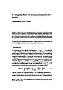
4. Experiments 4.1. Illustration of operating point averaging This experiment illustrates the proposed algorithm for ROC variance estimation on the artificial Highleyman data set [3, 1]. This data set is composed of two Gaussian classes with means µ1 = [1, 1] and µ2 = [2, 0] and covariance matrices Σ1 = [1, 0; 0, 0.25] and Σ2 = [0.01, 0; 0, 4]. We are interested in estimating ROC for the Gaussian detector on class 1 using the decision function in Eq. 1 (ω t = class 1, ω nt = class 2). We perform 10-fold stratified cross-validation and for each fold test set collect the probability densities of the Gaussian model. We sub-sample the unique values
of the 200 soft outputs, available in the stacked generalized set, and construct the ROC with 30 operating points. For every point, we perform decisions in each per-fold set of soft outputs. The estimated ROC composed of the mean F P r and T P r measures and the standard deviations of the means is presented in Figure 1. 1 0.9 True positive ratio (TPr)
0.8 0.7 0.6 0.5 0.4 0.3 0.2
Two sub figures in Figure 2 present ROC curves with variances estimated on the Highleyman dataset with 50 and 200 examples per class, respectively. The ROC with 30 operating points is generated by thresholding the Gaussian model output on class 1. On each curve, we manually select the operating point φs with T P r of at least 0.9 (cross marker). The above mentioned t-test is then performed for each ROC comparing the selected point to every other point on the same curve. The circle markers denote the operating points for which the null hypothesis was accepted at the confidence level of 95%. We conclude that the F P r at these operating points is not significantly different from the selected one. The effect of larger sample size may be observed in the sub figure b). For the larger data set with 200 examples per class, the selected operating point is significantly different from the neighboring points.
0.1 0
0
0.2
0.4 0.6 False positive ratio (FPr)
0.8
1
Figure 1. Mean ROC with standard deviations of the mean estimated for the Gaussian detector on class 1 of the Highleyman problem
4.2. Significance test In order to compare the performance of the same classifier at two operating points, we need a statistical test to decide whether performance differences are significant. Because the performances at two operating points of the same classifier exhibit statistical dependence, we adopt the t- test for two dependent samples. Let Xφi and µXφi denote the performance measure and true mean performance measure of the classifier at the operating point φi , i=1,2, respectively. The test statistics for the test with null hypothesis H0 : µXφ1 = µXφ2 against non-directional alternative is [8]: t= q
¯φ − X ¯φ X 1 2 s2X¯
φ1
+ s2X¯
φ2
− 2rXφ1 Xφ2 (sX¯ φ1 )(sX¯ φ2 )
. (3)
¯ φ and sX¯ denote the estimated mean and stanHere X i φi dard deviation computed for the operating point φi , i = 1, 2, and rXφ1 Xφ2 represents the estimated coefficient of correlation between Xφ1 and Xφ2 . If rXφ1 Xφ2 = 0 then the test statistic (3) becomes identical to the test statistic for the t-test using independent samples. The degree of freedom for the t-test is 2n − 2, where n is the number of cross-validation folds in Algorithm 1. We apply the test separately for each performance measure and thus do not account for possible covariances between the measures.
4.3. Significance test for three-class ROC This example illustrates applicability of the proposed approach in a multi-class situation. In order to facilitate ROC visualization, we use a three-class problem comprising handwritten digit ’2’, ’3’, and ’5’ 1 . The digits are represented by six morphological features. The design dataset contains 100 examples per class. The studied algorithm is composed of the PCA feature extraction projecting the input data into 3D subspace, followed by the Bayes quadratic classifier (QDC). The weighting-based decision function is applied, defined in Equation 2. We estimate the three-class ROC with variances using the proposed operation point averaging based on 10-fold cross-validation. The ROC is constructed using the greedy search minimizing the maximum per-class error2 . Starting from 1000 randomly generated weight vectors, five greedy steps are run each retaining the top 100 operating points with the smallest maximum per-class error. Figure 3 depicts the 3D ROC visualizing the per-class errors for the subset of the top 100 returned operating points with lowest perclass errors. The plot omits the estimated error bars for the sake of clarity. Similarly to the previous example, the cross-marker denotes the manually-selected operating point of interest. In this experiment, we perform the t-test for each of the three per-class errors. The circle markers highlight the operating points for which the above-mentioned null hypothesis got accepted at the 95% confidence level for all the three per-class errors (AND operator). We conclude that the available sample size is insufficient in 1 http://archive.ics.uci.edu/ml/datasets/Multiple+Features 2 For more robust multi-class ROC estimation algorithm, applicable to large number of classes see [5]
1 0.9
0.8
0.8 True positive ratio (TPr)
True positive ratio (TPr)
1 0.9
0.7 0.6 0.5 0.4 0.3 0.2
0.6 0.5 0.4 0.3 0.2
manually!selected operating point op.point with equal FPr at 95% level
0.1 0
0.7
0
0.2
0.4 0.6 False positive ratio (FPr)
0.8
(a) Design set with 50 samples per class
1
manually!selected operating point op.point with equal FPr at 95% level
0.1 0
0
0.2
0.4 0.6 False positive ratio (FPr)
0.8
1
(b) Design set with 200 samples per class
Figure 2. Testing statistical significance of differences between F P r of the manually-selected operating point at T P r=0.9 and the remaining points on the ROC with variances.
order to distinguish differences between the operating points in the the demarcated neighborhood.
Acknowledgments Authors would like to thank Rina Nir from Advanced Medical Diagnostics for support.
References 0.7
error on digit ’5’
0.6 0.5 0.4 0.3 0.6 0.4 0.2 error on digit ’3’
0
0
0.05
0.1
0.15
0.2
0.25
0.3
error on digit ’2’
Figure 3. Testing significance of performance differences for three-class ROC
5. Conclusions In this paper, we provide a general algorithm for estimation of ROC with variances at each operating point. The algorithm bears similarity to the threshold averaging of Fawcett et al. adding two important improvements. Firstly, it is applicable to arbitrary definition of the operating point and both two-class and multi-class ROC analysis. Secondly, we illustrate the practical applicability of the proposed scheme for testing of performance differences between operating point of the same ROC. The proposed test, taking into account dependencies between operating points of the same classifier, enables one to assess whether the available sample size is sufficient for differentiating between a group of operating points.
[1] R. P. W. Duin, P. Juszczak, D. de Ridder, P. Pacl´ık, E. Pekalska, and D. M. J. Tax. PR-Tools 4.1, a Matlab toolbox for pattern recognition. Technical report, ICT Group, TU Delft, The Netherlands, August 2007. http://www.prtools.org. [2] T. Fawcett. An introduction to ROC analysis. Pattern Recognition Letters, 27(8):861–874, 2006. [3] W. Higleyman. Linear decision functions, with application to pattern recognition. In IRE, pages 49:31–48, 1961. [4] T. Landgrebe, P. Pacl´ık, A. Bradley, and R. Duin. Precision-recall operating characteristics P-ROC curves in imprecise environments. In Y. Tang, S. Wang, G. Lorette, D. Yeung, and H. Yan, editors, 18th Int.conf. on Pat.Rec., volume 4, pages 123–126. IEEE Computer Society Press, Los Alamitos, 2006. [5] T. C. W. Landgrebe and R. P. W. Duin. Efficient multiclass ROC approximation by decomposition via confusion matrix perturbation analysis. IEEE Trans.on Pattern Analysis and Machine Intelligence, 30(5), May 2008. [6] F. Provost, T. Fawcett, and R. Kohavi. The case against accuracy estimation for comparing induction algorithms. In J. Shavlik, editor, ICML-98, volume Morgan Kaufmann, San Francisco, CA, pages 445–453, 1998. [7] V. Raghavan, P. Bollmann, and G. S. Jung. A critical investigation of recall and precision as measures of retrieval system performance. ACM Trans. Inf. Syst., (7):205–229, 1989. [8] D. J. Sheskin. Handbook of Parametric and Nonparametric Statistical Procedures. Chapman & Hall/CRC, 3rd edition edition, 2003. [9] D. Wolpert. Stacked generalization. Neural Networks, 5:241–259, 1992.