of an online estimation algorithm we recently investigated theoretically. One of the peculiar .... Roumeliotis and Bekey [8] proposed to split the overall EKF1 into n.
Online estimation of variance parameters: experimental results with applications to localization Gorkem Erinc, Gianluigi Pillonetto, Stefano Carpin
Abstract— This paper presents an experimental validation of an online estimation algorithm we recently investigated theoretically. One of the peculiar characteristics of the approach we propose is the ability to perform an online estimation of the variance parameters that regulate the dynamics of the nonlinear dynamical model used. The approach exploits and extends classical iterated Kalman filtering equations by propagating an approximation of the marginal posterior of the unknown variances over time. The method has been previously used to model and solve a localization task for multiple robots equipped only with a sensor returning mutual distances. In this paper we present a first experimental validation of the algorithm that complements and confirms our initial promising theoretical findings. Our current implementation relies on a sensor returning distance estimates based on a simple image processing algorithm. Such sensor is inherently and intentionally noisy, and in this study we show that our technique is capable of appropriately estimating the variance describing the noise affecting this sensor. We conclude proving experimentally that the procedure we present ensures a performance comparable to similar algorithms that require significantly more a priori information.
I. I NTRODUCTION Tomorrow’s society will see the deployment of more and more networked robots interacting among themselves and with low cost devices dispersed in the environment. The area of multi-robot systems steadily grew in the last fifteen years, and multi-robot solutions appear to be the winning choice for many different tasks [1]. More recently, a vigorous evolution in sensor networks have opened the doors to more intriguing scenarios where robots no longer just interact with other robots, but exchange information also with sensors scattered in the environment. These sensors may have been a priori deployed, or even positioned by the robot themselves while operating. The interaction between research in multi-robot systems and sensor networks appears to be one of the most exciting ones for the near future. These considerations are the basis for the research generating the results presented in this manuscript. In particular, we aim to develop multirobot systems capable of completing complex tasks while operating in unstructured environments not offering features appropriate to solve the localization task. In this case, it is appealing to envision that robots will instead deploy a suitable supporting sensor network while operating, or that robots themselves will constitute the localization infrastructure. The reader should note that in this line of research we do not assume the availability of sensorial payload Gorkem Erinc and Stefano Carpin are with the School of Engineering, University of California, Merced, USA. Gianluigi Pillonetto is with the Department of Information Engineering, University of Padova, Italy.
suitable to solve the full pose estimation based on SLAM algorithms producing two dimensional or three dimensional maps. Eventually, our goal is to use distance sensors based on time of flight like those being anticipated in [2]. When these sensors will be available, they will be deployed in the environment at run time, and treated as consumable components. Therefore, it would be not viable to invest significant time before hand to derive an accurate statistical model describing their performance. It is rather much more appealing to infer this statistical description online, while the robot uses these sensors. Starting from this scenario, we have recently developed an estimation algorithm compatible with these assumptions [3]. Its main strength is in the ability to estimate online the parameters characterizing the variance of the transition and measurement noise. We have already shown that such method can be used to solve a multi-robot localization problem where robots are only equipped with sensors returning mutual distances. We assumed that at every point in time some of the robots move whilst the others stand still in order to serve as fixed landmarks for the moving ones. A thorough theoretical investigation has shown that the method is capable of reliably estimating the covariance matrices of transition or measurement noise (but not both at the same time). Results based on extensive simulations also suggested that the algorithm behaves favorably when compared to the extended Kalman filter (EKF) and the iterative Kalman filter (IKF), even though it requires much less a priori information. In this paper we provide the first experimental validation of the proposed technique. Accordingly to our future plan involving deployable landmarks, we here exclusively focus on estimating the covariance of the measurement noise. In particular, we have implemented a vision based sensor that returns distance to visual landmarks based on a simple image processing algorithm. Our aim is to prove that the technique we have theoretically investigated is viable also from a practical point of view when implemented on real world systems. As detailed in the subsequent sections, it turns out that this is the case. The remaining of the paper is organized as follows. Related literature is presented in section II. The estimation problem and algorithm is shortly summarized in section III. Our original general purpose formulation is therein reworked in order to take into account the specific scenario considered. The experimental setup is described in section IV. Finally, conclusions and future work are proposed in section V.
II. R ELATED WORK
III. N OTATION , PROBLEM DEFINITION , AND THE
Localization is one of the most widely studied topics in mobile robotics. Since in our experimental setup we focus on mobile robots moving in planar environments, we restrict our discussion to techniques aimed to determine the position in the plane and the yaw orientation of the robot. In other words we look at algorithms that estimate the triple (x, y, θ), indicated as pose in the following. The recent book by Thrun et al. [4] offering an up to date description of the most commonly used probabilistic techniques adopted to solve this problem reveals that most of the published literature in the field resorts to some implementation of the Bayes filter. In multi-robot localization, relevant for our experimental setup, the aim is to localize n robots moving in a shared environment and equipped with some sensors to detect not only the environment but also their mutual positions. While this problem can be solved by running n independent instances of the formerly described methods, or a single filter estimating the 3n components of the composed state, research has been done towards the development of cooperative localization. The term was introduced by Rekleitis et al. that first considered two robots using visual sensors to reduce odometry errors [5], and later on considered more than two robots and different sensors [6]. Howard et al. also considered the cooperative localization problem, using a maximum likelihood estimator instead [7]. Roumeliotis and Bekey [8] proposed to split the overall EKF1 into n smaller communicating filters allocated on the n robots in the team. More recently, Mourikis and Roumeliotis [9], [10] investigated the intrinsic limitations of these approaches. In particular they relate the localization accuracy to available resources, like the amount of exchanged information, sensing frequency, and so on. When the environment offers no features, two strategies can be used in order to install a suitable infrastructure. When more robots are available, some of them could serve as artificial detectable features. This idea was pioneered by Kurazume, Hirose et al. [11], and by Grabowski and Khosla [12]. In these papers some robots in the team stay stationary and serve as landmarks, while the remaining ones move and use these artificial landmarks to localize themselves. From time to time, roles are swapped, and then the whole team can move. The above idea, however requires more than one robot and implies a suboptimal use of resources, because some of the robots need just to stay stationary. To overcome these limitations Kleiner et al. [13] recently illustrated a system where robots disperse RFID tags in the environment that are later on used as detectable landmarks. Similar studies were performed by Batalin and Sukhatme, who presented various papers where single or multiple robots interact with sensor networks positioned during their operation [14]. Other examples of interactions between robots and sensor networks were reported in [15], where multiple robots move towards areas with low sensor density in order to increase sensor localization accuracy.
ESTIMATION ALGORITHM
1 Extended
Kalman Filter is de facto almost always preferred to Kalman Filter due to the nonlinearities in robot motion and sensing.
A. Notation and model We here summarize the estimation algorithm we have formerly investigated theoretically in [3]. The reader is referred to details therein for a more complete and general description, as well as a formulation not restricted to robot localization. Let us first define the proper notation for setting up a Kalman filter based framework. Let p be the dimension of a parameter space, n the dimension of the state space, m the dimension of the measurement space, and q the dimension of the control space. χ ∈ Rp is a parameter vector, x0 ∈ Rn is the initial value of state vector, and zk ∈ Rm is the measurement vector. Finally, let hk : Rn → Rm be the expected value of zk given xk , and gk : Rn × Rq → Rn the expected value of xk given xk−1 and input uk . Let Rk : Rp → Rm×m be the autocovariance of zk given xk and Qk ∈ Rn×n be the autocovariance of xk given xk−1 and uk . We assume that the autocovariance matrices Rk depend on a vector χ ∈ Rp whose components may be unknown2 . The strength of the algorithm we propose relies in its ability to determine these dependences online, while estimating the state x. Let N (µ, Σ) indicate a Gaussian random vector with mean µ and covariance matrix Σ. Finally, if W ∈ Rs×s is a symmetric positive definite matrix, and v ∈ Rs , let v T W v = kv, W k2 . Assume there are N robots in the system. We here suppose that each robot is a differential drive system, i.e. the state of a single robot is xi = [xi y i θi ]T where xi and y i are the coordinates of a fixed point, for example the middle point in the wheels axle, and θi is the robot heading. Moreover, robot i can receive input ui = (v i , ω i ), where v i is the translational velocity and ω i is the rotational velocity. Based on these assumptions, it follows that n = 3N and q = 2N . At time k the system is in state xk , receives input uk+1 , and transitions into state xk = gk (xk−1 , uk ) + νk . Being more specific we write gk = [(gk1 )T . . . (gkN )T ]T , where each gki indicates how the state of robot i evolves when control uik is applied. The transition function gi for robot i can be written as follows (see e.g. [4] for an analytical derivation of the following relationships): i i vk vk i i i i i xk = xk−1 + (− ωi sin θk−1 + ωi sin(θk−1 + ωk ∆t)) vi
k
i i i k yk = yk−1 + ( ωki cos θk−1 − i i i θk = θk−1 + ωk ∆t
i vk i ωk
k
i cos(θk−1 + ωki ∆t))
An obviously simplified relationship holds when ωki = 0, i.e. when the robot moves forward without turning. The transition noise is Gaussian, i.e. νk ∈ N (0, Qk ) where Qk is a block diagonal matrix with N blocks whose i-th block is defined as follows: 2 in general it is also possible to assume that matrices Q depend on χ, k but this is not relevant for the scope of the current paper. The reader is referred to our formerly cited publication for this extension.
Qik = Vki Mki (Vki )T + Lik where α1 (vki )2 + α2 (ωki )2 0 = 0 α3 (vki )2 + α4 (ωki )2 ∂g i (xi , uik ) i (xk−1 , uik ) Vki = k k−1 ∂uik 0 0 0 0 Lk = 0 0 0 0 α5 vk2 + α6 ωk2
Mki
�
�
The various αj s are constants determined off line and are the same for all robots. For the sensor model we assume that each robot is equipped only with a device returning the distance to other robots. Indicating with zk the reading returned at time k, let us indicate with zki,j the distance between robot i and robot j. zk has dimension m = N (N − 1) because it contains the mutual distances between all robots in the system. The entry in zk returning the distance between robot i and robot j is r� � � � zki,j =
xik − xjk
2
+ yki − ykj
2
+ ζki,j
(1)
where ζki,j are the components of an m dimensional random vector ζk ∈ N (0, Rk (χ)), i.e. matrix Rk may depend on the unknown parameters in χ. B. Problem definition Our problem consists of estimating on-line both xk for each robot, and the (possibly) unknown components of χ starting from output data {zk }. Equation 1 outlines that we assume that robots are equipped only with sensors returning mutual distances. Notice also that by not assuming that robots are equipped with proprioceptive sensors a more challenging scenario is set for the algorithm we are proposing. If additional sensors are available, such information can be easily integrated yielding a simpler problem where more experimental evidence is provided. In our original formulation we assumed that each robot in the system could behave in two mutually exclusive ways: landmark or moving. When a robot acts as landmark, its translational and rotational velocities are 0, and it experiences no transition noise, i.e. νk = 0. Otherwise, when a node acts as moving, the covariance of the random vector νk is given by the matrix Qk , defined above. It is assumed known whether a node is moving or a landmark. As far as Rk is concerned, no particular structure is stated here. Notice that if both robot i and robot j act as landmarks, whose positions are assumed known, then matrices Rk do not depend on unknown components of χ, and the measurements of their distance become irrelevant and can be removed from the model. In addition, depending on the particular problem under study, not all the measurements {zk } listed above could be available, as also specified later on.
C. Estimation algorithm Building upon the Kalman filter framework, the estimation algorithm is based on two standard steps: prediction and correction based on measurement. The reader will note that the latter introduces significant novelties. 1) Prediction: In the following we use the notation χ ˆk−1 ˆ χ,k−1 to indicate the estimate of χ at instant (k − 1) while Σ denotes the covariance matrix of the associated error. The estimate of xk−1 obtained exploiting measurements collected up to instant (k − 1) is instead denoted as ˆxk−1|k−1 with ˆ k−1|k−1 . It is worth stressing error covariance given by Σ ˆ that both ˆxk−1|k−1 and Σk−1|k−1 are quantities which are not interpreted as dependent on χ in this phase of the algorithm. Linearized dynamics of the system around the current estimate are used to perform the time-update. Let Gk =
∂gk (xk−1 , uk ) (ˆxk−1|k−1 , uk ) ∂xk−1
then g(xk−1 , uk ) ≈ gk (ˆxk−1|k−1 , uk )+ + Gk · (xk−1 − xˆk−1|k−1 ) + νk
(2)
From equation 2, it follows that xk can be approximated as a Gaussian with mean and covariance given by the following ˆxk|k−1 = gk (ˆxk−1|k−1 , uk ) ˆ ˆ k−1|k−1 GTk + Qk Σk|k−1 = Gk Σ 2) Correction based on measurement: We now need a better estimate for xk and χ, as well as the corresponding covariance matrices of the error affecting these estimates, starting from zk . It is easy to show that assuming that xk is ˆ k|k−1 (χ), then Gaussian with mean ˆxk|k−1 and covariance Σ for known χ and zk , the maximum a posteriori estimate of xk minimizes the following objective function: 1 l(xk , zk |χ) = log det(2πRk (χ)) 2 1 ˆ k|k−1 (χ)) + 1 kzk − h(xk ), Rk (χ)−1 k2 + log det(2π Σ 2 2 1 −1 ˆ k|k−1 (χ) k2 + kxk − ˆxk|k−1 , Σ 2 where l(xk , zk |θ) is the minus log of the joint density of xk and zk conditioned on χ. Recalling that the iterated Kalman filter (IKF) update is a Gauss-Newton method, one can use IKF to minimize the l(·) objective function. Thus, the minimizer of l(.) can be achieved by defining inductively the sequences i x and i Σ as follows. Let 0 x := ˆ xk|k−1 and 0 ˆ k|k−1 (χ), then Σ := Σ �� i+1 x = ˆxk|k−1 + Ki zk − h(i x) − Hi ˆxk|k−1 −i x i+1 ˆ k|k−1 (χ) Σ = (I − Ki Hi )Σ where ∂h(x) i ( x) ∂x � �−1 ˆ k|k−1 (χ)H T Hi Σ ˆ k|k−1 (χ)HiT + Rk (χ) Ki = Σ i Hi =
After computing a sufficient number of iterations to reach convergence, values of i x and i Σ provide the updated estimate ˆ xk|k (χ) and the covariance matrix of the error ˆ k|k (χ). However, both these quantities depend on χ. Thus, Σ the question now arises as how to estimate the unknown components of χ. Let π(xk , zk |χ) denote the joint density for xk and zk conditioned on χ, i.e. π(xk , zk |χ) = exp (−l(xk , zk |χ))
χ, obtained after seeing data up to instant k, as the solution to the problem χ ˆk = argminχ − log [˜ π (zk |χ)πk−1 (χ)]
(6)
ˆ χ,k is given by while Σ �−1 ˆ χ,k = −∂ 2 log [(˜ Σ π (zk |χ ˆk )πk−1 (χ ˆk )] χ
(7)
Let instead π(zk |χ) be the marginal likelihood of χ, i.e. Z π(zk |χ) = π(xk , zk |χ)dxk (3)
and can be calculated numerically. This completes the update for parameter χ. Finally, the overall measurement update is completed by setting estimate of xk to ˆ xk|k (χ ˆk ) with associated covariance matrix of the error given by ˆ k|k (χ Σ ˆk ).
This integral is useful since it allows to remove biases in parameter estimation.Let πk−1 (χ) denote the current ”prior” for χ, i.e. a Gaussian with mean χ ˆk−1 and covariance ˆ χ,k−1 . Then, our target estimate for χ is Σ
IV. E XPERIMENTAL RESULTS
χ ˆ = argminχ − log [π(zk |χ)πk−1 (χ)] subject to nonnegative constraints for the components of χ. The problem now is that, due to the nonlinear nature of function h, evaluation of π(zk |χ) for a given χ requires solution of an integral in equation 3 which in general is analytically intractable. It is shown now how computations performed by IKF provide an approximation for such an integral. To this aim, consider the affine approximation of l(xk , zk |χ) for xk near y which is defined by ˜l(xk , y, z|χ) = 1 log det(2πRk (χ)) 2 1 ˆ k|k−1 (χ)) + log det(2π Σ 2 1 + kzk − h(y) − h0 (y)(xk − y), Rk (χ)−1 k2 2 1 ˆ k|k−1 (χ)−1 k2 + kxk − ˆ xk|k−1 , Σ 2 The determinant of the Hessian of ˜l with respect to xk is easily obtained and reads as follows h i det ∂x2 k ˜l(xk , y, zk |χ) = (4) h i ˆ −1 (χ) det (h0 (y))T Rk−1 (χ)h0 (y) + Σ k|k−1
In order to evaluate numerically the potential of the proposed technique, we have deployed a system aimed to estimate online the dependency between matrix Rk and vector χ, i.e. a system capable of estimating online the variance of the noise affecting the sensor returning mutual distances between robots. To keep the experimental setup easy, we consider a simplified scenario where just one robot is moving and all the others are acting as landmarks. In this way we can isolate and study a single problem, namely the online estimation without the risk of taking into account additional sources of uncertainty. The moving robot used is the P3AT mobile platform. Due to temporary space constraints, and to the impossibility to deploy a large team of robots, landmark robots are replaced by stationary artifacts, as clarified in the following subsection. A. Visual guided distance measurement Distance computation is provided by a single camera mounted on the robot. The camera has a resolution of 320×240 pixels, and is mounted on a Phidgets HS322 servo, so that it can rotate 180 degrees (see figure 1). In order
The information matrix (expected Hessian) approximation for the marginal likelihood π(zk |χ) is denoted by π ˜ (zk |χ) and given by n o−1/2 det ∂x2 k ˜l(xk , ˆ xk|k (χ), zk |θ)/(2π) (5) � exp −l(ˆ xk|k (χ), zk |χ) In view of equations 4 and 5, one can notice that such an approximation requires ˆ xk|k (χ) and h0 (ˆ xk|k (χ)) which represent quantities returned by IKF. Said in other words, for every χ value, IKF can be used to evaluate an objective function whose optimization provides the estimate of χ. Thus, we are now in a position to define the estimate of
Fig. 1. The robot used for the experimental validation. Two iRobot Create platforms acting as static landmarks can be seen. Visual landmarks can be observed on the poles mounted on the stationary robots.
to extract distance estimation, carefully engineered markers are used. Each marker is about 18 centimeters high and
H ·f (8) h where d is the distance between the camera and the marker, H is the height of the real marker, f is the focal length in pixel units and h is the height of marker in image plane. As experimentally studied this method entails a growing estimation error while the distance between the marker and camera gets bigger. This problem is inherently caused by the increasing quantization error due to the mapping of real world into the finite number of pixels in image plane. Experimental data collected by using this straightforward model under different lighting conditions and distances showed a linear trend in the estimation error. Therefore the returned distance is not the one produced by equation 8 but rather d=
z = (1 − p1 ) · d + p0 where the coefficients p1 and p0 have been obtained through a linear interpolation of the error profile. The resulting error between the estimation and the ground truth data shows a Gaussian distribution as presented in figure 2. We are fully aware that this distance estimation method is not accurate and can be greatly improved, but this is not the scope of this research. Our goal is instead to verify whether the error dynamics exhibited by this sensor can be determined online by the estimation algorithm we propose. B. Comparisons of different localization algorithms As we assume that only one robot acts as moving robot, and all the others act as landmarks, we are in fact dealing with a well studied instance of the localization problem. Therefore two widely used approaches, namely EKF and IKF, provide solid reference points to measure the value of our algorithm. The main difference to be considered while interpreting the results we provide, is in the different amount of a priori information required by these algorithms. In particular EKF, IKF and the algorithm we propose require full knowledge of the matrices Qk characterizing the transition noise νk . Throughout the experimental trials we will illustrate, the same Qk was used for all estimation
100 90 80 70 Frequencies
consists of five stripes where each stripe is either red, green or blue as shown in figure 1. While the robot navigates, captured images are processed to identify the region of interest by means of a probabilistic color detection technique applied in HSV color space where parameters of the color probability density functions are tuned experimentally. A template matching algorithm is then performed on marker candidates to eliminate false positive readings. Additionally, in order to increase the robustness in marker detection a confidence measure based on the color distributions along the marker is introduced. Only the marker candidates providing a confidence measure above a preset threshold is accepted as valid markers. Once the marker is detected, the color code is decoded for the ID of the maker and its relative distance from the camera is calculated from the size of the marker in image space. The distance calculation ignoring the minor effects of distortion is realized by the following equation.
60 50 40 30 20 10 0 −0.4
−0.3
−0.2
−0.1 0 0.1 Measurement error (m)
0.2
0.3
0.4
Fig. 2. Distribution of the distance measurement errors for 200 independent measures taken for the distances in the range of 0.25m to 4.5m under different conditions
algorithms. However, while IKF and EKF require also full knowledge of the matrix Rk characterizing measurement noise, our approach starts without knowing Rk and recovers the true value online by performing the noise covariance estimation at each cycle for the first 10 time steps and then every 10 cycle while also estimating the state at the same time. Each estimation step takes 0.56s in average on a AMD Sempron 1.8 GHz with 512MB RAM running SuSE 10.1. In this implementation 8 update iterations are carried out in IKF and in the IKF step of the proposed method. All these algorithms have been implemented in C++ and process the same data collected by the robot while moving among the landmarks. Figures 3 and 4 contrast the three estimation algorithms during the prototypical test run. Figure 3 shows the trajectory estimated by the three approaches, while figure 4 illustrates the estimated robot heading. The above figures clearly show that the estimator we are proposing produces results comparable to IKF and EKF but requiring much less information. Finally, we illustrate how during the localization process the variance of the noise characterizing the sensor being used is estimated online. As we have only one sensor, the online estimation process reduces to estimate the covariance of the error described in figure 2. We determined offline that such error distribution can be described by a Gaussian with 0 mean and variance 0.00538. This specific value was provided to IKF and EKF but not to our estimator. Figure 5 shows the trend of the estimated value during the run. The algorithm is intentionally started with 1,000,000 times of the true value and after few iterations it converges down and settles towards a value of 0.00553. Similar trends were observed throughout the trials we performed. V. C ONCLUSIONS In this paper we have presented an algorithm that performs the online estimation of unknown variance parameters characterizing measurement noise. The methodology we have presented has broader applicability and can be used also to
4
Comparison of estimators
10
15 EKF IKF Proposed Algorithm
13
3
10
estimated noise variance
2
11
y (m)
9
7
10
1
10
0
10
−1
10
5 −2
10 3
−3
10 1
0
1
10
2
10
10
3
10
time step −1 −4
−2
0
2
4 x (m)
6
8
10
Fig. 5.
12
Fig. 3. Comparison between the three trajectories estimated by EKF, IKF and the algorithm described in the paper.
Trend of the covariance estimation
sensors. ACKNOWLEDGMENTS
Comparison of estimators −3
Gorkem Erinc is supported by a SEED grant from the University of California Center for Information Technology Research in the Interest of Society (CITRIS).
EKF IKF Proposed Algorithm
−4 −5 −6
R EFERENCES
θ
−7 −8 −9 −10 −11 −12 0
100
200
300
400 500 time step
600
700
800
900
Fig. 4. Comparison of the estimated robot heading (θ) by the three algorithms versus the iteration number
estimate the transition noise covariance in a similar fashion, although this aspect has not been addressed in this paper. We have experimentally demonstrated the validity of the method we proposed by using an error prone distance sensor based on a simple image processing algorithm. The algorithm produces estimates comparable to the well known IKF and EKF algorithms, but requires much less a priori information. The long term goal we are working to, is the development of rescue robots capable of performing localization tasks by just using forthcoming sensors that return distance measures based on time of flight. Our vision is to deploy multi-robot systems that install a suitable localization infrastructure while operating, thus relieving the necessity to solve the whole SLAM problem. Moreover, such infrastructure could also be used to support the operation of human first responders entering the disaster scenario after robots deployed these
[1] T. Arai, E. Pagello, and L. Parker, “Guest editorial advances in multirobot systems,” IEEE Transactions on Robotics and Automation, vol. 18, no. 5, pp. 655–661, 2002. [2] S. Lanzisera, D. Lin, and K. Pister, “RF time of flight ranging for wireless sensor network localization,” in Workshop on Intelligent Solutions in Embedded Systems, 2006. [3] G. Pillonetto and S. Carpin, “Multirobot localization with unknown variance parameters using iterated kalman filter,” in Proceedings of the IEEE/RSJ International Conference on Intelligent Robots and Systems, 2007, pp. 1709–1714. [4] S. Thrun, W. Burgard, and D. Fox, Probabilistic Robotics. MIT Press, 2006. [5] I. Rekleitis, G. Dudek, and E. Milios, “Accurate mapping of an unknown world and online landmark positioning,” in Vision Interface, 1998, pp. 455–461. [6] ——, “Multi-robot cooperative localization: a study of trade-offs between efficiency and accuracy,” in Proceedings of the IEEE/RJS International Conference on Intelligent Robots and Systems, 2002, pp. 2690–2695. [7] A. Howard, M. Mataric, and G. Sukhatme, “Localization for mobile robot teams using maximum likelihood estimation,” in Proceedings of the IEEE/RSJ International Conference on Intelligent Robots and Systems, 2002, pp. 434–439. [8] S. Roumeliotis and G. Bekey, “Distributed multirobot localization,” IEEE Transactions on Robotics and Automation, vol. 18, no. 5, pp. 781–795, 2002. [9] A. Mourikis and S. Roumeliotis, “Performance analysis of multirobot cooperative localization,” IEEE Transactions on robotics, vol. 22, no. 4, pp. 666–681, 2006. [10] ——, “Optimal sensor scheduling for resource-constrained localization of mobile robot formations,” IEEE Transactions on Robotics, vol. 22, no. 5, pp. 917–931, 2006. [11] R. Kurazume and S. Hirose, “An experimental study of cooperative positioning system,” Autonomous Robots, vol. 8, no. 1, pp. 43–52, 2000. [12] R. Grabowski and P. Kohsla, “Localization techniques for a team of small robots,” in Proceedings of the IEEE/RSJ International Conference on Intelligent Robots and Systems, 2001, pp. 1067–1072.
[13] A. Kleiner, J. Prediger, and B. Nebel, “Rfid technology-based exploration and slam for search and rescue,” in Proceedings of the IEEE/RSJ International Conference on Intelligent Tobots and Systems, 2006. [14] M. Batalin and G. Sukhatme, “Efficient exploration without localization,” in Proceedings of the IEEE International Conference on Robotics and Automation, 2003, pp. 2714–2719. [15] T. C. H. Sit, Z. Liu, M. A. Jr., and W. K. GuanSeah, “Multi-robot mobility enhanced hop-count based localization in ad hoc networks,” Robotics and Autonomous Systems, To appear.