curate display of road signs. .... implicit function (middle) which sign determines the region (right). ..... Silhouette maps for improved texture magnification.
Vector Texture Maps on the GPU Nicolas Ray
Thibaut Neiger
Bruno L´evy
Xavier Cavin
Figure 1: Vector Texture Maps applied onto an object. The ACM logo is represented by four gradient shaders, combined by VTMs. By indexing characters in a font represented by a compressed VTM (that uses 128 KB), the anti-aliased text on the paper roll only uses 8 bytes per character (two RGBA texels). Performances are 54 FPS (3DLabs Wildcat Realizm 200).
Abstract This paper presents VTMs (Vector Texture Maps), a novel representation of vector images that can be used as a texture by the GPU for real-time rendering. A VTM decomposes texture space into different regions, represented in an analytic way, by a set of implicit degree 3 polynomials. Each region can be rendered by a different fragment shading function. Accurate anti-aliasing is performed in real-time, based on an estimate of fragment coverage. As a consequence, infinite zooming can be applied without any pixel discretization artifact. Based on a hierarchical data structure, our representation has low memory requirements. Its versatility is demonstrated in various settings, including a font engine completely implemented in the GPU. CR Categories: I.3.7 [Computer Graphics]: Three-Dimensional Graphics and Realism—Color, shading, shadowing, and texture Keywords: texture mapping, vector image, fragment shader, graphics hardware
1
Introduction
In computer graphics, bitmap-based texture mapping is ubiquitously used to represent the variations of colors attached to an object. In the context of real-time computer graphics, this can be explained by the fact that this representation has been directly supported by consumer GPUs since the mid-90’s. Note that not only efficient display of textured polygons were implemented, but also techniques to deal with aliasing and filtering issues. For instance, solutions were early developed by hardware vendors to implement both magnification techniques (bi-linear interpolation) and minification techniques (tri-linear interpolation with pre-filtered texture pyramids [Williams 1983]). However, while this solution is highly efficient for a wide class of objects and materials, the bitmap representation is not best suited to some image types with sharp discontinuities, such as images containing text or logos. In the industrial design domain, this type of images is frequently used and display quality is especially important. This is also the case in driving simulators that require an accurate display of road signs. Therefore, using classic bitmap-based texture mapping poses problems for a wide class of applications.
In practice, to deal with this issue, designers construct a vector representation of the discontinuities by changing the mesh of the surface. They introduce additional vertices that can be used to represent different materials attached to both sides of the discontinuities. Closely related is discontinuity meshing [Heckbert 1992; Lischinski et al. 1992] that is used in global illumination as an explicit representation of discontinuities. A major drawback of this approach is that it artificially increases the vertex workload. This is due to the large number of additional vertices required to accurately capture a discontinuity. This is especially true for curved features, since only piecewise linear discontinuities can be represented using this strategy. Moreover, texturing parametric surfaces (Splines, Nurbs, . . . ) requires a prior conversion into a mesh model. We propose a solution to this problem by introducing a new vector representation of the textures together with an efficient rendering algorithm, well suited to GPU implementations. In our representation, the discontinuities are encoded in an analytic form, represented by a set of coefficients. As a result of using our approach, it is possible to zoom on the details without seeing any sampling artifacts. To fill-in the different regions of our vector texture maps, one can use not only constant colors, but also any material, computed by a fragment shader. Since our method is fully implemented in a fragment shader, the rendering is only output-sensitive (performance depends on the number of rasterized fragments) and no longer input-sensitive (performance is almost independent of the complexity of the encoded vector graphics).
Previous work 2D vector graphics, such as Postscript, PDF, Macromedia Flash or SVG are more and more popular, since they offer both a compact representation and high rendering quality compared to bitmap file formats. Recently, the OpenVG API has been announced as a lowlevel hardware acceleration interface for vector graphics libraries, including Flash or SVG. Since hardware-accelerated texturing is becoming an integral part of graphical user interfaces (e.g., Quartz Extreme in MacOS X and Windows Longhorn), adapting vector graphics to the GPU is an important research area. New techniques were recently developed to implement vector
Figure 2: In the spirit of “shader algebra”, our method combines two fragment shaders by a vector mask and outputs a new shader. graphics at the fragment level. To our knowledge, the first representation of discontinuities encoded in textures was proposed in [Sen et al. 2003], in the context of real-time shadow rendering. Tumblin et al. [2004] introduce bixels, that encode both colors and discontinuities. They use a dual-contouring technique to represent piecewise linear discontinuities inside a classical texture. Sen et al. [2004] propose a hardware implementation of a similar data structure. However, both representations are limited to piecewise linear discontinuities. A more general representation was proposed in [Ramanarayanan et al. 2004], that supports discontinuities represented by cubic splines. However, they do not propose any filtering method. Moreover, they use a parametric representation of the discontinuities. This means that classifying a fragment requires to solve several cubic equations. We show further a solution based on an implicit representation of the discontinuities, best suited to a GPU implementation of the fragment classification function. Note that none of the approaches mentioned above take into account all the constraints related with a possible implementation on the GPU of a full-featured vector graphics engine, i.e, cubic discontinuities, efficient rendering and accurate filtering. As far as filtering is concerned, only [Sen 2004] proposes a solution. However, no solution is proposed for anti-aliasing the discontinuities, and the approach is limited to linear features. In the context of shape modeling, Frisken et al. [2000] propose to represent a shape by a level set of a signed distance field. To compress the representation, they use a hierarchical structure (quadtree). This is similar to our VTM representation, with the difference that we take into account the additional constraints dictated by real-time texturing in the GPU. Those constraints concern both the efficiency, the compactness of the representation and filtering issues.
Features This paper presents a new method to implement vector graphics on the GPU. Our approach offers the following features: � Discontinuities are completely represented at the fragment level. As a consequence, our vector texture maps can be transparently used, as if they were standard bitmap textures, addressed by regular (s,t) texture coordinates. � Curved discontinuities (cubic Splines) and sharp turns can be represented. � In the spirit of Shader Algebra [McCool et al. 2004], our technique is used as follows. Given two materials, represented by fragment shaders, and given a representation of the discontinuities between these two materials, our method automatically generates a composite shader, that selects the right shader for each fragment (see Figure 2).
Figure 3: General structure of our algorithm. Depending on the derivatives of (s,t), two different filtering strategies are used. If the object is far away from the camera (minification), the outputs of the shaders are blended using a pre-filtered classification function, stored in a mipmap. Otherwise (magnification), the relative importance of the shaders is estimated by a VTM, optionally represented in a compressed hierarchical form. A smooth interpolation between theses two strategies avoids artefacts at their transition.
Figure 4: To separate two regions (green and yellow) in a map (left), we define a regular grid. In each cell of this grid, we represent an implicit function (middle) which sign determines the region (right). � Filtering (both anti-aliased magnification and minification) is efficiently achieved, by computing a blending coefficient for the two shaders used at each side of a discontinuity. � Discontinuity maps with large zones free of discontinuities can be efficiently compressed using a hierarchical data structure. � The versatility of our solution is demonstrated by implementing a complete font engine in the GPU. Using this font engine, only 8 bytes per character (two RGBA texels) are needed to encode a page of text, rendered in real-time by the GPU with anti-aliased vector fonts (when using a fixed-width font, this reduces to 1 byte per character).
2
Overview of the method
We consider the problem of representing a vector image in texture space, decomposed into different regions R1 , R2 , . . . Rn . Note that each region may have holes, and may be composed of an arbitrary number of connected components. Our goal is to implement a fragment shader that will trigger a different function in each region. We consider for the moment two regions R1 and R2 . Section 3.2 will show how to handle an arbitrary number of regions. Previous work in hardware accelerated rendering of discontinuities [Sen 2004; Tumblin and Choudhury 2004] enhance bitmap textures by embedding discontinuities in them. Our strategy is different, and aims at defining a general representation of discontinuities, independently from any bitmap image. We demonstrate how this strategy offers a higher flexibility, both in terms of use and in terms of implementation. Before describing the details of our representation, we now proceed to give a general outline of the method and explain the specificities of a GPU implementation. In a CPU implementation, vector graphics rendering algorithms first rasterize the boundary of the regions. The interior of the re-
In a GPU implementation, the problem setting is different. The fragments are issued one by one, independently one from each other to the fragment processor. As a consequence, a parametric representation of the boundaries is not optimum. We need instead to implement a fragment classification function f . Given texture coordinates (s,t), this function returns f (s,t) = 0 if (s,t) ∈ R1 or f (s,t) = 1 if (s,t) ∈ R2 . As shown below, a set of implicit functions can efficiently represent this classification function. In addition, to implement anti-aliasing, the classification function can be easily extended to real values.
p
t’
B
s’
αA A
αB
AB
~ AB ~ ⊥ ) used to encode the classification Figure 5: Local basis (A, AB, function in a cell of the discontinuity map.
1. Compute the blending coefficient b by applying the classification function to the texture coordinates: b ← f (s,t)
represented by a set of implicit functions f : R2 → R. Given texture coordinates (s,t), the sign of f (s,t) determines to which region (s,t) belongs (see Figure 4). In our specific case, the function f is piecewise defined on the cells of a grid as a set of cubic functions. The coefficients of these cubic functions can be stored in a texture of the size of the grid. We first show how to represent a single discontinuity in each cell of the grid. We will then proceed to combine multiple discontinuities.
2. Call the two initial shaders to compute the colors c1 and c2 . Note that if b = 0 (resp. b = 1), only the second (resp. the first) shader needs to be called.
3.1
From a practical point of view, as shown in Figure 2, from a representation of the discontinuities bounding the two regions and from two fragment shaders, we generate a new fragment shader. The general structure of the generated fragment shader is depicted in Figure 3 and outlined below:
3. Blend the two colors relative to the proportions determined at step 1: fragment color ← b c1 + (1 − b) c2 . The first step that computes the classification function f is the most complex one. Depending on the applications, different strategies may be used. The simplest version determines to which region the (s,t) coordinates belong and returns b = 0 or b = 1 according to the result. The classification function is represented by a set of implicit functions, encoded by a set of coefficients, represented in a texture, called the discontinuity map (see Section 3). Since the discontinuities may be irregularly distributed over the texture, we propose to compress the discontinuity map, by using a hierarchical structure (see Section 5). To support anti-aliasing and filtering, we propose more elaborate strategies. Our approach replaces the discrete classification function with a continuous classification function f . Depending on the configuration, we will use a magnification filter (used to zoomin), as shown in Section 4.1. To support minification (used to zoom-out), a pre-filtered classification function is used, stored in a mipmap (see Section 4.2). The transition between theses two strategies is performed like the transition between two levels of a mipmap : both strategies are estimated then their results are interpolated according to the derivatives of the projection function. The remainder of this paper is organized as follows. The data structure used to store the discontinuities is presented in Section 3. We then proceed to present solutions to the filtering problem (minification and magnification) in Section 4. In Section 5, we show how to compress the discontinuity map in uniform regions, by using a hierarchical data structure stored in the GPU. Results and applications are presented in Section 6, including a complete font engine implemented in the GPU.
3
p = (s,t) 2 s’ = Ap.AB / ||AB|| t’ = Ap.AB / ||AB||2
AB
gions is then filled. In this setting that supposes a random access to the frame buffer, the parametric representation is best suited.
Representing the discontinuities
In this section we present the discontinuity map, the data structure that defines the classification function f . If this map was stored in a classical bitmap texture, the frontiers between the regions could not be arbitrary curves. In our approach, the discontinuity map is
Single discontinuity
In each cell of the discontinuity map, the classification function is represented by an implicit function, determined by the point A where the discontinuity enters the cell, the point B where it leaves the cell, and the tangents to the discontinuity in A and B (see Figure 5). Our goal is now to define an implicit function f : R2 → R such that the iso-0 of f passes through A and B with the specified tangents. To interpolate this data by a polynomial implicit function, at least degree 3 is required. In the general case, such a cubic function requires 10 coefficients to be stored. To reduce both storage and processing time, we restrict ourselves to a smaller class of implicit cubic functions. In configurations for which this restriction cannot be applied, we simply subdivide the cell recursively. The resulting hierarchical structure is stored as explained in Section 5. ~ AB ~ ⊥ ). In this Let (s0 ,t 0 ) denote the coordinates in the basis (A, AB, basis, we represent the cubic discontinuity by a univariate Hermite function: t 0 = cA s02 (1 − s0 ) + cB s0 (1 − s0 )2 where cA = tan(αA ) and cB = − tan(αB ). By implicit-izing this formulation, we obtain: � � f (s,t) = t 0 − cA s02 (1 − s0 ) + cB s0 (1 − s0 )2 where s0 (s,t) and t 0 (s,t) are computed as shown in Figure 5. To represent the function f , each cell stores the coordinates As , At , Bs , Bt of the entry and exit points A and B and the coefficients cA , cB that determine the angle of the tangent to A and B. In practice, these coefficients are stored in two textures. One 4-channels texture stores As , At , Bs , Bt . Another 2-channels texture stores a discretized representation of cA and cB . In our implementation, those coefficients are restricted to the interval [−5, 5]. This allows representing angles between -78 and 78 degrees with a precision of 1.1 degrees. The tangent deviation resulting from this discretization cannot be distinguished visually.
3.2
Compositing discontinuities
The function f defined in the previous section can efficiently encode the boundary of large regions with curved borders. Unfortu-
Figure 6: The region boundaries in the two highlighted cells have thin features (left) and sharp turns (right). Representing them requires to combine two discontinuities. nately, this is not sufficient to handle two common configurations, sharp turns and thin features, shown in Figure 6. To represent both configurations, we combine two implicit functions in a CSG manner (see Figure 8). The two discontinuities to be combined are represented in implicit form by the functions f1 (s,t) and f2 (s,t). The composite discontinuity f is then defined by: f (s,t) = Max (ε1 f1 (s,t), ε2 f2 (s,t)) where the parameters ε1 ∈ {−1, 1} and ε2 ∈ {−1, 1} define the CSG combination applied to the two discontinuities f1 and f2 . In other words, they specify which side of the discontinuity corresponds to the interior of region R1 . As in the previous section, the parameters that define the functions f1 and f2 can be stored in textures. In this case, a new texture is used to store ε1 and ε2 . However, to avoid consuming too many texture units, it is also possible to store all the parameters in a single 2n × 2n texture, where n denotes the dimension of the grid. The parameters A, B, cA , cB for the functions f1 , f2 and the coefficients ε1 , ε2 are retrieved by applying different offsets to the s,t texture coordinates. To deal with more complex discontinuities, two different strategies may be used. It is possible to use a finer grid, compressed by a hierarchical data structure, as explained in Section 5. It is also possible to use our VTM method recursively, i.e. use a VTM to combine two VTMs. An example of this latter configuration is shown in Figure 7. Using this definition of the classification function, it is possible to implement vector texture mapping. The region to which a given fragment (s,t) belongs is determined by testing the sign of f (s,t). However, it is well known that high-quality texture mapping requires to implement filtering strategies. This issue is addressed in the next section.
Figure 7: By hierarchically applying our technique, it is possible to combine an arbitrary number of discontinuities. In the example shown here, a VTM combines two VTMs, each of them combining two gradient shaders. This example runs at 62 frames per second on a 1024x1024 framebuffer with a 3DLabs Wildcat Realizm 200.
Figure 8: Thin features (top) and sharp turns (bottom) represented by combining two implicit functions.
4
Filtering and anti-aliasing
Using the sign of the function f results in the same rendering quality as the magnification filter described in [Sen 2004] (pixel precision). Our goal is to further increase the rendering quality. We introduce in this section an anti-aliased (sub-pixel precision) magnification filter and a minification filter. In the case of bitmap-based texture mapping, sampling artifacts are generated by the interaction between the discretization of the texture (texels) and the discretization of the screen (pixels). In our case, since our definition of the discontinuities is analytic, the setting is simpler, and we only need to consider how the pixel grid samples the classification function f . Instead of simply using the sign of the function f , we estimate the region coverage ratio as follows. Let Q denote the projection of the current pixel in texture space. The region coverage ratio b is defined by b = A (Q ∩ R1 )/A (Q), where A denotes area. Note that estimating the coverage ratio requires different strategies depending on whether the projected pixel Q covers one or several cells of the discontinuity map. If Q is smaller than one cell, then we are in a magnification configuration. In bitmap-based texture mapping, this corresponds to the case where several pixels are mapped to the same texel. In the other case, we are in a minification configuration. In bitmap language, this corresponds to the case where several texels are mapped to the same pixel. The following two subsections describe our filtering strategies for both cases.
4.1
Anti-aliased magnification
To efficiently handle magnification, we no longer only use the sign of the implicit function. Our strategy is based on the simple remark that near a discontinuity, the implicit function can be directly used to evaluate the region coverage ratio.
Figure 9: Left : the coverage ratio of the pixel (black square) is approximated on the blue square. The vectors d and dir are used to compute the distance h between the center of the pixel and the discontinuity. Right : d 0 and dir0 pre-images of d and dir in the definition domain of f .
Figure 10: VTM without (left) and with (right) anti-aliasing. The estimation of the coverage ratio is based on a linear approximation of the discontinuity : it is defined as 0.5 minus the distance h between the center of the pixel P and the line D approximating the discontinuity. In the definition domain (s0 ,t 0 ) of the classification function f , the image of D (D0 ) can be defined as the iso-0 of an order 1 Taylor → − expansion of f . The line D0 can be defined by the vector d 0 = ˙ f (s0 ,t 0 ) witch is orthogonal to D0 and links P0 (s0 ,t 0 ) (the f (s0 ,t 0 )∇ → − image of P) and D0 with the following relation : the point P0 + d 0 is 0 in D . −→ The direction of D0 is then dir0 = RΠ/2 ∇ f (s0 ,t 0 ) where RΠ/2 =
0
1
−1
0
!
is the 2D rotation matrix of Π/2. → − The distance h (in screen coordinates) is computed using d and → − − → − → the direction of D (dir) that can be deduced from d 0 and dir0 . Since both are vectors, the jacobien matrix of the function going from (s0 ,t 0 ) to the screen is sufficient to deduce them. This jacobien matrix is given by the invert of the matrix : J=
∂u ∂x
∂u ∂y
∂v ∂x
∂v ∂y
.
→ x− AB
→ y− AB
x−−→⊥
y−−→⊥
AB
!
AB
→ − → − → − − → The direction of D and d are then given by d = J −1 d 0 and dir = − → J −1 dir0 . The minimum distance between P and D is then : h =
− → RΠ/2 .dir − → kdirk
We now have an implementation of vector texture mapping that supports magnification. We now proceed to implement a minification filter.
Figure 11: VTM without (left) and with (right) minification filter.
Figure 12: A: a hierarchy of 4 × 4 grids. B: the corresponding tree. C: the 16-tree texture stores the hierarchy and the VTM texture stores the discontinuities
4.2
Minification
We now consider the configuration where a large texture area is mapped onto the same pixel. Simply using the color computed with respect of the center of the pixel results in visible sampling artifacts and “moir´e” effects (see Figure 11). For this reason, to correct these effects, it is necessary to compute the average color in the texture zone that corresponds to the pixel under consideration. In our case, multiple cells of the discontinuity map may be projected to the same pixel. For this reason, using our analytic representation of the discontinuities would be inefficient. Our strategy is to operate as in classic bitmap-based texture mapping, by using a pre-filtered texture pyramid (or mipmap). The difference with classic mipmapping and with [Sen 2004] is that this pre-filtered mipmap represents the classification function f rather than texture colors. Since only low-resolution levels need to be represented, and since the classification function can be stored as a graylevel texture, this representation has a low memory overhead. The pre-filtered classification function can be computed by the GLUbuildMipMaps function. In a dynamic setting where the VTM changes, it is also possible to render the classification function in a PBuffer, and generate the mipmap levels using the SGIS_generate_mipmap extension. The toplevel shader, outlined in Figure 3, determines which filtering strategy (magnification/minification) should be used, based on the derivatives of the function P that maps the pixels of the screen to texture space. If those derivatives are smaller than 1, we use the magnification filter (Section 4.1) and the continuous classification function f is evaluated analytically from the discontinuity map. If they are smaller than 1, the continuous classification function f is looked-up from the pre-filtered texture pyramid.
5
Compressing the discontinuity map
In most cases, vector images are composed of large regions separated by complex borders. The VTM needs to be fine enough to capture the details of the borders, leading to an oversampling of the homogeneous regions. To reduce memory requirements, we use a hierarchical data structure, as done in [Binotto et al. 2003] (with the difference that we compress 2D textures instead of 3D textures). A similar method is also described in [Kraus and Ertl 2002]. We give a short outline of the method. The reader is referred to the original paper for more details. From an intuitive point of view, this means implementing a texture with varying resolution (see Figure 12). The stored texture is decomposed into different zones of various resolutions (A), stored and packed in texture-space (C). To optimize look-ups, they are organized in a tree (B) stored in a texture (C). The internal nodes of these tree are 4 × 4 indirection textures. In our experiments, using a tree of depth 2 results in a compression factor of 8.
6
Results and applications
We have implemented our VTM approach in the OpenGL Shading Language [Rost 2004]. All the reported experiments have been conducted on a 3DLabs Wildcat Realizm 200 graphics accelerator. Table 1 shows the number of instructions and texture lookups used by each step of the algorithm. The optional VTM compression consumes 22 additional instructions and 3 additional texture lookups. In the font engine presented below, the compressed VTM font uses 128 KB (versus 1 MB for the uncompressed data). Note that with conditional branchings supported by modern GPUs, not all the steps are executed. In our implementation, an early test quickly classifies the pixels falling in cells without discontinuity. Therefore, for most fragments, only 8 instructions are executed. Table 2 shows the performances under various configurations. In a setting similar to [Sen 2004] (i.e., linear discontinuities), this reduces to 45 instructions and 4 texture lookups only. VTM a.a. mipmap total tree lookup magnif. minif. decomp. TEX 4 0 1 5 3 ] instr. 73 6 7 86 22 Table 1: Number of instructions and texture lookups used by each step of the algorithm. no filtering filtered no filtering filtered no comp. no comp. comp. comp. FPS 61 52 57 49 Table 2: Frames per second obtained with and without filtering, with and without tree compression. The compression data structure is a 16-tree of depth 2. The tests are done on a 1024x1024 framebuffer, mapped with the repetitive pattern shown in Figure 14.
A font engine in the GPU The most familiar use of vector graphics is font rendering. For this reason, we show how vector font rendering can be implemented in the GPU, using our VTM representation. To be able to handle large texts, a shared VTM (referred to as the font texture) defines the vector masks for an array containing all the characters of the font. This makes it possible to dramatically compress the text texture, by replacing it with an indirection texture that refers to the font texture. The indirection texture is a regular grid that decomposes the text into rectangles. The height of those rectangles corresponds to the font height. In the case of a fixed-width font, the indirection texture reduces to an array of character indices. The case of fonts with variable width is more complicated. The width of the rectangles is chosen in such a way that no rectangle can cover more than two characters (see Figure 13). In each rectangle, the positions of the two characters are stored, together with the location of a vertical line that separates both characters. The indirection texture is decomposed into two textures: the first one stores the positions of each character in the font texture, and the second one stores the positions of the vertical line, the local position of the first character and the local position of the second character. Using this representation, font rendering is achieved in two texture lookups and four assembly instructions, plus a VTM lookup in the font texture.
Figure 13: Each rectangle of the indirection texture is splitted into two regions, referring to a different character in the font VTM. was a regular texture. Since filtering and anti-aliasing are fully supported, VTMs can also be used as a new geometric representation. The primitive can be displayed by just making the exterior shader discard the current fragment (see Figure 14). If our anti-aliased magnification filter is used, it is also possible to make the exterior shader return a color with zero alpha. In this configuration, this provides a new anti-aliased OpenGL primitive compatible with the regular anti-aliased lines and polygons. The main challenge in the future will be to design automatic tools for VTM authoring. In our experiments, VTMs are generated by a vectorization of bitmap images or directly by extracting the parametric representation of vector fonts, using the freetype library. We have developed a simple authoring tool (Figure 14) to manipulate them. Given a vector image in a standard format, a challenging problem will be to automatically determine the best combination of hierarchical structure (Section 5) and recursive VTMs (Figure 7) that represents the input vector image.
References B INOTTO , A. P. D., C OMBA , J., AND F REITAS , C. M. D. S. 2003. Real-time volume rendering of time-varying data using a fragment-shader compression approach. In IEEE Symp. on Parallel and Large-Data Vis. and Graphics, IEEE, 69–76. F RISKEN , S. F., P ERRY, R. N., ROCKWOOD , A. P., AND J ONES , T. R. 2000. Adaptively sampled distance fields. In SIGGRAPH, ACM. H ECKBERT, P. 1992. Discontinuity meshing for radiosity. In Third Eurographics Workshop on Rendering, 203–226. K RAUS , M., AND E RTL , T. 2002. Adaptive texture maps. In Conference on Graphics Hardware conf. proc., Eurographics. L ISCHINSKI , D., TAMPIERI , F., AND G REENBERG , D. P. 1992. Discontinuity meshing for accurate radiosity. IEEE Comput. Graph. Appl. 12, 6, 25–39. M C C OOL , M., T OIT, S. D., C HAN , T. P. B., AND M OULE , K. 2004. Shader algebra. ACM TOG (SIGGRAPH). R AMANARAYANAN , G., BALA , K., AND WALTER , B. 2004. Feature-based textures. In Eurographics Symposium on Rendering, H. W. Jensen and A. Keller, Eds. ROST, R. J. 2004. OpenGL Shading Language. Addison Wesley Professional. S EN , P., C AMMARANO , M., AND H ANRAHAN , P. 2003. Shadow silhouette maps. ACM TOG (SIGGRAPH). S EN , P. 2004. Silhouette maps for improved texture magnification. In Graphics Hardware conf. proc., Eurographics. T UMBLIN , J., AND C HOUDHURY, P. 2004. Bixels: Picture samples with sharp embedded boundaries. In Symp. on Rendering, Eurographics. W ILLIAMS , L. 1983. Pyramidal parametrics. In SIGGRAPH, ACM.
Conclusions and future work We have introduced Vector Texture Maps, a full-featured implementation of vector graphics in the GPU, that can be used as if it
Figure 14: Our VTM authoring tool.