Joint 48th IEEE Conference on Decision and Control and 28th Chinese Control Conference Shanghai, P.R. China, December 16-18, 2009
FrA02.4
Verifying stability of approximate explicit MPC Morten Hovd, Francesco Scibilia, Jan Maciejowski and Sorin Olaru
Abstract— Several authors have proposed algorithms for approximate explicit MPC [1],[2],[3]. These algorithms have in common that they develop a stability criterion for approximate explicit MPC that require the approximate cost function to be within a certain distance from the optimal cost function. In this paper, stability is instead ascertained by considering only the cost function of the approximate MPC. If a region of the state space is found where the cost function is not decreasing, this indicates that an improved approximation (to the optimal control) is required in that region. If the approximate cost function is decreasing everywhere, no further refinement of the approximate MPC is necessary, since stability is guaranteed.
Nevertheless, the small performance losses found in [5] provides inspiration for the present work. In this work, the state space is partitioned into simplices using Delaunay tessellation. Within each simplex, the controller is defined by linear interpolation between the optimal solution at the vertices - which leads to an affine controller over the simplex. Stability is ensured by refining the tessellation until it can be shown that the approximate cost function is a Lyapunov function. This is done by solving one or more QP problems for each of the resulting simplices.
I. I NTRODUCTION II. MPC FORMULATION Explicit MPC removes the requirement for the online solution of the MPC optimization problem [4], and can therefore make MPC useful for applications where fast sampling is required [2]. Explicit MPC uses multiparametric programming to partition the state space, and finds controllers that are affine in the state for each partition. However, as pointed out in [4], the optimal partition of the state space may become very complex for large problems (problems with many states and/or a long prediction horizon). Approaches to simplifying the required partitioning of the state space have therefore been proposed [1], [2], [3]. These approaches allow for some degree of sub-optimality, and guarantee stability by ensuring that the approximate cost function is within a pre-derived bound of the exact cost function. Although it is not necessary to know the exact value of the optimal cost function in order to guarantee fulfillment of the stability criterion, the stability bound is only a sufficient condition, and may be conservative. An alternative approach is provided by Rossiter and Grieder [5], who interpolate between the solution at the boundary of the unconstrained region and the solution on the boundary of the feasible region. They show that this leads to a very small performance loss in many cases. However, they have to introduce a second interpolation between the result of the aforementioned interpolation, and the ’tail’ of the solution from the previous timestep in order to guarantee stability. This way of guaranteeing stability is inherently nonrobust, since disturbances may render the ’tail’ of the solution from the previous timestep infeasible. Morten Hovd and Francesco Scibilia are with the Engineering Cybernetics Department, Norwegian University of Science and Technology, N-7491 Trondheim, Norway
morten.hovd,
[email protected] Jan Maciejowski is with the Department of Engineering, University of Cambridge, CB2 1PZ, UK
[email protected] Sorin Olaru is with the Automatic Control Department, Supelec, 3 rue Joliot Curie, 91192 France
[email protected]
978-1-4244-3872-3/09/$25.00 ©2009 IEEE
We consider a linear dynamical discrete-time system 𝑥𝑘+1 = 𝐴𝑥𝑘 + 𝐵𝑢𝑘
(1)
where the state vector is of length 𝑛𝑥 , and a ’standard’ quadratic QP formulation of MPC
min
u=[𝑢0 ,...,𝑢𝑁 −1 ]
+
𝑁 −1 ∑ 𝑖=0
𝐽(u, 𝑥𝑘 ) =
( ∥𝑥𝑘+𝑖 ∥2𝑄
+
∥𝑥𝑘+𝑁 ∥2𝑃 ∥𝑢𝑘+𝑖 ∥2𝑅
(2)
)
subject to constraints 𝑥𝑘
=
given
𝑢𝑘+𝑖
∈
𝕌
(3)
𝕏
(4)
𝑥𝑘+𝑖
∈
The constraints on the inputs and states are assumed to be non-empty polytopes with the origin in the interior. The constraints on the inputs are enforced from the present timestep (𝑖 ≥ 0), whereas the constraints on the states are enforced from the next timestep (𝑖 ≥ 1). The model equation (1) is naturally assumed to hold, and the matrices 𝑄 ર 0 and 𝑅 ≻ 0 are tuning matrices, and it is assumed that √ (𝐴, 𝐵) are controllable and ( 𝑄, 𝐴) observable. The matrix 𝑃 ≻ 0 is then the corresponding solution to the discrete algebraic Riccati equation. This solution to the discrete algebraic Riccati equation also provides a stabilizing linear state feedback controller 𝐾. If no constraints are active, the MPC is equivalent to this linear state feedback controller.
6345
FrA02.4 III. A PPROXIMATE MPC
Defining
x
ˆ 𝑄 ˆ 𝑅
=
= =
𝐴ˆ =
⎡ ⎢ ⎢ ⎢ ⎣
Bemporad and Filippi [8] propose an algorithm for approximate multiparametric convex programming which partitions the feasible region 𝕏𝐹 (or whatever subset thereof they are exploring) into simplices. Let 𝑣𝑖 be the 𝑛𝑥 + 1 vertices of a simplex, and u(𝑣𝑖 ) be the optimal solution to the MPC problem ((8)-(9)) at vertex 𝑖. Given a state 𝑥0 inside a simplex, define the matrix ] [ 𝑣1 ⋅ ⋅ ⋅ 𝑣𝑛𝑥+1 𝑀= 1 ⋅⋅⋅ 1
⎤
𝑥𝑘 𝑥𝑘+1 .. .
⎥ ⎥ ⎥ ⎦
𝑥𝑘+𝑁
diag{𝑄, ⋅ ⋅ ⋅ , 𝑄, 𝑃 }
diag{𝑅, ⋅ ⋅ ⋅ , 𝑅} ⎤ ⎡ 𝐼 ⎢ 𝐴 ⎥ ⎢ 2 ⎥ ⎢ 𝐴 ⎥ ⎥ ⎢ ⎢ .. ⎥ ⎣ . ⎦
The state 𝑥0 can be expressed as a linear interpolation between the vertices of the simplex as
𝐴𝑁
⎡ ˆ 𝐵
=
⎢ ⎢ ⎢ ⎢ ⎢ ⎢ ⎣
0 𝐵
0 0
⋅⋅⋅ ⋅⋅⋅
𝐴𝐵 .. .
𝐵 .. .
𝐴𝑁 −1 𝐵
𝐴𝑁 −2 𝐵
0 .. . ⋅⋅⋅
0 0 .. . .. . 𝐴𝐵
⎤ 0 0 ⎥ ⎥ ⎥ 0 ⎥ ⎥ .. ⎥ . ⎦ 𝐵
𝑥0 = 𝑣1 𝜆1 + ⋅ ⋅ ⋅ + 𝑣𝑛𝑥 +1 𝜆𝑛𝑥 +1 where the interpolation parameters 𝜆𝑖 are found from ⎡ ⎤ 𝜆1 ] [ 𝑥0 ⎢ ⎥ .. −1 (10) ⎣ ⎦=𝑀 . 1 𝜆𝑛𝑥 +1 (5)
the optimization criterion may be reformulated as ˆ ˆ + u𝑇 𝑅u 𝐽(u, 𝑥𝑘 ) = x𝑇 𝑄x
(6)
with 𝑥𝑘 given. Using the identity ˆ 𝑘 + 𝐵u ˆ x = 𝐴𝑥
𝐽(u, 𝑥𝑘 ) = ∥u∥2𝐻 + 2𝑥𝑇𝑘 𝐹 u + ∥𝑥𝑘 ∥2𝑌
(8)
given
𝐺u
≤
𝑊 − 𝐸𝑥𝑘 ˆ𝑇
where 𝜆𝑥 consists of the 𝑛𝑥 leading columns of 𝑀 −1 and 𝜆0 is the last column. Define the matrix [ ] 𝑈 = u(𝑣1 ) ⋅ ⋅ ⋅ u(𝑣𝑛𝑥+1 )
(9)
ˆ 𝐴. ˆ ˆ𝐵 ˆ and 𝑌 = 𝐴 𝑄 ˆ𝐵 ˆ + 𝑅, ˆ 𝐹 = 𝐴 𝑄 where 𝐻 = 𝐵 𝑄 Note that 𝐻 ≻ 0 follows from 𝑅 ≻ 0. The region 𝕏𝐹 of the state space for which there exists an input sequence u fulfilling (9), i.e., the feasible region, can be found by projecting the constraints (9) onto the states 𝑥. Similarly, using the theory in [6], it is possible to calculate a set (the socalled ’maximal output admissible set (MOAS)’, 𝕄0 ), for which the linear state feedback controller 𝐾 fulfills all constraints and which is positive invariant for the system (1) when the controller 𝐾 is applied. We therefore include in (9) not only the constraints resulting directly from (3) and (4), but add the constraints 𝑥𝑘+𝑁 ∈ 𝕄0 (see [7] for further details of the MPC formulation). It is noted above that the MPC controller and the state feedback controller 𝐾 are equivalent when no constraints are active. Adding the constraints 𝑥𝑘+𝑁 ∈ 𝕄0 therefore ensures that the system with the MPC controller is closed loop stable provided the initial state is feasible. ˆ𝑇
(11)
and let u𝑎 be the approximately-optimal input sequence obtained by linear interpolation between the solutions at the vertices of the simplex. This gives
subject to constraints =
𝜆 = 𝜆𝑥 𝑥0 + 𝜆0
(7)
we get
𝑥𝑘
Note that the matrix 𝑀 is by construction non-singular and hence invertible, provided the points 𝑣1 , ⋅ ⋅ ⋅ , 𝑣𝑛𝑥 +1 define a full-dimensional simplex. Equation (10) and the definition of 𝑀 ensure that the 𝜆𝑖 ’s sum to one, and they will also be non-negative provided 𝑥0 is inside the simplex. From (10) observe that the interpolation parameters can be split into a state-dependent part and a state-independent part. That is
ˆ𝑇
u𝑎 = 𝑈 𝜆 = 𝐾𝑎 𝑥0 + 𝑘𝑎
(12)
where 𝐾𝑎 and 𝑘𝑎 are constant within a given simplex. Interpolating between the solutions at the vertices of the simplex we therefore obtain an affine state feedback controller that is valid for the whole simplex. In [8] it is shown that this input is a feasible (but obviously not in general optimal) solution to the MPC problem at the state 𝑥0 . Our interest is in approximate MPC rather than approximate multiparametric programming solution in general. It therefore makes sense to use the optimal controller 𝐾 inside 𝕄0 . Instead of calculating the Delaunay tessellation (or triangulation in the 2-dimensional case) of 𝕏𝐹 , we instead calculate the tessellation for 𝕏𝐹 ∖ 𝕄0 . However, since 𝕄0 is in the interior of 𝕏𝐹 , the set difference is clearly nonconvex. This non-convex set is therefore partitioned into convex parts using the procedure in [7], and each convex part is subsequently tesselated. Having thus obtained an initial tessellation and calculated the approximate controller for each resulting simplex, the
6346
FrA02.4 approximate cost function can be determined. One can identify which simplex a given state 𝑥𝑘 lies within, and identify the corresponding controller parameters 𝐾𝑎 and 𝑘𝑎 for that simplex. Within the identified simplex the approximate cost function is then given by 𝐽𝑎 (u𝑎 , 𝑥𝑘 ) = = +
∥u𝑎 ∥2𝐻 + 2𝑥𝑇𝑘 𝐹 u𝑎 + ∥𝑥𝑘 ∥2𝑌 [ ] 𝑥𝑇𝑘 𝐾𝑎𝑇 𝐻𝐾𝑎 + 𝐹 𝐾𝑎 + 𝐾𝑎𝑇 𝐹 𝑇 + 𝑌 𝑥𝑇𝑘
2[𝑘𝑎𝑇 𝐻𝐾𝑎 + 𝑘𝑎𝑇 𝐹 𝑇 ]𝑥𝑘 + 𝑘𝑎𝑇 𝐻𝑘𝑎
(13)
We observe that 𝐽𝑎 is continuous (also on the edges of each simplex) and piecewise quadratic in 𝑥𝑘 . It is underbounded by the optimal cost function, and hence also positive definite. It is therefore a good candidate for a Lyapunov function, if we can show that everywhere in the feasible region (or whatever domain of application the controller is designed for) this Lyapunov function candidate is uniformly decreasing along the resulting closed loop trajectories. We note also that by using arbitrary many points in the tessellation (not only on the perimeters of the MOAS and the feasible region, but also in between), we can make both the approximate MPC and the approximate cost function arbitrarily close to the optimal control and optimal cost function. The approach to designing an approximate MPC with guaranteed stability is therefore 1) Start with an initial tessellation, and corresponding initial approximate MPC. 2) Explore the state space to verify that the approximate cost function is decreasing everywhere. 3) If a region is found where the approximate cost function increases, add an extra point where it increases the most, and re-triangulate with this point included. 4) Regions affected by introducing the new point must be explored again to check that the approximate cost function is decreasing, otherwise additional points must be added. 5) Stop when it is verified that the approximate cost function is decreasing everywhere. IV. EXPLORING THE STATE SPACE A. Mapping the state from one timestep to the next Consider Figure 1. Let the heavy solid simplex represent the simplex within which the state resides at the current time step. Applying the approximate control for this simplex, the state for the next timestep must be within the simplex indicated by the dashed lines. Note that this mapping from the current state to the state at the next timestep preserves the simplicial shape due to linearity, although the next timestep simplex may be both rotated and stretched. In ’extreme cases’ the simplex may collapse to a lower-dimensional simplex (or, in two dimensions, a triangle collapses to a line or to a point). We also note that the ’next-timestep-simplex’ can be subdivided into a number of regions, depending on which of the ’original’ simplices the next-timestep-state is in. For each of these regions, it must be verified that the approximate cost
Fig. 1. Mapping of a simplex from the current timestep to the next, and mapping the subregions from the next-timestep-simplex back to the current timestep simplex.
function is actually decreasing. This results in the following procedure: 1) Select one simplex, and identify the corresponding ’next-timestep-simplex’. Note that as a consequence of the feasible region being invariant under the optimal MPC, and the vertices of the next-timestep-simplex being determined by application of the optimal inputs at the vertices of the present-time simplex, the nexttimestep-simplex must lie within the feasible region 𝕏𝐹 . 2) Select one region within the ’next-timestep-simplex’. 3) Map this region back to the current timestep. This is illustrated by the shaded regions in Figure 1. The borders of this ’mapped back’ region will define constraints for the QP problem that needs to be solved to verify decrease of the approximate cost function. The formulation of this QP problem will be further described below. 4) Solve the QP problem. If the cost function is shown to decrease, continue to the next subregion. If the cost function does not decrease, mark the ’next-timestepsubregion’ as requiring improved control before continuing to the next subregion, and save also the point in the ’next-timestep-simplex’ where the approximate
6347
FrA02.4 cost function increases the most. 5) Repeat for other sub-regions and for other simplices until the whole state space is explored. 6) Solve the (original) MPC problem for the points where this has been shown necessary. Re-tessellate, and return to step 1. Note that simplices that have not been affected by adding additional points will not need to be checked again. 7) End when the whole state space is explored. B. Optimization problem to verify decrease in the approximate cost function For each sub-region of the ’next-timestep-simplex’, we need to verify reduction of the approximate cost function. From step 3 above we know what part of the current timestep simplex this corresponds to. Both the approximate cost function at the current timestep, 𝐽𝑎,𝑘 and the approximate cost function at the next timestep 𝐽𝑎,𝑘+1 are given by (13) - provided we use their respective values of the controller parameters 𝐾𝑎 and 𝑘𝑎 . Next we use the model (1) and controller (12) to express 𝐽𝑎,𝑘+1 in terms of 𝑥𝑘 . The result is a little complicated. 𝐽𝑎,𝑘+1 (𝑥𝑘 ) = [ ∗ ∗ 𝑥𝑇𝑘 (𝐾𝑎,𝑘+1 (𝐴 + 𝐵𝐾𝑎,𝑘 ))𝑇 𝐻(𝐾𝑎,𝑘+1 (𝐴 + 𝐵𝐾𝑎,𝑘 ))
∗ ∗ +(𝐴 + 𝐵𝐾𝑎,𝑘 )𝑇 𝐹 𝐾𝑎,𝑘+1 (𝐴 + 𝐵𝐾𝑎,𝑘 )
∗ 𝑇 ∗ +(𝐴 + 𝐵𝐾𝑎,𝑘 )𝑇 𝐾𝑎,𝑘+1 𝐹 𝑇 (𝐴 + 𝐵𝐾𝑎,𝑘 ) ] 𝑇 ∗ + (𝐴 + 𝐵𝐾𝑎,𝑘 ) 𝑌 (𝐴 + 𝐵𝐾𝑎,𝑘 ) 𝑥𝑘 + [ ∗ ∗ + 𝑘𝑎,𝑘+1 )𝑇 𝐻𝐾𝑎,𝑘+1 (𝐴 + 𝐵𝐾𝑎,𝑘 ) 2 (𝐾𝑎,𝑘+1 𝐵𝑘𝑎,𝑘 ∗ ∗ ) )𝑇 𝐹 𝐾𝑎,𝑘+1 (𝐴 + 𝐵𝐾𝑎,𝑘 +(𝐵𝑘𝑎,𝑘
∗ ∗ +(𝐴 + 𝐵𝐾𝑎,𝑘 )𝑇 𝐹 (𝐾𝑎,𝑘+1 𝐵𝑘𝑎,𝑘 + 𝑘𝑎,𝑘+1 ) ] ∗ 𝑇 ∗ + (𝐵𝑘𝑎,𝑘 ) 𝑌 (𝐴 + 𝐵𝐾𝑎,𝑘 ) 𝑥𝑘
+ [ ∗ ∗ (𝐾𝑎,𝑘+1 𝐵𝑘𝑎,𝑘 + 𝑘𝑎,𝑘+1 )𝑇 𝐻(𝐾𝑎,𝑘+1 𝐵𝑘𝑎,𝑘 + 𝑘𝑎,𝑘+1 )
∗ ∗ +2(𝐵𝑘𝑎,𝑘 )𝑇 𝐹 (𝐾𝑎,𝑘+1 𝐵𝑘𝑎,𝑘 + 𝑘𝑎,𝑘+1 ) ] ∗ 𝑇 ∗ + (𝐵𝑘𝑎,𝑘 ) 𝑌 (𝐵𝑘𝑎,𝑘 )
(14)
Here we have introduced an extra subscript on 𝐾𝑎 and 𝑘𝑎 to make it clear what timestep they refer to (as these may change from one timestep to the next). Also, the superscript ∗ is introduced, to denote the top block of 𝐾𝑎 and 𝑘𝑎 , since only the top blocks determine the input that is (actually) applied at the current timestep. Thus, the QP subproblem consists of minimizing 𝐽𝑎,𝑘 (𝑥𝑘 )−𝐽𝑎,𝑘+1 (𝑥𝑘 ) subject to the state 𝑥𝑘 being inside the subregion of the current simplex identified by mapping back from the ’next-timestep-simplex’ in step 3 of the procedure above. C. Numerical issues In this work we have used Matlab with the MultiParametric Toolbox (MPT) [9] for calculations.
1) Lower-dimensional next-timestep-simplices: MPT seems only to handle full-dimensional polytopes. Simple modifications are therefore necessary when the ’nexttimestep-simplex’ collapses to a lower dimension, since it is necessary to verify that the cost function decreases also for these cases. This phenomenon was observed for Example 2 below. 2) Indefinite QP problem: The QP problem minimizing 𝐽𝑎,𝑘 − 𝐽𝑎,𝑘+1 is unfortunately not necessarily convex, since the resulting Hessian matrix can be indefinite (or negative definite). Indefinite QP-problems are in general 𝑁 𝑃 -hard, and solvers for these problems are few. However, this paper focuses on problems of modest state dimension, and therefore the resulting QP problems may nevertheless be tractable. In this work, the BMIBNB solver in the YALMIP package [10] is used for non-convex QPs, and it has worked satisfactorily for the problems tested. The BMIBNB documentation recommends not expecting much from the solver for problems of dimension larger than 10. Other solvers will clearly have different limitations in the maximum problem size that can be handled. Note that although indefinite QP problems are non-convex, convex lower bounds do exist, and branch-and-bound based solvers (like BMIBNB) can provide guaranteed lower bounds for the solution. Thus, for our application, guarantees for decrease of the approximate cost function can be obtained. 3) Early termination of the indefinite QP solver: For the problem studied here, we are not really interested in finding the minimum of the indefinite QP problem. Rather, we are interested in verifying that the minimum is positive, since that is sufficient to verify decrease of the approximate cost function. There is thus a potential for optimizing IQP solvers for this application. If, for example, a branch-and-bound algorithm is used (which would seem necessary to obtain a guaranteed lower bound on the non-convex optimization criterion) a branch may be cut if the lower bound is found to be positive - it is not necessary to ascertain that the optimum is in another branch before cutting. This may significantly speed up computations. This could be combined with improved lower bounds based on semidefinite programming [11], [12]. V. EXAMPLES In this section, the approach to verifying stability of approximate MPC is applied to two examples. The first is a rather trivial example included for the purpose of illustration, whereas the second is an example that has been used in previous publications on explicit MPC and is a little more involved. A. Example 1 Consider the one-state system is given by 𝑥𝑘+1 = 1.1𝑥𝑘 + 𝑢𝑘
(15)
and the input is constrainted −2 ≤ 𝑢𝑘 ≤ 2. We consider a prediction horizon of 5, and the weights 𝑄 = 10, 𝑅 = 0.1 are chosen. Solving the Riccati equation, we get 𝑃 ≈ 10.1,
6348
FrA02.4 and the corresponding LQ-optimal controller, which saturates at 𝑥 = 1.836 (only positive state values will be considered, since the problem is symmetrical). We find that with the chosen prediction horizon, the MPC problem is feasible for 𝑥 < 8.722. Between the unconstrained region and the edge of the feasible region the exact solution has 5 regions. We will instead use an approximate solution with only one region in addition to the unconstrained region, i.e., one region for 1.836 < 𝑥 < 8.722. When attempting to verify stability using the approximate cost function as a Lyapunov function, we find that for 𝑥𝑘 > 3.487 𝑥𝑘+1 lies within the same region, whereas for 𝑥𝑘 ≤ 3.487 𝑥𝑘+1 lies in the unconstrained region. In the latter case, the conditions for stability are trivially fulfilled, whereas in the first case we need to solve a one-dimensional QP. We find that for this case the Hessian is −8.227, i.e., the problem is non-convex. However, for this small problem finding the solution is easy, and we find that the minimum value of 𝐽𝑎,𝑘 (𝑥𝑘 ) − 𝐽𝑎,𝑘+1 (𝑥𝑘 ) (for 𝑥𝑘 > 3.487) is 178.19, occurring at 𝑥𝑘 = 3.487. Thus, we have proved that the closed loop system is stable with the approximate MPC, using the approximate cost function as a Lyapunov function. 2500 Optimal cost function Approximate cost function
Cost function value
2000
1500
1000
500
is higher than the optimal cost function when constraints are active, the actual closed loop performance of the optimal and the approximate controller would be identical for this example. This is because only the first input in the calculated input sequence is actually applied, whereas the cost functions depend on the entire input sequences. In this example, the approximate controller does accurately capture the regions in which the first element of the input sequence is constrained. B. Example 2 We consider the same system as the one studied in [7]. ] ] [ [ 1 1 1 𝐵= 𝐴= 0.3 0 1 with constraints [
−2 ]≤ −5 ≤ −5
≤ 2[
𝑢𝑘
≤
𝑥𝑘
5 5
]
The weight matrices used are 𝑄 = 𝐼 and 𝑅 = 1, whereas the prediction horizon 𝑛 = 15 is used. In [7] it is found that the exact solution requires 101 regions. Proceeding with the approximate MPC, we obtain an initial partition of the state space with 33 regions (including 𝕄0 ). Although the approximate MPC based on this initial partition does appear to be stable in simulations [7], it is hard to verify this by simulation for all possible initial conditions. Therefore, proof of closed loop stability is investigated using the approximate cost function as a Lyapunov function. It is found that new regions need to be introduced to be able to prove that the approximate cost function decreases everywhere in the feasible region 𝕏𝐹 . With a total of 53 regions, we can prove that the system is closed loop stable. The resulting partition of the state space is shown in Fig. 3. 4
0
0
1
2
3
4
5
6
7
8
9
State 3
Fig. 2.
2
The exact and the approximate cost function for Example 1.
x
Note that in this case stability could not have been proven using the methods of [1] and [2], since their method would have required the difference between the optimal and the approximate cost function to be no larger than 34.11. In this case, the maximum difference between the two cost functions is around 160, occurring near 𝑥 = 5.5. The approximate solution thus has only three regions (considering both positive and negative state values), whereas the exact solution has 11 regions. This simplification was obtained without needing to find the exact solution (it is used here only for illustration). To be fair, the same simplification could have been achieved by post-processing the exact solution (merging regions with the same input at the first timestep), but that approach requires first finding the exact solution. Note further that although the approximate cost function
2
1
0
−1
−2
−3
−4 −10
−8
−6
−4
−2
0 x
2
4
6
8
10
1
Fig. 3. Partition of the state space required for proving stability for Example 2.
However, for implementation of the controller, only the input for the present timestep is required, whereas the approximate cost function depends on the predicted inputs over the entire prediction horizon. For several of the regions
6349
FrA02.4 in Fig. 3, the controllers for the present timestep are identical. Geyer et al. [13] presents a routine for finding the minimal number of regions to describe a piecewise affine system. Applying this routine to our example results in 17 regions, as shown in Fig. 4. For the exact explicit MPC, we were able to reduce the number of regions only to 53 in this way.
4
3
2
x
2
1
0
−1
VI. CONCLUSION This work introduces a novel approach to designing approximate explicit MPC controllers. Most of the existing approaches guarantee closed loop stability with the approximate controller by ensuring that the approximate cost function is within some bound around the optimal cost function. Example 1 illustrates that such bounds on the approximation of the cost function are not necessary for stability. In this work, the approximation is gradually refined until it can be shown that the approximate cost function is a Lyapunov function, thus removing the need for estimating the loss relative to the optimal cost function. However, there is no guarantee that the approximate solution proposed will be less complex than the exact solution. The exact solution allows for critical regions of more complex shape than the simplex, which may be an advantage, especially in higher dimensions.
−2
R EFERENCES −3
−4 −10
−8
−6
−4
−2
0 x
2
4
6
8
10
1
Fig. 4. Partition of the state space required for representing the approximate MPC controller for Example 2.
The closed loop system is simulated in Fig. 5, for two different initial conditions. In both cases we observe that the performance of the approximate solution is slightly poorer than the exact solution, as should be expected.
4 state space partition approximate trajectory optimal trajectory
3
2
x
2
1
0
−1
−2
−3
−4 −10
−8
−6
−4
−2
0 x
2
4
6
8
10
1
Fig. 5. Closed loop simulations, starting from initial states [−6.5, 1.5]𝑇 and [8, −3]𝑇 .
[1] A. Bemporad and C. Filippi, “Suboptimal explicit receding horizon control via approximate multiparametric quadratic programming,” Journal of optimization theory and applications, vol. 117, no. 1, pp. 9–38, 2003. [2] T. A. Johansen and A. Grancharova, “Approximate explicit constrained linear model predictive control via orthogonal search tree,” IEEE Transactions on Automatic Control, vol. 48, pp. 810–815, 2003. [3] C. N. Jones, M. Baric, and M. Morari, “Multiparametric linear programming with application to control,” European Control Journal, vol. 13, pp. 152–170, 2007. [4] A. Bemporad, M. Morari, V. Dua, and E. N. Pistikopoulos, “The explicit linear quadratic regulator for constrained systems,” Automatica, vol. 38, pp. 3–20, 2002. [5] J. A. Rossiter and P. Grieder, “Using interpolation to improve the efficiency of multiparametric predictive control,” Automatica, vol. 41, pp. 637–643, 2005. [6] E. Gilbert and K. Tan, “Linear systems with state and control constraints: The theory and application of maximal output admissible sets,” IEEE Trans. Autom. Contr., vol. 36, pp. 1008–1020, 1991. [7] F. Scibilia, S. Olaru, and M. Hovd, “Approximate explicit linear mpc via delaunay tesselation,” in European Control Conference, Budapest, Hungary, 2009. [8] A. Bemporad and C. Filippi, “An algorithm for approximate multiparametric convex programming,” Computational optimization and applications, vol. 35, pp. 87–108, 2006. [9] M. Kvasnica, P. Grieder, and M. Baoti´c, “Multi-Parametric Toolbox (MPT),” 2004. [Online]. Available: http://control.ee.ethz.ch/ mpt/ [10] J. L¨ofberg, “Yalmip : A toolbox for modeling and optimization in MATLAB,” in Proceedings of the CACSD Conference, Taipei, Taiwan, 2004. [Online]. Available: http://control.ee.ethz.ch/ joloef/yalmip.php [11] I. Nowak, “A new semidefinite programming bound for indefinite quadratic forms over a simplex,” Journal of Global Optimization, vol. 14, pp. 357–364, 1999. [12] I. M. Bomze, “Branch-and-bound approaches to standard quadratic optimization problems,” Journal of Global Optimization, vol. 22, pp. 17–37, 2002. [13] T. Geyer, F. D. Torrisi, and M. Morari, “Optimal complexity reduction for piecewise affine models based on hyperplane arrangements,” in Proc. of the American Control Conference, Boston, Massachusetts, June-July 2004, pp. 1190–1195.
6350