2015 International Conference on Process Control (PC) June 9–12, 2015, Štrbské Pleso, Slovakia
Export of Explicit Model Predictive Control to Python ˇ B´alint Tak´acs, Juraj Holaza, Juraj Stevek, and Michal Kvasnica Institute of Information Engineering, Automation, and Mathematics Faculty of Chemical and Food Technology Slovak University of Technology in Bratislava Radlinsk´eho 9, 812 37 Bratislava, Slovakia (Tel: +421 259 325 352; e-mail:
[email protected]) Abstract—This paper shows how explicit model predictive control (MPC) strategies can be implemented in Python. They use a pre-calculated map between state measurements and control inputs to simplify and accelerate the calculation of optimal control inputs. By shifting majority of the computational effort offline, the concept of explicit MPC offers a significantly faster and cheaper implementation of model predictive control. We show how explicit MPC feedbacks are designed and exported to a self-contained Python code that can be easily merged with existing applications. Two examples are provided to illustrate the procedure. One considers the design of an artificial player for a videogame. The second one tackles the problem of quadrocopter control.
I.
I NTRODUCTION
In the last decades Model Predictive Control (MPC) became an accepted control strategy in the field of process control [1]. It uses the mathematical optimization to compute optimal control inputs. It became popular due to its ability to handle Multi-input Multi-output (MIMO) systems, while including system contraints into the optimization [2]. The optimization provides a sequence of optimal control inputs, based on an actual measurements and a model of the system, over a prespecified prediction horizon. Then, on the base of a receding horizon strategy, just the first component of the sequence is put on to the system. For the next control period, the optimization is repeated for the new measurements. The MPC requires to solve the optimization problem in each control period what makes this strategy computationally very expensive. If the targeted control platform does not provide a sufficent computing power the real-time execution of MPC may be prohibited. In the system with a very short control period (order of miliseconds) this issue becomes even more prominent. To overcome the previously mentioned shortage a new method called explicit MPC [3] was proposed. In the explicit MPC the optimal control inputs are pre-generated for all possible feasible initial conditions into the form of a lookup table. Once the look-up table is constructed the whole optimization procedure reduces to a simple table browsing. More precisely the pre-calculated solution is in the form of a piecewise-affine function (PWA) that is defined over polytopic regions. Such function is easy to implement and evaluate even at low-resource platforms. The usage of any commercial optimization software on the targeted platform is avoided. The
c 978-1-4673-6627-4/15/$31.00 2015 IEEE
78
final implementation requires only basic matrix algebra and can be provided using standard programming languages. At present, Matlab is a leading MPC design platform in the academic circles. It allows to formulate MPC problem in a user-friendly way, generate an optimizer and apply the proposed control to devices via Simulink/Real-Time Workshop. It is the commercial cost of Matlab that discourage its use in a non-academic community. Still, there are other free programming platforms that becoming more attractive for control in these days. Python is one of them. There already exist a number of control-oriented libraries for Python like CVXPY [4] and CasADi [5]. The first one is a Python-embedded modeling language for convex optimization problems while the second one is a framework for an efficient implementation of algorithms for a nonlinear numerical optimization. In CasADi the control-optimization problem is constructed symbolically using symbolic expressions consisting of either scalar or (sparse) matrix-valued operations. Subsequently, these expressions are differentiate in forward or reversed mode then an suitable solver is employed to solve the optimization problem. It uses several open source nonlinear optimization solvers like IPOPT [6], SNOPT [7], WORHP [8] etc. To the best of our knowledge, there is no straightforward way to join MPC with Python code. This paper presents an approach to resolve this issue. More precisely, it presents an algorithm to export explicit MPC control laws from Matlab to a Python applications like the Robot Operating System (ROS) [9] or computer games. In order to construct such portable explicit MPC controller, one needs to carry out three step procedure. Firstly, the MPC optimization problem has to by defined in Matlab and solved parametrically e.g. by exploiting freely available Multi-Parametric Toolbox [10]. Afterwards, with the parametric solution in hand, the explicit controller, along with the point-location algorithm, is written into stand-alone Python code. This code can be directly embedded into any Python algorithm and can serve as a fast MPC controller. The real time computation of such controller is accelerated by exploiting point-allocation problem based on binary search tree. Furthermore, the algorithm is quite trivial and does not require any advanced mathematical operations. Namely it employs only simple multiplication and addition, thus it can be easily certified for mission-critical applications. The efficiency of the proposed algorithm is demonstrated on two illustrative examples. In Section V-A the exported code is verified on
program (QP). Another option is to employ 1- and ∞-norms to penalize states and inputs, in which case the stage costs is denoted by
a well known gaming application callled Flappy bird. Even though that a simple model is used, the artificial player easily overcomes the performance of an arbitrary human being. Such a dramatic difference will be compared in the score table. Next, in Section V-B, the proposed algorithm will be employed in a quadrocopter, where the yaw angle is controlled by rotational velocity. II.
ℓN (xN ) = kQN xN k1,∞ , ℓ(xk , uk ) = kQx xk k1,∞ + kQu uk k1,∞ .
Here, the optimization problem (4) takes form of a linear program (LP).
P RELIMINARIES
Regardless of which norm is used, the optimization problem (4) can be solved parametrically [11], [12] in order ot obtain a function that maps measured initial conditions x0 onto optimal control actions u⋆0 . Next, we will analyze the properties of such solution.
A. Notation and Definitions We denote by R, Rn and by Rn×m the real numbers, ndimensional real vectors, and n×m dimensional real matrices, respectively. Furthermore, N denotes the set of non-negative integers, and Nji the set of consecutive integers, i.e., Nji = {i, . . . , j}, i ≤ j.
Theorem 2.2 ([3]): The optimal solution to (4) is a piecewise affine (PWA) function of x0 , i.e., if x0 ∈ R1 F1 x 0 + g 1 .. ⋆ (7) u0 (x0 ) = . FM x0 + gM if x0 ∈ RM
Definition 2.1 (Polyhedron): Polyhedron P is a convex and closed set defined as the intersection of a finite number c of closed affine half-spaces aTi x ≤ bi , ai ∈ Rn , bi ∈ R, ∀i ∈ Nc1 . Polyhedra can be compactly represented by P = {x ∈ Rn | Ax ≤ b}, c×n
with A ∈ R
(1)
where Ri = {x | Hi x ≤ hi } are polyhedral critical regions and M denotes the total number of such regions. Moreover, if the objective function in (4a) is composed of (6), then J ⋆ (x0 ) is also a PWA function of the form if x0 ∈ R1 α 1 x 0 + β 1 .. ⋆ (8) J (x0 ) = . αM x0 + βM if x0 ∈ RM
c
,b∈R .
B. Explicit Model Predictive Control We aim at controlling a linear discrete-time systems represented in the state-space form x(t + 1) = Ax(t) + Bu(t),
(2)
where the critical regions are the same formulated using (5), then J ⋆ (x0 ) is a (PWQ) function of x0 : T x 0 γ1 x 0 + α1 x 0 + β1 J ⋆ (x0 ) = T x 0 γM x 0 + αM x 0 + βM
with x ∈ Rn , u ∈ Rm , (A, B) controllable. Let system (2) be subjected to state and input constraints x(t) ∈ X , u(t) ∈ U ,
(3)
where X ⊆ Rn , U ⊆ Rm denotes polyhedral sets. The MPC optimization problem, with mode as in (2) and constraints as in (3), takes form: ⋆
J (x0 ) = min ℓN (xN ) +
N −1 X
ℓ(xk , uk ),
(4a)
uk ∈ U , xk ∈ X , xN ∈ T ,
∀k ∈ N0N −1 ∀k ∈ N0N −1
(4b) (4c)
III.
(4d) (4e)
if x0 ∈ R1 .. .
(9)
if x0 ∈ RM ¥
P OINT LOCATION PROBLEM
In order to receive u⋆0 the PWA function in (7) need to be evaluated with an actual state measurement x0 = x(t). To obtain the value of u⋆0 it is necessary to know the values of local gains Fi and gi . As a first step the critical region’s index which contains the state measurement x0 must be found. In the literature this procedure used to be called as a point location problem. In this paper we focus on a special type of point location algorithm, on a binary search tree.
where xk , uk are the state and input predictions, respectively, N ∈ N is the prediction horizon, and T is a terminal set. The objective function is composed of the terminal penalty function ℓN (·) and the stage cost ℓ(·, ·). Based on the norm type, two types of such functions are typically assumed. If the squared Euclidian norm of xk , uk and uk is considered, then the stage costs are represented by ℓN (xN ) = xTN QN xN , ℓ(xk , uk ) = xTk Qx xk + uTk Qu uk ,
as in (7). If (4a) is piecewise quadratic
The parameters Ri , Fi , gi , γi , αi , βi of (7)−(9) can be obtained using the freely available Multi-Parametric Toolbox for Matlab [10].
k=0
s.t. xk+1 = Axk + Buk , ∀k ∈ N0N −1
(6a) (6b)
The binary search tree method [13] is the fastest known way to evaluate the function in (7) in order to obtain the implementable optimal control input u⋆0 . It is a node base data structure where each node contains a comparable key (value). These nodes separates the data structures based on logical check, where the value stored in a node is compared to the input value. The result of the check is a boolean variable and
(5a) (5b)
with symmetric penalty matrices QN º 0, Qx º 0, Qu  0. By the substitution of (5) into objective function (4a), the optimization problem (4) becomes a strictly convex quadratic
79
it’s value specify the further direction of further evaluation of subtrees. This procedure will repeated until the very end of the binary tree structure (it’s last leaf). It is necessary to mention that each subtree is itself a binary search tree. On average, this means that each comparison allows the operations to skip over half of the tree. The following properties used to be investigated: 1) 2) 3) 4)
size of the tree (number of all nodes) roots (number of logical connection between nodes) number of leaves (last nodes, doesn’t contain logical test) depth (number of levels)
The last property, the depth of tree, is the most important information in the implementation phase of such algorithm, since it carries the information about how many operation the evaluation of (7) require. As smaller is this number as less operation are needed to perform the evaluation of the control law. Algorithm 1: Binary search tree Data: Binary tree T , control laws Fi , gi defined over regions Ri , state measurement x(t) Result: Optimal control input 1 i=1 2 while T rue do 3 if T (i)x(t) ≤ 0 then 4 i ← T (i, lef t) 5 end 6 else 7 i ← T (i, right) 8 end 9 if i < 0 then 10 i⋆ ← abs(i) u⋆ (t) ← Fi⋆ x(t) + gi⋆ 11 12 break 13 end 14 end Output: u⋆ (t) = Fi⋆ x(t) + gi⋆
IV.
the function which in we are interested to export, in the case of MPC it is usually the control action, which is a ’primal’ optimizer. The function toPythonTree after evaluation a single line command will generate mytree.py file, which includes the given binary search tree with a point location algorithm. This is a self-consistent code which can be simple embedded to other Python base software. In the Python interpreted the execution/evaluation of the algorithm is performed by u = mytree(x). Paremeter x must be defined as a matrix class object from the numpy package. The output is will be matrix type vector consists of optimal control inputs. In case there is no solution for a given initial point x the algorithm will return a sequence of NaN, which indicates that the optimal control problem is infeasible in the given initial point x . In the next section we demonstrate the way of implementation of explicit MPC in Python via MPT. Two different application will be discussed, the first one is dealing with a control of a height of a bird in one entertaining application, while the second example demonstrates the possible utilization of the proposed code generation algorithm to control quadrocopter. V.
A PPLICATIONS
A. Application 1: Flappy Bird In this section we introduce a popular application, in which the main goal of the game is to control the bird’s height while try to keep away from obstacles. The number of successfully avoided obstacles are the indicators of the score. The obstacles are in form of pipes, while there is a gap between the upper and lower pipe. These pipes are generated randomly during the game. The player can control the height of bird only by switching between modes, when the height is decreasing, automatic due to physic, and when the height is increasing, this is achieved by pressing a given key in keyboard. The screenshot of the running application can be seen in Figure 1. Our goal is to propose a controller which based on a mathematical model of the bird will be able to replace the human player. We were assuming a simple dynamics of the game, which consists only from the following affine difference equation:
A LGORITHM E XPORT
We expanded the possibilities offered by Multi-Parametric Toolbox (MPT) to generate a point location algorithm via binary search tree approach into Python. All the mathematical and optimization task to obtain the explicit solution of the MPC problem and subsequently the construction of the binary tree is performed in Matlab via MPT syntax. The export of such algorithm to Python is provided by a single line command in Matlab toPythonTree(tree, ’mytree’, ’primal’) Variable tree represents memory-optimized binary search tree created by MPT. Furthermore, ’mytree’ is a string type input, which represents the name of the file where the binary search tree algorithm will be generated. If extension ’.py’ is absent from the tail of the string, then this extension which represent it is a algorithm written in Python will be added automatically. Finally the input ’primal’ represents
80
x(t + 1) = x(t) + bu(t) − f,
(10)
where x(t) represents the height of the bird at a measured time, while x(t + 1) stands for new height obtained in the following step, u(t) is a binary input control, while the given dynamic is captured by the following constants b, f . Variable f value is equal to −9 which means the bird’s will fall with a constant value in each step. Variable b role is to compensate the decreasing height and it’s value is set to 18. It means if the binary control input is activated, the new height of the bird will increase, respectively if it is not activated decrease by 9 pixels. During the synthesis of the controller instead of obstacle avoidance reference tracking technique was used, which greatly simplified the control problem since there was not need to introduce not a time invariant constraints. The desired
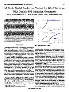
Fig. 2. Ar.Drone 2 quadcopter and its reference axes (black - global axis; red - rigid body axis).
empc = mpc.toExplicit() Finally the binary search is costructed tree = BinTreePolyUnion(empc.optimizer); In order to obtain the point location algorithm based on binary search tree we need to execute export function (a) Flappy bird in action.
(b) Highest score.
toPythonTree(tree,’flappympc’,’primal’) Fig. 1.
Screenshots of the Flappy Bird game.
The generated algorithm was imported into flappympc.py which was imported to the application code.
reference is calculated as a middle point between the upper and lower pipes. Under such assumption the designed MPC controller has the following form
min
N −1 X
kxk − xref k1 ,
The game was not created by us. The Python version of this application could be downloaded from [14]. The author of this application used a special library Pygame [15]. This library is used to create a video games in Python. One of the biggest advantage of these languages it’s they open-soure policy and portability between systems.
(11a)
k=0
−1 s.t. xk+1 = xk + buk − f, ∀k ∈ NN , 0
uk ∈ {0, 1}, ∀k ∈ N0N −1
Import the generated controller into the application was really easy. The condition checking if the button was pressed on keyboard is replaced by an generated point location algorithm based on binary tree approach, which based on the current and desired height can decide if the actual height must be increased or not.
(11b) (11c)
note that in (11c) the input’s binary character is explicitly defined. This kind of optimal control problem can be easily formulated via MPT only in few lines of code.
At the final phase we compared the designed MPC based controller with a human like players. Few candidates were to ask to try control the height of the bird in this application. From Table 1. , which summarizes the results, can be seen that the designed MPC controller’s is diametrically better compared to the human players.
model = LTISystem(’A’,1,’B’,18,’f’,-9) model.u.with(’binary’) model.x.with(’reference’) model.x.reference = ’free’ model.x.penalty = OneNormFunction(1) N = 4 mpc = MPCController(model, N)
TABLE I.
ACHIEVED SCORE IN F LAPPY B IRD
Players 1. Player 2. Player 3. Player MPC
The first line of the code creates an instance of the object LTISystem where the affine dynamic of the system (10) is defined. Afterward the control input values are restricted, it can acquire only binary values (0 or 1). Furthermore we need to have a possibility to change the value of the reference, this is ensured by the fourth line of the code. Finally the penalty matrix is defined as a 1-norm between the actual and desired height. After the model’s parameters are defined and the prediction horizon is set another object is called to create an instance, which will hold the information about defined optimal control problem (11). The explicit representation of control law in (7) is constructed by by the following way:
Average score 16 14 9 182
Best score 33 19 17 473
B. Application 2: Quadrocopter Control In this case study we demonstrate an application of explicit model predictive control on a lowcost quadrocopter [16], pictured in Fig. 2. To keep things simple we present just a regulation of a single output of the quadrocopter (the yaw angle control). The Robot Operating System (ROS) framework [9] was used to implement the explicit mpc. ROS supports various
81
0.6
programming languages like Python or C to carry out control algorithms for the quadrocopter. ROS offers libraries of functions that interface data from quadrocopter’s sensors and actuators. The data from sensors like an electronic compass and an accelerometer are repeatedly acquired 200 times per second and convey by WiFi to PC.
0.5 0.4 uψ˙
0.3 0.2
The quadrocopter’s onboard software executes low level control loops to control the vertical velocity z, ˙ yaw velocity ˙ roll φ and pitch angle θ based on input references. ψ,
0.1 0
The control inputs of the quadrocopter are:
-0.2
•
uz˙ , the vertical velocity reference;
-0.1 0
•
uψ˙ , the z axis rotation velocity reference;
•
uφ , the x axis rotation velocity reference;
•
uθ , the y axis rotation velocity reference.
Fig. 3.
5
Time (s)
10
15
Control input for the Ar.Drone example.
100
All inputs are normalized to −1 ≤ u ≤ 1. In this case study we regulate the yaw angle w.r.t the global axis, as shown in Fig. 2. In the [17] a rough modelling of the quadrocopter’s rotational dynamic over the z axis was given in the form: ˙ ψ¨ = K1 uψ˙ − K2 ψ, (12)
ψ, ψ˙
50
where ψ˙ denotes the angular velocity. The constants K1 ,K2 represent model parameters that need to be identified from an input-output data. K1 uψ˙ denotes a driving torque in z axis, and K2 ψ˙ a drag torque in (12). Using the Euler approximation with (12), gives the approximate discrete-time model: ¸ ¸· ¸ · · ¸ · ψ˙ k+1 = 1 − K2 Ts 0 ψ˙ k + K1 Ts u (13) ψ˙ k 0 Ts 1 ψk ψk+1 |{z} {z } | {z } | {z } u | {z } | xk+1
xk
A
B
k
where Ts denotes the sampling period. To be able to penalize the change of the control input directly we augment the model (13) into the following form · ¸ · ¸ A B B x ˜k+1 = x ˜k + ∆uk , (14) 0 I I | {z } |{z} ˜ A
£
where x ˜k = ψ˙ k
ψ
uk−1
˜ B
¤⊤
.
Utilizing the Multi-Parametric Toolbox we have devised the next MPC problem, objective of which is to bring the yaw angle and the yaw speed to zeros and to reject disturbances: min
N −1 X
x ˜Tk+1 Qx x ˜k+1
+
∆uTk Qu ∆uk ,
(15a)
k=0
˜xk + B∆u ˜ k s.t. x ˜k+1 = A˜ ∆uk = uk − uk−1 , − 0.005 ≤ ∆uk ≤ 0.005, − 1 ≤ uk ≤ 1, " # " # 1000 −1000 −180 ≤ x ˜k ≤ 180 −1 1
(15b) (15c) (15d) (15e) (15f)
82
0
-50
-100 0 Fig. 4.
5
Time (s)
10
15
States of the drone.
The model parameters were identified as K1 = 91.230, K i2 = h 100 0 0 3.814, while the state penalty matrices Qx = 0 2000 0 and 0 0 1 Qu = 1 were chosen experimentally. The cost functions was ˙ The prediction horizon tuned to accent ψ and slightly stifle ψ. N = 5 and control period Ts = 20.0ms were used. The parametric feedback law as in (7) was then computed utilizing parametric solvers included in MPT. The solution comprised 281 regions. The binary tree was generated with 3490 nodes while the depth of the tree was just 15 levels. Next the explicit controller was exported to Python code using the toPython procedure and placed into the operating software within the ROS framework. The explicit mpc was evaluated in a real-time experiment with control period ∼ 20ms. The true control period differed from 16 to 29 milliseconds, which brought additional disturbances into the control. Moreover the processing of sensor data and the controller evaluation was asynchronous due short WiFi drop-outs. To get the most accurate values of ψ and ψ˙ in each period a Kalman observer was developed. The control performance is captured by Figs. 3 and 4. As can be seen, the explicit MPC controller rejects disturbances and achieves ˙ to the regulation objective by bringing both ψ as well as (ψ) zero. The velocity oscillations were caused by changing control period, WiFi drop-outs and air turbulence around quadrocopter.
ACKNOWLEDGMENTS The Authors gratefully acknowledge the contribution of the Slovak Research and Development Agency under the project APVV 0551-11 (APVV SK-FR-0004-11). The authors gratefully acknowledge the contribution of the Scientific Grant Agency of the Slovak Republic under the grants 1/0403/15 and the internal grant of the Slovak University of Technology in Bratislava for support of young researchers. R EFERENCES [1] S. Qin and T. Badgewell, “An overview of industrial model predictive control technology,” Chemical Process Control, vol. 93, no. 316, pp. 232–256, 1997. [2] M. J.M., Predictive Control with Constraints. Prentice-Hall, 2001. [3] A. Bemporad, M. Morari, V. Dua, and E. N. Pistikopoulos, “The explicit linear quadratic regulator for constrained systems,” vol. 38, no. 1, pp. 3–20, Jan. 2002. [4] S. Diamond, E. Chu, and S. Boyd, “CVXPY: A Python-embedded modeling language for convex optimization, version 0.2,” http://cvxpy.org/, May 2014. [5] J. Andersson, “A general-purpose software framework for dynamic optimization,” PhD thesis, Arenberg Doctoral School, KU Leuven, Department of Electrical Engineering (ESAT/SCD) and Optimization in Engineering Center, Kasteelpark Arenberg 10, 3001-Heverlee, Belgium, October 2013. [6] [Online]. Available: https://projects.coin-or.org/Ipopt [7] [Online]. Available: http://www.sbsi-sol-optimize.com/asp/sol product snopt.htm [8] [Online]. Available: http://www.worhp.de [9] M. Quigley, K. Conley, B. Gerkey, J. FAust, T. Foote, J. Leibs, E. Berger, R. Wheeler, and A. Mg, “ROS: an open-source Robot Operating System,” ICRA, vol. 3, no. Figure 1, p. 5, 2009. [Online]. Available: http://pub1.willowgarage.com/∼konolige/cs225B/ docs/quigley-icra2009-ros.pdf [10] M. Herceg, M. Kvasnica, C. Jones, and M. Morari, “Multi-Parametric Toolbox 3.0,” in Proc. of the European Control Conference, Z¨urich, Switzerland, July 17–19 2013, pp. 502–510, http://control.ee.ethz.ch/ ∼mpt. [11] F. Borrelli, Constrained Optimal Control of Linear and Hybrid Systems. Springer-Verlag, 2003, vol. 290. [12] M. Baoti´c, “Optimal Control of Piecewise Affine Systems – a Multiparametric Approach,” Dr. sc. thesis, Zurich, Switzerland, Mar. 2005. [13] P. Tøndel, T. Johansen, and A. Bemporad, “Evaluation of piecewise affine control via binary search tree,” Automatica, vol. 39, no. 5, pp. 945–950, 2003. [14] [Online]. Available: https://github.com/sourabhv/FlappyBirdClone [15] [Online]. Available: http://www.pygame.org [16] P. J. Bristeau, F. Callou, D. Vissi`ere, and N. Petit, “The Navigation and Control technology inside the AR.Drone micro UAV,” in IFAC Proceedings Volumes (IFAC-PapersOnline), vol. 18, no. PART 1, 2011, pp. 1477–1484. [17] J. Engel, J. Sturm, and D. Cremers, “Camera-based navigation of a low-cost quadrocopter,” in IEEE International Conference on Intelligent Robots and Systems, 2012, pp. 2815–2821.
83