Video Stabilization Using Scale-Invariant Features

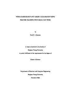
Video Stabilization Using Scale-Invariant Features Rong Hu1 , Rongjie Shi1 , I-fan Shen1 , Wenbin Chen2 1 Department of Computer Science and Engineering, Fudan University 2 Department of Mathematics, Fudan University Handan Road 220, Shanghai, China {052021175, rjshi, ifshen, wbchen}@fudan.edu.cn Abstract Video Stabilization is one of those important video processing techniques to remove the unwanted camera vibration in a video sequence. In this paper, we present a practical method to remove the annoying shaky motion and reconstruct a stabilized video sequence with good visual quality. Here, the scale invariant(SIFT) features, proved to be invariant to image scale and rotation, is applied to estimate the camera motion. The unwanted vibrations are separated from the intentional camera motion with the combination of Gaussian kernel filtering and parabolic fitting. It is demonstrated that our method effectively removes the high frequency ‘noise’ motion, but also minimize the missing area as much as possible. To reconstruct the undefined areas, resulting from motion compensation, we adopt the mosaicing method with Dynamic Programming . The proposed method has been confirmed to be effective over a widely variety of videos.

1. Introduction Video enhancement techniques have attracted great interests in recent years. Hand-held and mobile video cameras become more and more popular in consumer market and industry, due to the decrease in their cost. However, the unsteadiness and unexpected vibrations in video sequences, inherent in these devices, have weakened their performance significantly. In the past decades, numerous researches have been done in the video stabilization field. Its main goal is to remove the unwanted vibrated motion caused by a person holding the camera or mechanical shake, and to synthesis a new image sequence as seen from a new stabilized camera trajectory. There are two kinds of methods proposed to solve this problem: hardware approach and image processing approaches. Hardware approach, or optical stabilization, activates an optical system to adjust camera motion sensors

11th International Conference Information Visualization (IV'07) 0-7695-2900-3/07 $20.00 © 2007

when annoying shaky happened, such as a Steadicam rig or gyroscopic stabilizers. Even though this method potentially works well in practice, it is not broadly chosen due to the cost and the limitation of processing gross motion of the camera. Another method used in stabilization is the image post-processing technique, which is our concern in this paper. In general, the scheme of the digital stabilization includes three aspects: (1) interframe motion estimation; (2) motion smoothing and compensation; (3) filling up the missing image areas. Here, we will follow these steps to describe our method.

1.1. Previous work The development of video stabilization can be traced back to the work of Ratakonda [12], who performed the profile matching and sub-sampling to produce a low resolution video stream in real time. Chang et al. [4] presented an approach to feature tracking based on optical flow, calculating on a fixed grid of points in the video. Buehler et al. [3] proposed a novel approach by applying Image-Based Rendering techniques to video stabilization. The camera motion was estimated by “non-metric” algorithm. Image-Based Rendering was then applied to reconstruct a stabilized video and the smoothed camera motion. This method avoided the problem of stabilization of non-planar scenes and rotational camera motions existing in the homography-based schemes. However,this method only performs well with simple and slow camera motion. A 2.5D motion model was introduced by Jin et al. [7], adding an additional depth parameter to handle videos with large depth variations. However, all of three depth motion models could not simultaneously handle horizontal translation, vertical translation and rotation. Litvin et al. [8] applied the probabilistic methods to estimate intended camera motion. This method produced very accurate results, but it required tuning of camera motion model parameters to match with the type of camera motion in the video. Finally Matsushita et al. [10, 11] developed an improved method for reconstructing undefined re-

gions called Motion Inpainting and it was a practical motion deblurring method. This method produced good results in most cases, but it was strongly relies on the result of global motion estimation. Recently, the use of invariant features for object recognition and matching has increased greatly [1, 2, 9, 13]. Invariant features, found to be more repeatedly and matched more reliably than traditional methods such as Harris corners, are designed to be invariant under the scaling and rotation transformation. In this paper, we use Lowe’s Scale Invariant Feature Transform(SIFT) [9] features to estimate the interframe transformation. Due to the excellent properties, scale invariant features have been widely used in object recognition in the past years, such as the fully automatic construction of panoramas method proposed by Brown and Lowe [2]. Video completion is still a challenge in recent researches. The most widely used approach is Mosaicing [8], blending the neighbor frames to fill up the missing image areas. Unfortunately, significant artifacts might occur when moving objects appear at the boundary of the video frame or the scene is non-planar. Wexler et al. [14] sampled spatio-temporal volume patches from different portions of the same video to repair the holes. However, it cost high computation and requires a long video sequence to increase the chance of finding correct matches. Jia et al. [6] segmented the video into two layers, foreground and background, and repaired the video in these two layers individually. This approach also required a long video sequence, or at least a sequence containing a single motion period of the moving object. Matsushita et al. [10, 11] propagated local motion from defined areas to missing areas, naturally filling up the missing areas even when scene regions were non-planar and dynamic. This method was free from the smearing and tearing present in previous methods. However, it might fail when speedily-moving objects are in the scene, and real-time frame rates are not possible at the current time.

1.2. The proposed method Firstly, a feature based motion estimation method is used. Instead of extracting the common corners or boundaries, which always produce discreditable result, we make use of the scale invariant features [9]. It is demonstrated that these features are affine invariant and nonsensitive to the change of the scale and illuminance. This method have been widely used in the field of image matching and object recognition. As far as we are concerned, it has not been used to solve the video stabilization problem yet. Secondly, Gaussian filtering combined with Parabolic fitting method is applied to estimating intentional motion. Intentional motion, such as zooming the image, panning,


translational or dolly motion with respect to the scene, is slow and smooth compared with unwanted, parasitic camera movements. The stabilized video defined in this paper is close to that mentioned in [10]. The stable motion we expect is not completely motionless, instead only high frequency camera motion is removed. The advantage of our method is that the undefined area caused by motion compensation is as minimized as possible,keeping more information in the video. The comparison will be made in details later. Finally, a new mosaicing method with Dynamic Programming is proposed to fill up the missing area. The idea of using DP method is spurred by [5]. In Davis’s work, a single ‘correct’ frame is used to mosaic the region including the motion object to avoid the discontinuity and blur of focus object. The dividing boundary falling along a path of low intensity in the difference image. This segmenting mosaics method is also useful for the inexact registration resulting from lens distortion or unintentional parallax from image discrepancy. Since it is not required to find a global optimal path in our problem, Dynamic Programming algorithm is more effective than Dijkstra algorithm. The primary contributions of this paper are: • tracking the scale invariant feature transform (SIFT) features to estimate the global motion. • using segmenting mosaics method by Dynamic Programming(DP) to fill up the missing areas in the stabilized frames. To the best of our knowledge, both of these two ideas have not been applied to the video stabilization problem so far. The rest of this paper is organized as follows. Section 2 describes the camera motion estimation based on the scale invariant features. The intentional motion estimation with Gaussian kernel smoothing and parabolic fitting is drawn in Section 3. Section 4 presents the proposed mosaic method using Dynamic Programming. The results of our experiments is shown in Section 5, followed by the conclusion.

2. Motion Estimation The first step of video stabilization algorithm is to estimate the interframe motion. Feature-based approach has been used by the majority of existing stabilization techniques. The most commonly used features in the previous work are image contour or region boundaries, both of which are sensitive to changes in image scale and likely to be disrupted by cluttered backgrounds near object boundaries. In this paper, we estimate the global motion based on the SIFT features instead. Firstly, we will describe the selection of motion model in the following subsection.

2.1. Aﬃne model The geometric transformation between two images can be described by a homography. Estimating a full 3D model of the scene including depth, while desirable, generally results in ill-posed, complex problems that form a field of research on its own. Therefore, in this paper we adopt a six parameter 2D affine motion model, which is commonly used. p = (x, y, 1)T and p = (x , y , 1)T are the pixel locations in the projective coordinates, which respond to the same point in the space. The relationship between these two location can be expressed by p = T × p ; that is,       x a1 a2 a3 x y  = a4 a5 a6 y  . (1) 1 1 0 0 1 The affine matrix T can describe accurately pure rotation, panning, and small translations of the camera in a scene with small relative depth variations and zooming effects. The model translation is (a3, a6) and the affine rotation ,scale ,and stretch are represented by (a1, a2, a4, a5). For most scenes, the conditions are satisfied, and the proper choice of a cost function used in registration can reduce the errors of model mismatch.

2.2. Scale Invariant Feature Transform The selection of feature points in the registration is an essential issue. The features commonly used in the previous work are image contours or region boundaries, and these features move unpredictably with respect to the rest of the image. Therefore, when rotation, scale or change of illumination is taking place, the produced results might be unreliable. Lowe [9] has demonstrated that SIFT features are invariant to images scaling and rotation, and partially invariant to change in illumination and 3D camera viewpoint. Since SIFT features are well localized in both the spatial and frequency domains, the probability of disruption caused by occlusion, clutter, or noise is reduced. Moreover, the features are highly distinctive, which allows a single feature to be correctly matched with high probability against a large database of features. These properties make the matching based on SIFT features more robust and reliable.

2.3. Parameter estimation Several techniques to estimate this interframe transformation have been proposed, such as phase correlation [2] approach and feature tracking [9] approach. In this paper, we adopt the method mentioned in [9] to estimate the parameters of the affine model. Firstly, a fast nearest-neighbor algorithm is applied to match the SIFT features extracted in


above section. Then, clusters belonging to single object is identified with Hough transform. Verification is performed through least-squares solution for consistent motion parameters. The robustness of this approach has been demonstrated.

3. Motion Smoothing The intentional motion in the video is usually slow and smooth, so a stabilized motion can be obtained by removing undesired motion fluctuation, high frequency component in the original video sequence. There is no unified standard to evaluate the smoothness. The goal of video stabilization is producing a visually pleasant video. In our work, we combine two smoothing methods to produce a more acceptable stabilized motion. The one is the similar with the method proposed in [10]. In order to avoid the accumulative error due to the cascade of original and smoothed transformation chain, local displacement among the neighbor frames is smoothed to generate a compensation motion. In this paper, we denote the transform Tij to indicate the coordinate transform from frame i to j. The neighbor frame is denoted as Nt = {m : t − k ≤ m ≤ t + k}. The compensation motion transform can be calculated as, Tti ∗ G(k). (2) Ct = i∈Nt

where G(k) is a Gaussian kernel,and the star mark ∗ means the convolution operator. The motion compensated frame It can be warped from the original frame It by It = Ct It .

(3)

Another method used here is local parabolic fitting. In order to remain the camera’s main motion, a large Gaussian kernel is not appropriate here, which might lead to the problem of over-smoothing(See Figure 1(b)). However, a small Gaussian kernel is not effective to reduce the high frequency camera motion. It is difficult to choose a fit parameter. Here, we add local parabolic fitting to the motion smoothing. As we know, curve fitting method has been broadly used in the stabilization problem. The motion path is controlled by the order of curve and can minimize the undefined regions. Here, the parabola can satisfy the camera motion model. The advantages of such combination are can not only produce smooth moving but also retain the main camera motion path. The result is shown in Figure 1(a). The parabolic fitting is accomplished using the standard least squares method. We denote the parabola as y = ax2 + bx + c , which fits the motion of the video over a window of size N . We can rewrite the pixel coordinates as follows, Az = w,

(4)

15

10

10

5

5 x−translation

x−translation

15

0

0

−5

−5

−10

−10

−15

0

10

20

30

40 time

50

60

70

80

(a)

−15

0

10

20

30

40 time

50

60

70

80

(b)

Figure 1. Motion smoothing results. The images show the changes of x-translation along time in a video sequence. The result of using Gaussian filter together with Parabolic fitting method is shown in (a). According to the order, from outside to inside,the curves describe individually original motion, smoothed motion using Gaussian filter, smoothed motion using Parabolic fitting on the basis of Gaussian filter.(b)is the example of over-smoothing with a large Gaussian kernel.One curve with greater swing describes the original motion, and the other is smoothed motion.

where,the matrix A ,vector x and vector b are   2 x1 x1 1  x22 x2 1  A= . . . . . . . . . . . x2n xn 1 z= a and

w = y1

b y2 . . .

T c yn

(a) Simple Mosaicing Method

T

Since this is an overdetermined system, we can solve for x using the least square solution, z = (AT A)−1 AT w.

(5)

In this paper, we set the parameter of Gaussian filter σ = 2. As we can see, there are still some ‘noise’ motion existing if using a Gaussian filter with a appropriate kernel to remain the main camera motion. As it is mentioned above, this problem can be solved by choosing a better Gaussian kernel, but which causes the motion to be over smoothed. This is not our goal in this paper, see Figure 1(b). However, by combining these two smoothing method, we obtain the stabilized motion curve, and the undefined area is minimized as much as possible. Thus the computation cost of completing the missing areas is reduced.

4. Mosaicing with DP Undefined regions is appeared near the edge of each through the motion compensation. In this paper, we extend


(b) Our Method

Figure 2. Comparison between simple mosaicing method and ours. (a) shows the result of simple mosaicing method. At the bottom, we can see the distinct artifacts and blur. The result using our method is showed in (b). The filled area is satisfied with the defined area in the boundary and there is no blur.

the mosaicing method proposed in [8]. Firstly, we have to find the registration parameters of neighbor frames with respect to the current frame. Given a frame It which has missing area, we need to estimate the transform parameters between frames It and Im where m ∈ Nt . In section 2, we have determined the transform parameters between adjoining frames, which will be used as an initial value. Simply cascading the inter-frame transformation will result in accumulation error and misalignment. Instead, the coordinate transformation can be obtained using cascaded transforms as,

m+1

m+1 m+1 m pm+1 = Tm pm = T m T t pt = T t

pt .

(6)

where the cascaded transformation matrix Ttm and are used as the initial condition. The transformam+1 is estimated by minimizing Energy function (7) tion T t using the gradient descent with only a few iterations. m+1 Tm

E(It , Im , Ttm+1 ) =

(It (pi ) − It (Ttm+1 pi ).

(7)

i∈γ

where γ means all coordinate in the overlapping area between frame It and Im . The contribution of each neighbor frames to the reconstruct missing area can be evaluated as the inverse of registration error E(t, m), Con(t, m) =

1 E(t, m)

(8)

In order to reduce the artifacts in the boundary between the defined and undefined areas, Litvin et al. [8] use additional cross-weighting at the boundary to smooth the transition between the defined area and the mosaic. While we propose using Dynamic Programming to reduce the visual artifacts in the boundary of defined areas and the mosaics. This similar idea is appeared in [5], which solves the mosaicing scene with moving object. The weighting function that decreases near the boundary of a source image will prevent visible discontinuities due to adjustment gain between frames. Although more sophisticated blending functions exist, any function sampling information from all available image produces blurred results in the case of moving objects. We sort the neighbor frames by the contribution calculated above. The frame having the smaller alignment error might have the more probability to be the ‘correct’ source image, used to mosaic the missing regions. When a moving object existing in the boundary of defined region, a single ‘similar’ frame just used to mosaic and hence not leading to blur in the region including the moving object. In our work, we use DP method to find the boundary falling along a path of low intensity in the difference image, leading to minimum visual artifacts in the final mosaic.The results is shown in Figure 2. Blur caused by the weighting function do not happen in our method.

5. Results The performance of the proposed method is evaluated with several video sequences covering different type of scenes. Our experiment is carried out with a Pentium 4 3.0GHz CPU without any hardware acceleration. Except the computation of feature descriptor, the other parts nearly


can be achieved almost in real-time. The number of neighboring frames used in the smoothing motion and mosaicing section is set to be 6*2 = 12. Figure 3 shows the final result of our method, including video stabilization and completion. The fifth, tenth, fifteenth and fiftieth frames of one video are picked up and shown. The top row shows the original frame sequences; the stabilized sequence is shown in the middle row with the missing area. The camera motion becomes slow, but not fixed. The missing area is not very large in our method, which reduces the time used in the completion and the occurrence of artifact. The bottom row shows the mosaicing result with our method. Blur and ghost effects observed by simple frame interpolation method is not yielded here. As we see, the camera motion is stabilized with the robust motion estimation, and the filling areas seem natural.

6. Conclusion In this paper, we propose to estimate the camera motion with SIFT features. These SIFT features have been proved to be affine invariant, and robust in matching across a substantial range of affine distortion, change in 3D viewpoint, addition of noise and change in illumination. Robust motion estimation makes our whole video stabilization stable and effective. In the smoothing step, we extend the local Gaussian smoothing method by parabolic fitting. The stabilized camera motion trajectory is smoother and the missing areas minimized. Instead of using interpolation algorithm to fill up the undefined area, as most simple mosaicing methods do, we propose a mosaicing method with Dynamic Programming. The blur and inconsistency are not yielded in our results. And the whole completion process can be carried out in several seconds for 100 frames. We do not solve the motion deblurring in this paper. The degree of blur in filled area and overlapping area will make the frame unnatural. The high frequency motion inherence in the video needing stabilization also produces motion blur in the original frame sequence. In order to improve the quality, motion deblurring needs to be carried out. In our mosaicing method, the filling pixel can find its value in just one corresponding neighbor frame. This method can effectively decrease the blur produced by blending, but it might causes the temporal inconsistency when objects in the frames have a rapid motion different from the static background. Foreground and background segmentation before warping each frame may benefit the motion deblurring as well as the completion, and it will be added to our work in the future.

References [1] A. Baumberg. Reliable feature matching across widely separated views. Proceedings of the International Conference on

Figure 3. Result of video stabilization. Top row: Original input sequence, and the frame 5,10,15,20 is shown here. Middle row: stabilized sequence which still has missing image areas, and bottom row: stabilized and mosaicing sequences.

[2] [3]

[4]

[5]

[6]

[7]

[8]

Computer Vision and Pattern Recognition, pages 774–781, 2000. M. Brown and D. Lowe. Recognizing panoramas. Proc. International Conf. Computer Vision, pages 1218–1225, 2003. C. Buehler, M. Bosse, and L. McMillian. Non-metric imagebased rendering for video stabilization. CVPR 2001: Computer Vision and Pattern Recognition, 2:609–614, 2001. H.-C. Chang, S.-H. Lai, and K.-R. Lu. A robust and efficient video stabilization algorithm. ICME ’04: International Conference on Multimedia and Expo, 1:29–32, June 2004. J. Davis. Mosaics of scenes with moving objects. Proceedings of IEEE Computer Vision and Pattern Recognition, IEEE Computer Society, pages 354–360, 1998. J. Jia, T. Wu, Y. Tai, and C. Tang. Video repairing: Inference of foreground and background under severe occlusion. Proc. IEEE Conf. Computer Vision and Pattern Recognition, pages 364–371, 2004. J. S. Jin, Z. Zhu, and G. Xu. Digital video sequence stabilization based on 2.5d motion estimation and inertial motion filtering. Real-Time Imaging, 7(4):357–365, August 2001. A. Litvin, J. Konrad, and W. Karl. Probabilistic video stabilization using kalman filtering and mosaicking. Proc. of IS&T/SPIE Symposium on Electronic Imaging, Image and Video Communications, 1:663–674, 2003.


[9] D. G. Lowe. Distinctive image features from scale-invariant keypoints. International Journal of Computer Vision, 60(2):91–110, 2004. [10] Y. Matsushita, X. T. E. Ofek, and H.-Y. Shum. Full-frame video stabilization. Proc. IEEE International Conference on Computer Vision and Pattern Recognition, 1:50–57, June 2005. [11] Y. Matsushita, E. Ofek, W. Ge, X. Tang, and H.-Y. Shum. Full-frame video stabilization with motion inpainting. IEEE Transactions on Pattern Analysis and Machine Intelligence (PAMI), (7):1150–1163, July 2006. [12] K. Ratakonda. Real-time digital video stabilization for multi-media applications. ISCAS ’98: Proceedings of the 1998 IEEE International Symposium on Circuits and Systems, 4:69–72, May 1998. [13] C. Schmid and R. Mohr. Local grayvalue invariants for image retrieval. IEEE Transactions on Pattern Analysis ans Machine Intelligence, 19(5):530–535, May 1997. [14] Y. Wexler, E. Shechtman, and M. Irani. Space-time video completion. Proc. IEEE Conf. Computer Vision and Pattern Recognition, pages 120–127, 2004.