Oct 17, 2001 - In this note, the term data product is used for a small self-contained piece of data. ... approximation of the expected product naming scheme.
CMS NOTE 2001/047
Available on CMS information server
The Compact Muon Solenoid Experiment
CMS Note
Mailing address: CMS CERN, CH-1211 GENEVA 23, Switzerland
October 17, 2001
Views of CMS Event Data: Objects, Files, Collections, Virtual Data Products Koen Holtman1)
Abstract The CMS data grid system will store many types of data maintained by the CMS collaboration. An important type of data is the event data, which is defined in this note as all data that directly represents simulated, raw, or reconstructed CMS physics events. Many views on this data will exist simultaneously. To a CMS physics code implementer this data will appear as C++ objects, to a tape robot operator the data will appear as files. This note identifies different views that can exist, describes each of them, and interrelates them by placing them into a vertical stack. This particular stack integrates several existing architectural structures, and is therefore a plausible basis for further prototyping and architectural work. This document is intended as a contribution to, and as common (terminological) reference material for, the CMS architectural efforts and the Grid projects PPDG, GriPhyN, and the EU DataGrid.
GriPhyN technical report number GRIPHYN 2001-16. This research was supported by the National Science Foundation under contracts PHY-9980044 and ITR-0086044.
1)
Division of Physics, Mathematics and Astronomy, California Institute of Technology
Contents 1 2
3
4
5
Some terminology: objects, events, data products The view stack 2.1 Description of views 1–4 2.2 Description of views 9–5
3
: : : : : : : : : : : : : : : : : : : : : : : : : : : : : : : : : : : : : : : : : : : : : : : : : : : : : : : : : : : : : : : : : : : : : : : : : :
Relation of existing and planned software to the view stack 3.1 Replica catalogs : : : : : : : : : : : : : : : : : : : : : 3.2 Current CMS production : : : : : : : : : : : : : : : : 3.2.1 Multiple mapping routes : : : : : : : : : : : : 3.2.2 No use of the virtual data view : : : : : : : : : 3.3 CMS data grid system of 2003 : : : : : : : : : : : : : : 3.3.1 Mapping from view 2 down to 5 in 2003 : : : : 3.3.2 Other types of data : : : : : : : : : : : : : : :
: : : : : : : : : : : : : : : : : : : : : : : : : : : : : : : : : : : : : : : : : : : : : : : : : : : : : : : : : : : : : : : : : : : : : : : : : : : : : : : : : : : : : : : : : : : : : : : : : : : : : : : : : : : : : : : : : : : : : : : : : : : : : : : : : : : : : : : : : : : : : : : : : : :
Detailed definition of view 3: virtual data product collections 4.1 The CMS data grid system in view 3 : : : : : : : : : : : 4.2 Analysis jobs and request sets : : : : : : : : : : : : : : : 4.3 Quantitative aspects : : : : : : : : : : : : : : : : : : : : Consistency management from an application viewpoint
2
: : : : : : : : : : : : : : : : : : : : : : : : : : : : : : : : : : : : : : : : : : : : : : : : : : : : : : : : : : : :
4 4 5 7 7 7 9 9 9 9 10 11 11 13 13 14
1 Some terminology: objects, events, data products The CMS experiment has an object-oriented software effort and as a result the word ’object’ is heavily overloaded. In some cases, the word ‘object’ is understood to mean ‘a persistent object as defined by the Objectivity/DB database model’. In other cases, one takes the world-view that ‘everything is an object’. In these latter cases, the description of something as being ‘an object’ not say too much about the status of that thing in the data model. To prevent ambiguities, this note avoids using the word ’object’. Instead the terms ‘event’ and ‘data product’ are used, as was done in [1]. These terms are defined as follows.
� Event. In the context of the storage and analysis of CMS detector data, an event is defined as the collision phenomena that occur during a single bunch crossing. An event is not any particular piece of data in a database, rather it is a distinct real world phenomenon that can be measured by the CMS detector, and about which data can be kept in database. In other contexts, in particular in detector simulations, an event can also be a single individual collision during a bunch crossing. � Data Product. In this note, the term data product is used for a small self-contained piece of data. In CMS terminology, as influenced by the Objectivity/DB terminology, data products are often called ‘objects’. The typical size of a data product is 1 KB - 1 MB. A data product is by definition atomic: it is the smallest piece of data that the system can individually handle, or needs to handle. In this note, a data product usually is a piece of data that holds some particular information about a single CMS event. One exception is the ‘parameter data product’ in section 4.1, which holds parameters for a physics algorithm instead. Each event that is represented on storage usually has many data products associated with it, data products which all hold information about that event. However, in this note a data product holding event data is only associated with one single event for which it holds information. Figure 1 illustrates this relation between data products and events. Raw data products for Event 1
RA_1
for Event 2
RA_2
......
......
RB_1
RB_2
Reconstructed data products ESDv1_1
AODv5_1
ESDv2_1 ESDv1_2
TAGV2_1
AODv5_2
AODv7_2
ESDv2_2
TAGV2_2 DPDV3_2
...... The labels like ‘ESDv2_2’ in this picture are only a simplified approximation of the expected product naming scheme.
Figure 1: Different raw and reconstructed data products that exist at some point in time for two events. Each event has a fixed number of raw data products, but a variable number of reconstructed data products. (This figure was reproduced from [1].)
3
2 The view stack The view stack, as introduced in the abstract of this note, is a vertical stack of different viewpoints of the CMS event data in the CMS data grid system. A description of the CMS data grid system can be found in [1]. From top to bottom the stack contains the following views. 1. High-level data views in the minds of physicists 2. High-level data views in physics analysis tools 3. Virtual data product collections 4. Materialized data product collections 5. File sets 6. Logical files 7. Physical files on sites 8. Physical files on storage devices 9. Device-specific file views Figure 2: The view stack, containing 9 different views of the CMS event data in the CMS data grid system. The highest-level view is on top.
2.1 Description of views 1–4 The high-level data views in the minds of physicists are at the top of the stack. In the end, these are the sole purpose of having a CMS data grid system at all. However, this note does not elaborate on these high-level views, as CMS does not currently expect the Grid projects to get involved in the short term in directly supporting the management of such views through research or software [1]. Next are the high-level data views in physics analysis tools, the tools used by the physicists to interact with the CMS data grid system. Many such tools might exist, offering many different views. See [1] for a longer description of these tools, again the Grid projects are not expected to get involved in the short term in building these tools. This note defines the view of virtual data product collections as the highest-level view that is a uniform, common view across the whole CMS collaboration. Section 4 contains an exhaustive description of this view. A short description is as follows. A data product is a small self-contained piece of data, a piece of data that holds some particular information about a single CMS event. The typical size of a data product is 1 KB - 1 MB. A virtual data product is one that doesn’t necessarily have a physically existing representation of its value until this value is requested. A virtual product exists purely because a specification of how to compute its value has been stored in the grid. The act of computing the value of a virtual data product is called the materialization of that product. A virtual data product both has a virtual existence and a virtual location. These two types of virtuality were first defined in [6]. Virtual existence means the physical product value might not exist at all. Virtual location means that, if a physical value does exist, then it can be referenced irrespective of where it is stored. Each virtual data product has a UID (unique identifier) that can be used to obtain the product value from the grid system. A virtual data product collection is a set of virtual data products, usually a set of products that are related in some way that is significant in higher-level views. Such a collection can be defined in full by specifying a set of virtual data product UIDs. The support of a virtual data product collection view in its computing system is a long term goal of the CMS experiment, a goal that has remained surprisingly constant since its initial formulation around 1996 [3]. The exhaustive description of this view that is provided in section 4 is relatively new though, this description was created around February 2001 and is geared towards the Grid projects. CMS does not currently have an implemented API that supports the complete virtual data product collections view in a Grid context. Rather the implemented APIs in the current CMS physics analysis framework [5] should be seen as being one concrete step in an evolutionary 4
development process towards full support of this view. In the short term (from now till 2003, see [1]), the Grid projects are not expected to be involved directly in enhancing the implementation of this virtual data product based, or object based, view. However, long-term Grid research still has to take this view into account, as it is more fundamental to CMS computing than any file based view. The materialized data product collections view is related to the previous view of virtual data product collections. The difference between the two is that the data products in a materialized collection do not have a virtual existence anymore. By definition, if a collection of materialized data products is said to exist in the grid, this implies that all the values of the data products in that collection exist somewhere on storage in the grid. The products still retain their virtual location: the locations where the product values exist are not present in this view, also it is not guaranteed that all these values exist on storage at the same location, and in fact some values might exist on storage in multiple locations. Again, each of the products in a materialized data product collection can be identified by a UID. The CMS physics analysis framework [5] currently implements a basic service for creating, accessing, and manipulating materialized data product collections. In the current framework, collections are referenced by name. The framework supports several types of many-to-many mappings from these collections to the actual (Objectivity/DB database) files containing the product values. The exact many-to-many mapping mechanism that is supported was not specifically designed for the grid. Instead several elements and capabilities of it have arisen almost accidentally as by-products of features of the Objectivity/DB database product. The question of how well the current mechanism is adapted to the grid use case is still very much a research question. At this point it is uncertain how much of the solution we have already.
2.2 Description of views 9–5 The remaining views are best introduced by starting at the bottom of the view stack. Device-specific file views will play a limited role in the grid monitoring and hardware maintenance domain. As an example, in the device-specific view of a file on a tape system, the identity of the tape cartridge which holds the file is visible. In general, grid components will not manipulate files using APIs based on this view. The view of physical files on storage devices is the lowest-level generic view of files. This view is corresponds to the common device-independent file access and manipulation interface that is implemented by the grid components wrapping the actual devices in the CMS data grid system. In this view, many devices exist, and each device contains a set of files. For each device it is known at which grid site this device is located. For each file on a device, estimates of performance characteristics like the file access time can be obtained. The exact definition of this view is coupled to the exact definition of the common storage device interface in the CMS data grid, and this interface does not yet have a fixed, stable definition. The Grid projects, in particular PPDG in collaboration with the EU DataGrid, are still actively designing and developing such a common interface, also the Global Grid Forum (GGF) will likely be involved here. The basic file operations are well understood of course, but other operations expected at this level, like file pinning and obtaining performance estimates, are still in a more conceptual phase. The view of physical files on sites is similar to the previous one except that it abstracts away from file location on specific devices inside a site. In this view, there is a set of grid sites each containing a set of files. If a site S contains a file F , this implies that, in the storage device view, at least one device at site S contains file F . The distinction between this view and the previous one was introduced in [7]. The distinction is motivated by data management issues at large sites which have many distinct storage devices. Such a site might want to move or replicate a file between its storage devices, while at the same time maintaining a fixed site-specific but device-independent file name which it can expose to the outside world. This way the site can move the file internally, without fear of causing global inconsistency, even if the network link to the outside world is down. The view of logical files is a file view where all location information is absent. Logical files simply ‘exist’ in the grid. Logical files will often have some application-specific metadata associated with them. A peculiar property of logical files is that there is no grid API by which one can open and read the contents of a logical file. Instead the model is that the grid may contain several physical files which are known to be representations of the logical file. To operate on the ‘contents’ of a logical file, an API has to be invoked which maps the logical file to one of the physical files that represents it, and then this physical file can then be opened. In the case of read-only logical files, this indirect way of doing things has no big implications, even if the logical file has many physical files that represent it. However, in the case of read/write logical files, write operations will cause the physical files to go out of sync at least temporarily, and this leads to the need to define consistency models and policies which specify the exact allowed write operations, and the semantic relationship between the logical file, its metadata, and its associated physical file contents. 5
The concepts of logical and physical files are strongly related to the Globus replica catalog [8], which implements a service to maintain a mapping from logical to physical files. By design, the Globus replica catalog avoids defining a specific consistency model, instead this model is defined as application-provided and application-specific. This makes the Globus replica catalog implementation more useful to a wider range of applications. However, it also leaves a large semantic gap that has to be filled. Several consistency models with relevance to physics applications were developed in [1] and [10]. Some further points about consistency management are made in section 5 of this note. At the level of abstraction above logical files, there is the view of the grid containing several file sets. The file set concept was introduced in [1] as a generalization of some data handling patterns that are present in the current CMS production effort [4] [5]. A file set is a set of logical files, usually a set of logical files that are related in some way that is significant in higher-level views. This set of logical files is represented as a set of logical file names. A file set can also have some application-specific metadata associated with it. A file set exists by virtue of being registered in a grid-wide file set catalog service. The contents of file sets can overlap: one logical file may be present in many file sets. As with logical files, there is no API to directly open and read the ‘real’ contents or a file set, so there is again a need for consistency models. In fact, the definition of file sets in [1] requires that each file set has a particular consistency management policy registered with it in the file set catalog service. This policy specifies which access and replication operations are allowable on the underlying physical files, if the consistency model of the file set is to be maintained.
6
3 Relation of existing and planned software to the view stack This section relates existing and planned software to the view stack above.
3.1 Replica catalogs Replica catalogs (figure 3) provide mappings between view levels 6,7, and 8. Both GDMP [4] and the Globus Replica Catalog [8] do not make a distinction between a single site and a single storage device, so mapping these to a view level is a bit arbitrary. GDMP can be integrated with a mass storage system (MSS) backend, which takes care of staging files from tape to disk. At both CERN and Fermilab there are GDMP servers deployed in this way: in that case the files in a single GDMP server can be interpreted as files on a site, rather than sites on a particular storage device. The Globus Replica Catalog with HTTP redirection as proposed in [7] implements a mapping from a logical file to a physical file on a site, and then, using a site-specific catalog, down to a physical file on a storage device. GDMP with MSS backend
6. Logical files
Globus RC with HTTP redirection
7. Physical files on sites
GDMP
Globus RC
Site-specific catalog 8. Physical files on storage devices
Figure 3: Relation with existing file catalog implementations
3.2 Current CMS production Figure 4 shows how various components used in the current CMS production effort provide mappings between view levels. A brief overview and introduction to CMS production can be found in section 6 of [1]. 1. High-level data views in the minds of physicists 2. High-level data views in physics analysis tools CMS production web site
3. Virtual data product collections 4. Materialized data product collections 5. File sets
ORCA/CARF+Objectivity tool when reading data GDMP and GDMP with MSS backend
CMSIM simulation tool or ORCA/CARF+Objectivity simulation tool when creating new simulated data ORCA/CARF+Objectivity tool, using extended AMS server, when reading data
6. Logical files 7. Physical files on sites 8. Physical files on storage devices
Extended AMS server
9. Device-specific file views
Figure 4: Relation with the components used in current CMS production In terms of views, production proceeds roughly as follows. First, some physicist in CMS decide that they need a new dataset of simulated CMS physics events, a set with certain properties. They communicate this request to the CMS production team. This request will then be registered in the ‘CMS production web site’ [9]. This web site is not just a set of HTML pages, it is really a specialized database with a web front-end, and we call it ‘web site’ for lack of a better term. After registration in the CMS production web site, and the requested dataset will have a new unique dataset name associated with it (for example eg ele pt30 eta17). The production web site will also have (references to) all information needed to create this dataset. This information takes the form of input parameters to the CMS simulation codes, also sometimes including references to specialized versions of some codes which are needed. The web site therefore maintains a mapping from the dataset name (an identifier for a view at level 1) to a view at level 2, a view in terms of the CMS simulation tools which produce the data.
7
Then a simulation tool can be run to create the data. First the site has to be chosen where the tool will actually be run: this choice is currently done ‘by hand’. Then the tool input parameters taken from the production web site are extended with the necessary site specific parameters like the filesystem location on which the output is to be written. This preparation of the full site-specific set of input parameters for a run of a tool is still partially done by hand, but it is in the process of being fully automated. There are two simulation tools, taking care of different parts of a full simulation chain: the first is CMSIM which is Fortran based and the second is the C++ based ORCA/CARF tool which is integrated with the Objectivity/DB database system. CMSIM will be replaced in future with a more modern tool similar to ORCA/CARF [1]. In terms of view manipulation, it can be said that both current simulation tools map a view at level 2, their input parameters, to views at both level 4 and at level 8. At view level 8, these tools create (or append to) files on particular storage devices. The file names and locations are encoded as part of the tool input parameters. At view level 4 however, the tools output collections of materialized data products, and these collections can be navigated later on when reading the simulation output. For CMSIM output, the mapping between the materialized data product collection view and file view is very direct: one file contains exactly one collection, and file name is also used as the collection name. For the output of ORCA/CARF+Objectivity, the mapping is much more complex. The name of the ‘output collection’ is specified as an input parameter when running the tool, and the output file names are generated according to some logical scheme that embeds this collection name into each generated file name. Multiple instances of the ORCA/CARF tool, running concurrently at the same site, can be writing at the same time to the same output collection and the same output files. The current writing scheme tries to ‘fill up’ output files to sizes just below 2 GB before creating additional files. This strategy of filling up files is used mainly to cope with a constraint of the currently deployed version of the underlying Objectivity/DB database system. This version makes it very painful to have more than 64K different database files in the production effort, so the goal is keep this number below 64K. Newer versions of Objectivity/DB have facilities to ease some of the pain of having more than 64K different database files, but there is no time-frame yet on a switch to using these newer facilities in the CMS production effort. In the longer term however we can expect a lowering of the pressure to fill up files to near 2 GB, which should be good for scalability and manageability of the production effort, as it allows for a greater decoupling between the different running instances of the ORCA/CARF tool. In ORCA/CARF, an example of collection name at level 4 is /System/SimHits/h115gg/h115gg. The actual mapping from such a collection name to a set of physical files is maintained by creating or updating metadata structures in two places. First there is metadata in an Objectivity/DB ‘federation catalog’ file, second there is metadata in an ORCA/CARF ’.META.’ database files. When a collection is moved or copied elsewhere, it is not sufficient to just move the database files holding the materialized data product values: to make the collection accessible one also has to replicate the mapping metadata, replicate parts of the one has to replicate data from the federation catalog file, and some of the ’.META.’ files. Many ORCA/CARF runs will need two input collections, a ‘signal’ and a ‘pileup’ collection, which both have to be present at the same site. At some point after new data has been created for a particular production request, the production web site will be updated to record relevant information like the new request status, output file names, and the current location of these files. In the end, when the whole requested data set has been created, the production web site contains mappings from the data set name to multiple views of the created data, views at (roughly) levels 4 to 7. In addition, the GDMP system records the mapping from view level 6 (logical file name) on the data to views 7 and 8. Reading of production data proceeds as follows. First, the production site is used to discover the name of the production dataset that is needed. Then the this name is mapped to the set of files that are needed. These files will already be at a suitable site, or else the file set can be supplied to a GDMP command which copies the files to a selected suitable site. The GDMP system will also take care of updating an Objectivity/DB federation catalog file at that site in such a way that an ORCA/CARF instance running at that site can map the appropriate collection name at level 4 to the appropriate physical files at level 8. After that, ORCA/CARF can be run at the site, with the collection name as an input parameter. Some large sites will not run a plain version of ORCA/CARF+Objectivity, but a version that uses an ‘extended AMS server’. This extended server implements a mapping between files on the site and files on specific devices, and also often provides integration with a mass storage system, allowing the site greater flexibility in moving files between devices.
8
3.2.1 Multiple mapping routes Figure 5 shows that in CMS production there can be alternative routes when mapping from level 1 down to 8. One route is to go via the production web from 1 to 6, then via GDMP to level 8. Another route is to go via the web site from 1 to 4, then with ORCA/CARF+Objectivity to level 8. The former route is used when moving data around in the grid, the latter is used when invoking actual physics codes once all data needed by these codes is on a single site. The existence of multiple routes to map between views has many consequences. To keep the production effort manageable, it is of course essential that the alternative routes yield the same result. This means that the different stored representations of the different mappings need to synchronized with each other when data is added, copied, or moved. Strategies for this re-synchronization have been grown as the production efforts became more distributed, but as the time of writing this re-synchronization is still a task that relies to a large extent on the knowledge and common sense of the production managers ensure that everything goes right. This reliance on human supervision is of course an impediment to the scalability of the production effort, scalability both in the plain size of the hardware used and in the number of mapping update operations that can be supported. An effort is currently underway add more automation in this area, by formalizing the manual practices that have been developed. In the longer term it is expected that tools and expertise from the Grid projects will play a role in increasing the level of automation, robustness, and scalability. 3.2.2 No use of the virtual data view The current CMS production setup does not use the virtual data product view at level 3. Instead one maps directly from a description of how to materialize data, at level 2, to a materialized data product collection at level 4.
3.3 CMS data grid system of 2003 Figure 5 shows the relation between the view levels and several software components in the CMS data grid system of 2003 as described in [1]. See [1] for a more detailed description of the roles of these components. Comparing the left hand side of figure 5 with the left hand side of figure 4, the production web site and GDMP have now been replaced with 4 components. On the right hand side of these figures, the ORCA/CARF+Objectivity components have been generalized into the ‘CMS framework and object persistency layer’. The CMS file catalog component on the right in figure 5 generalizes the management issues surrounding the Objectivity/DB federation catalog files on the different sites. 1. High-level data views in the minds of physicists 2. High-level data views in physics analysis tools
Physics analysis tools CMS grid job decomposition
3. Virtual data product collections 4. Materialized data product collections 5. File sets
File set catalog Logical file -> physical file catalog
CMS framework and object persistency layer, writing CMS framework and object persistency layer, reading
6. Logical files
CMS file catalog
7. Physical files on sites 8. Physical files on storage devices 9. Device-specific file views
Figure 5: Relation with the software components in the CMS data grid system of 2003 [1] 3.3.1 Mapping from view 2 down to 5 in 2003 According to [1], in the CMS data grid system of 2003, as a baseline the mappings from level 2 down to 5 are all implemented by CMS-provided software components. Nevertheless, in the context of the Grid projects it is 9
useful to consider how these mappings are expected to work. For example, the mapping mechanisms above the file level have an impact on the properties of the file based grid system workload as seen at lower levels. Also, these mappings are relevant to the longer-term research efforts in the grid projects. The mapping from level 2 to 3 is expected to be tool-dependent, and will be performed by various physics analysis tools. The mapping from level 3 to 4 will be done by job planning components in the grid system, components which translate jobs expressed at level 3, as jobs on virtual data product collections, to jobs at level 4, on materialized data product collections. Section 4.2 describes the virtual data product ‘request sets’ of jobs at level 3 in more detail. The execution of a job with a request set R of virtual data products will always involve obtaining the materialized values of all these data products. However this is not necessarily done by creating a set M of materialized data products with M = materialized(S ). Instead the job planning components can suffice with obtaining materialized data product collections M1 ;. . . ; Mn so that materialized(S ) � M1 [ : : : [ Mn . For obtaining each Mi there are three options: 1. find set Mi among the sets of materialized data products that are already stored in the grid, 2. compute (materialize) Mi from scratch, by inserting the necessary subjobs into the concrete job description that is being created, 3. create Mi from other already-stored collections of materialized data products by inserting a subjob that runs a data extraction tool. As a baseline for the 2003 CMS data grid system, a CMS-written component will do the above job planning, though not necessarily in a very optimal way. In the longer term, the Grid projects can make R&D contributions here. The mapping from level 4 to 5 is expected to be a one-to-one mapping: one set of materialized data products is expected to map to one file set. However, one single product in a materialized data product collection might not have a mapping to a single file in the file set. It is possible that the representation of a single product might be scattered over multiple files in the set. Whether this scattering will actually occur depends on the implementation of the CMS ‘object persistency layer’. With respect to the mapping from level 4 to 5, it is also important to note that the contents of file sets may overlap. It is possible that two file sets both contain the same logical file. In terms of view level 4, this means that the contents of two different collections of materialized data products might share some physical storage space. This will in fact be a common occurrence: it is expected that a huge job, in which say a 50 TB collection of data products is to be materialized, will be parallelized by the job planner into smaller subjobs, say 50 subjobs which each materialize a 1 TB collection, followed by a subjob which merges, by reference, these 50 collections into a single collection of 50 TB. It is expected that even after this merging operation, the 50 smaller collections and their underlying file sets will continue to be registered in the catalogs, as this information will likely be useful when optimizing the parallelization of future jobs which use (parts of) these collections as input data. 3.3.2 Other types of data Materialized data product collections, with each data product representing part of a CMS event, are not the only type of data that is stored and transported in the CMS virtual data grid system. Other types of data, like ‘calibration data’ and ‘slow control data’, will also be stored in file sets. These types will have their own high-level view models, and their own mappings into the file set level.
10
4 Detailed definition of view 3: virtual data product collections This section gives an exhaustive description of the view 3 of virtual data product collections. This is the highest view level that represents a uniform, common view across the whole CMS collaboration. The view was first formulated around 1996 [3], but its description here, geared towards the grid projects, is relatively new. Besides virtual data products, the view also contains entities like ‘uploaded data products’ and ‘algorithms’, these are also introduced below.
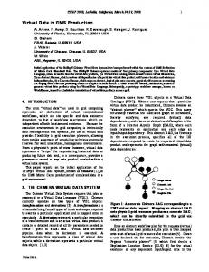
4.1 The CMS data grid system in view 3 Figure 6 shows the structure of the CMS data grid system when seen from the virtual data product collections view. A(PA1,LP1,RA_1,RB_1)
Data grid boundary PA1 RA_1 RB_1 t=0
t=10
t=18
CMS detector
RA_2 RB_2 RA_3 RB_3
LP1
PA2
B(PA2,A(PA1,LP1,RA_1,RB_1))
PA9 B
A G
Job 1
B A G B A
Storage and physics analysis systems outside the data grid
Job 6
G
t=30
= Data flow = Uploaded data product = Virtual data product = Algorithm or job
RA_4 RB_4
Raw uploaded data products
Physicists (users)
B A G ESD virtual data products
AOD virtual data products
New algorithms, parameters, jobs
Figure 6: CMS data grid structure in the virtual data products collections view The data model of this view contains four types of entities: uploaded data products, virtual data products, algorithms, and analysis jobs. A data product is a self-contained piece of data with typically a size of 1 KB to 1 MB. A data product is by definition atomic: it is the smallest piece of data that the system can individually handle, or needs to handle. See [1] for a longer introduction to data products and their use in CMS. In view 3 there are two types of data products: uploaded and virtual. An uploaded data product is one that was generated externally and then uploaded into the grid. In an uploading operation, the value of the data product is transferred into the grid, and a unique identifier (UID) is assigned to the product. The UID (Unique IDentifier) is a label that uniquely identifies an uploaded data product, virtual data product, or algorithm. For uploaded data products and algorithms, these UIDs are generated on the fly, whenever a new product is uploaded or new algorithm is added to the grid. The UID is generated either by the data grid itself or by software outside it. It is not required that these UIDs are short or meaningful to humans: users of physics analysis software should never have to handle these UIDs directly, software components outside the data grid, operating at higher view levels, use metadata to connect these UIDs to higher-level human-understandable concepts. Examples of UIDs in Figure 6 are RA 1, A, B and P A1. The grid is responsible for safely and perpetually storing the values of all uploaded data products. To keep the versioning issues in this data model simple, uploaded data product values are read-only and can never be changed. New or updated values can enter the grid as new uploaded data products, and these always get new UIDs. Some types of uploaded products, those that represent the output of simulation programs, could be deleted from the grid after some time, in order to recycle tertiary storage space. Over time, as shown on the left of figure 6, the CMS detector measures the raw data for different subsequent events. For each event a set of raw data products is uploaded into the grid. The figure shows two products RA i and RB i for each event i. This i is the event ID, a compact identifier that uniquely identifies the event. In practice the raw data for one event will probably be partitioned into some 5–20 products. Partitioning is done according to
11
some predefined scheme that follows the physical layout of the detector. Several subdetector slices will be defined and mapped to products, with each product containing the measurements of all sensitive detection elements in a single subdetector slice. An algorithm is a piece of executable code that computes the value of a virtual data product. Algorithms also get UIDs. Versioning of algorithms during development happens outside the grid system, and the same UID is never used for two different versions of algorithms. An algorithm can take data products as input. In this data model, every algorithm also takes at least one parameter as input, these parameters influence the functioning of the algorithm. The parameters are all modeled uploaded data products. This is modeling as uploaded data products is mainly done for simplicity: a richer data model could also contain parameters which are virtual data products themselves, but such a richer structure is not modeled here, to avoid having to go into detail about the mechanisms that generate the parameter values. There are two types of parameter. Normal parameters are uploaded data products of a size of a few KB, examples in figure 6 are P A1 and P A2. Large parameters are uploaded data products in the MB–TB size range. An example in figure 6 is LP 1. These large parameter data products encapsulate all large data volumes which do not fit easily in the event-by-event data flow scheme of figure 6. Examples of such large parameter data products in CMS are a version of the detector geometry, a version of a calibration dataset, and a set of simulated pileup events1) . If an algorithm inside a CMS executable needs a large parameter value, the algorithm will on average, per event, only read a small part of the parameter value. Which part is read is generally not visible beforehand to the grid components. An algorithm that has a large parameter value as input will therefore have to run in a location that has the whole large parameter value available on local storage, so that fast ‘random’ access to the value is possible. In this data model, the output of an algorithm is uniquely (and deterministically) determined by: 1) the UID of the algorithm, and 2) the values of the data products (including parameters) that serve as input and 3) the platform on which the algorithm is run. The platform is the combination of hardware, OS, compiler, libraries, etc. used to execute the algorithm. Platform differences may result in small, but for the physicist sometimes significant, deviations in the output. The CMS data grid will therefore have to include some facilities to handle platform differences. For the identification of virtual data products, this data model combines algorithm, parameter, and other uploaded data product UIDs in a function notation. Some examples in figure 6 are the virtual data product UIDs A(P A1; LP 1; RA 1; RB 1) and B (P A2; A(P A1; RA 1; RB 1)). In the CMS data flow model inside the grid boundaries of figure 6, there are never two ‘alternative routes’ to a single product, routes in which different algorithms or parameters are used to compute what is conceptually the same product value. Therefore, the function notation in the product UIDs ensures that every single CMS virtual data product has a single UID only. The UID of a materialized virtual data product encodes exactly which algorithms and parameters were used to materialize it, but does not encode any information on the platforms used. We therefore introduce the concept of a platform-annotated UID, which is a virtual data product UID in which each algorithm is annotated with the identifier pi of the platform on which the algorithm was run, or needs to be run. An example is Bp5 (P A2; Ap7 (P A1; LP 1; RA 1; RB 1)). If two virtual data product values have the same platform-annotated UID, they are guaranteed to be byte-wise equal. In figure 6, the virtual data products obtained directly from raw data are generally called ESD (event summary data) products by CMS physicists, those obtained from ESD products are generally called AOD (analysis object data) products. Arrangements of algorithms more complicated than this 2-stage chain are also possible, tough there are no standard acronyms for the intermediate products in such more complicated arrangements. No matter how complicated the arrangement, there is always a strong separation between events: virtual data products can always be traced back to the raw data products of a single event only. Data for different events is only combined inside analysis jobs. 1)
A set of simulated pileup events could also be modeled as a set of virtual data product values. In fact this would be more natural than the approach taken here, which is to model it as a single large parameter data product. The approach taken here has the benefit of keeping the data flow inside the grid simple, but on the other hand it fails to expose some scheduling and optimization opportunities. In the data flow model of figure 6, a set of simulated pileup events could be generated by first defining some virtual data products in terms of CMS simulation algorithms, then running a job which requests their values and merges them into a set which is the job output, and finally uploading this set into the grid again as a single data product.
12
4.2 Analysis jobs and request sets At this view level, physicists make use of collections of virtual and/or uploaded data products by submitting analysis jobs to the CMS data grid system. An analysis job consists of a user-supplied piece of analysis code and a specification of a set of data products. The job instructs the grid system to deliver the values of these data products to the job code. In the case of virtual data products, the product values might need to be materialized before they can be delivered. The job code is run inside the grid, under the control of the grid schedulers. The analysis job code is highly parallel: the job decomposition component in the grid system can break up the job into many subjobs which different subjobs receiving different parts of the requested set of data products. See [1] for more information about the job model and about communication between subjobs. The request set of a job is the set of data products of which the values are requested by the job. An example of a request set (for job 1 in Figure 6) is
[e2f1;2g B (P A2; A(P A1; LP 1; RA
e; RB e))
.
Job request sets always have the form
[e2E fP S1 (e) [ : : : [ P Sn (e)g , where E is an event ID set. This E generally corresponds to a sparse subset of the events taken over a very long time interval. Inside the time interval, event selection is essentially random, uncorrelated with time. Though each set E in isolation has the properties of a random subsample, the event ID sets of subsequent jobs submitted by one user, or by a group of users, have important cross-correlations that can be exploited by caching and replication strategies. The terms P S1 (e) : : : P Sn (e) in the above request set are product selectors, functions which take an event number e and map it to a data product UID, with the constraint that all raw data products mentioned in that UID belong to the event e. To reflect platform constraints, a job request set might include platform-annotations in the product UIDs. The shape and encoding of platform constraints is an issue that needs further work. Some jobs will use random event navigation techniques in accessing the data products requested for each event. For example, a job might list in its request set two data products P S1 (e) and P S2 (e) for each event e in its event set, but for a particular event e8 a worker subjob might first read P S1 (e8 ) and then decide on the fly that it does not need to read the much bigger P S2 (e8 ) anymore to produce its output. The job request set of a job with random event navigation will always be a superset of the actual set of data products read. In extreme cases, this superset can be orders of magnitude larger. This over-specification is not necessarily very inefficient: in general random event navigation will only be used by a physicist if it is known that all virtual data product values in the request set are available already in materialized form. Also, to help the grid scheduler, in generally the job will be submitted with hints that estimate the degree of random event navigation used.
4.3 Quantitative aspects Extensive quantitative information related to product sizes and workloads in the virtual data product collections view is available in [1] and [2]. The remainder of this section provides some additional estimates of the complexity of this view, for the year 2007. For every parameter, the first value given is the expected value that needs to be minimally supported for the data grid system to be useful to CMS. The second value, between parenthesis, is the expected value needed to support even very high levels of chaotic use by individual physicists.
� � � � � � � � �
Events (Event IDs) added to the grid: 2 � 109 /year (1011 /year) (Both real and simulated events) Data products uploaded: 1010 /year (1011 /year) Algorithms added to the grid: 500/year (500/day) Parameter data products uploaded to the grid: 1000/year (500/day) Number of algorithms in the chain from a raw data product to a job: 0-5 (0-30) Number of data products that serve as input to an algorithm: 0-10 (0-50) Number of virtual data products defined by uploaded products and algorithms: >> 1015 /year Virtual data products materialized: 4 � 1010 /year (1012 /year) Virtual data products values cached by the grid: 1010 (1011 ) at any point in time
13
5 Consistency management from an application viewpoint In a distributed system like the CMS data grid, it is necessary to relax consistency in order to preserve performance and scalability. However, this does not mean that very weak consistency is desirable or even acceptable in all cases. The relaxed consistency that will exist at some lower view levels needs to be carefully controlled, and cannot be allowed to ‘trickle up’ into higher view levels. At higher level views, no answer is often better than an answer that might be incorrect. In the CMS data grid system, the file set view level plays a particular role in consistency management. The file set operations should be robust: any operation should either succeed under the consistency model of the file set, or fail. Consider the case of a large file set replication operation. Say that the network goes down when the operation is 99% complete, that the only action that remained to be done was to verify that the local replicas were indeed still up-to-date according to the file set consistency model. However, even though a lot of work has been done, the robustness requirement implies that the operation can only report failure to the caller. The failure report might of course include details that can help optimize any future retry decisions to be made by the scheduler. As an alternative to reporting failure, one could choose instead to extend the operation semantics to allow for completion with a ‘partial success’ status code. A sufficiently intelligent caller might be able to make some progress using a partially completed replica. However this assumes too much intelligence and flexibility on behalf of the caller. In practice the caller will be a grid job, with no code inside to deal with imperfect input data. Our ability to imagine complex mechanisms, which use relaxed consistency as a way making progress in spite of resource outages, outstrips our ability to implement and test such mechanisms. The physics application-level programmers, who write the code which calls on grid-level services to maintain data, are always under time pressure. To make the best use of their time, they will take the following baseline approach in designing their code. For any particular type of data, one single consistency model will be selected, and the application-level code will be written to work reliably under this model. If resource outages result in the grid-level components being unable for the moment to offer data management operations which guarantee consistency under this model, the strategy will be to simply have the application-level code wait with further operations until operations with these guarantees become available again. Only in cases in which the system obviously spends too much time waiting will there be interest in implementing advanced strategies for making progress with operations under lower levels of consistency. Compare this to use of the NFS filesystem: it is annoying that your applications freeze up when the NFS server is down, but this is better than an alternative that continues to run the applications with the risk of data corruption. Rewriting all the applications to use more elaborate filesystem interfaces with relaxed consistency models is not considered as an option. For the design of grid components that maintain data, this implies the following. It will not be very useful to create a grid service that supports an elaborate sliding scale of consistency models for the data it contains, by way of graceful degradation during outages. There will not be enough software manpower to exploit all the various options which are offered. Rather, a grid component which maintains data should have a simple, well-defined and well-documented consistency model for its data, with operations that are robust in spite of outages. A tradeoff has to be made, for each such service, between offering a very strong type of data consistency, which makes coding against the service easier, and supporting a more relaxed type, which will allow for a greater service availability in the face of the expected probabilities for resource outage. Clearly it will be non-trivial to make these tradeoffs, as they rely on quantifying the probabilities.
14
References [1] Koen Holtman, on behalf of the CMS collaboration. CMS data grid system Overview and Requirements. CMS Note 2001/037. http://kholtman.home.cern.ch/kholtman/cmsreqs.ps , .pdf [2] Koen Holtman. HEPGRID2001: A Model of a Virtual Data Grid Application. Proc. of HPCN Europe 2001, Amsterdam, p. 711-720, Springer LNCS 2110. CMS Conference Report 2001/006. Web site: http://kholtman.home.cern.ch/kholtman/hepgrid2001/ [3] CMS collaboration. CMS Computing Technical Proposal. CERN/LHCC 96-45. December 1996. [4] Asad Samar, Heinz Stockinger. Grid Data Management Pilot (GDMP): A Tool for Wide Area Replication. IASTED International Conference on Applied Informatics (AI2001), Innsbruck, Austria, February 19-22, 2001. [5] http://cmsdoc.cern.ch/orca/ [6] I. Foster, C. Kesselman. A Data Grid Reference Architecture - Draft of February 1, 2001. GriPhyN note 2001-12. Available at http://www.griphyn.org/documents/document server/technical reports.cgi [7] http://www.cern.ch/hst/HTTP/ [8] http://www.globus.org/datagrid/replica-catalog.html [9] http://cmsdoc.cern.ch/cms/production/www/html/general/index.html [10] Dirk D¨ullmann, Wolfgang Hoschek, Javier Jean-Martinez, Asad Samar, Heinz Stockinger, Kurt Stockinger. Models for Replica Synchronisation and Consistency in a Data Grid, 10th IEEE Symposium on High Performance and Distributed Computing (HPDC2001) , San Francisco, CA, USA, August 7-9, 2001, IEEE Computer Society Press.
15