IEEE TRANSACTIONS ON GEOSCIENCE AND REMOTE SENSING, VOL. 41, NO. 3, MARCH 2003
719
An Alternative Method to Compute the Component Fractions in the Geometrical Optical Model: Visual Computing Method Hong-Bo Su, Ren-Hua Zhang, Xin-Zhai Tang, Xiao-Min Sun, Zhi-Lin Zhu, and Zhao-Liang Li
Abstract—In this letter, a method called visual computing was used to solve angular four-components’ proportions and directional vegetation cover fraction for discrete canopies and continuous row-planted plants. It proved effective to predict the angular characteristics on pixel scale. The method could be an alternative way to classical solution of geometrical optical models. Visual computing method would be effective especially when the canopies’ spatial distribution and shapes were irregular and could not be described statistically. Index Terms—Four components, geometrical optical (GO) model, quantitative remote sensing, visual computing.
I. INTRODUCTION
G
EOMETRICAL optical (GO) modeling applies to canopies with discrete spatial distribution and distinct architecture and is particularly appropriate for quantitative remote sensing of forest canopies [1]. The modeling and observation of land surface bidirectional reflectance distribution functions (BRDFs) has been an area of active research for the past decade [2]. Many fruitful developments have been pursued. Various GO models have been put forward to study the discrete vegetation-covered land. GO models are proved to be efficient tools to retrieve information of canopy architecture from remotely sensed data. Among others, Li and Strahler [3], [4] developed GO models to study the (BRDF of discrete forest canopies with cone and ellipsoid shapes, respectively. The core of their models is mutual shadowing and four components that include bright crown (BC), bright Manuscript received November 7, 2001; revised July 2, 2002. This work was supported in part by the Special Funds for Major State Basic Research Project of China under Grant G2000077900, the Knowledge Innovation Project of IGSNRR, Chinese Academy of Science under Grants CXIOG-E01-04 and CXIOG-E01-06, the National Natural Science Foundation of China (NSFC) under Project 49890330, and the Yucheng Comprehensive Experimental Station, Chinese Academy of Sciences. H.-B. Su is with the Institute of Geographical Sciences and Natural Resources Research, Chinese Academy of Science, Beijing 100101, China and also with the Civil and Environmental Engineering Department, Princeton University, Princeton, NJ 08544 USA (e-mail:
[email protected]). R.-H. Zhang, X.-Z. Tang, X.-M. Sun, and Z.-L. Zhu are with the Institute of Geographical Sciences and Natural Resources Research, Chinese Academy of Sciences, Beijing 100101, China. Z.-L. Li is with Groupe de Recherches en Télédétection et Radiométrie— Remote Sensing and Radiometry Research Group (GRTS), Laboratoire des Sciences de l’Image, de l’Informatique et de la Télédétection (LSIIT) (Centre National de la Recherche Scientifique (CNRS) UMR-7005), 67400 Illkirch, France and also with the Institute of Geographical Sciences and Natural Resources Research, Chinese Academy of Sciences, Beijing 100101, China (e-mail:
[email protected]). Digital Object Identifier 10.1109/TGRS.2003.810207
ground (BG), dark crown (DC), and dark ground (DG). Chen and Leblanc [5] established a four-scale model where canopy architectures at scales larger and smaller than the tree crown are combined together. Although most of the models developed are mainly concerned about visible and near-infrared wavebands, they are also applicable for thermal infrared waveband. Kimes et al. [6], [7] measured multiangle radiometric temperatures of row-crop and the relationship between view angle effects and plant height, row width, row spacing, vertical temperatures, view angle, and other parameters. Generally, GO models use some simple tree crown geometry and statistical spatial distribution to capture angular characteristics of canopies. They are convenient and easy to implement, but are difficult to be applied analytically if the type of spatial distribution of vegetation is different from the common used. Because of the use of analytical expressions for sunlit and shadowed regions, these models assume that all trees are of the same shape; thus they are not applicable to mixed pixels (consisting of trees of many species) [8]. With the development of computation technology, it is feasible to simulate and retrieve the angular characteristics of the three-dimensional (3-D) heterogeneous land surfaces (a mixture of soil and vegetation) using the numerical solving method. Myneni et al. [9] studied the coupled medium of atmosphere and vegetation using numerical solving of radiation transfer equations. Their model could predict angular reflectance very well. However, it could not provide us the proportions of four components that would be helpful to separate the four components from a mixed pixel. Goel and Thompson [8] are developing a BRDF model called Spreading of Photons for Radiation Interception (SPRINT). Their model uses accelerated ray-tracing/Monte Carlo methods and allows a user to control the construction and distribution of trees. The model can output BRDF, albedo, and Fraction of Photosynthetically Available Radiation of a total pixel, but its target is not used to separate the four components from a mixed pixel. The four-component angular fractions have many applications. For example, in order to estimate the sensible heat flux at vegetation-covered land, we need to know the component temperatures in a pixel. We need to know the component fractions in a pixel, to retrieve the component temperatures. In this letter, on the basis of visual computing, we calculate fraction of vegetation cover and the four-component proportions in a pixel for several typical shapes and spatial distributions of canopies and present the method’s generality in implementation. One group of computation results is validated by in situ measurements. In addition, the potential applications of this method are discussed.
0196-2892/03$17.00 © 2003 IEEE
720
IEEE TRANSACTIONS ON GEOSCIENCE AND REMOTE SENSING, VOL. 41, NO. 3, MARCH 2003
II. METHODOLOGY Visualization is a method of computing. It transforms the symbolic into the geometric, enabling researchers to observe their simulations and computations [10]. Visual computing is an emerging discipline of increasing importance [11]. Visualization in scientific computing is getting more and more attention from many people. Especially in relation with the fast increase of computing power, graphic tools are required in many cases for interpreting and presenting the results of various stimulations or for analyzing physical phenomena [12]–[14]. There are many graphic tools developed to aid the implementation of visual computation. A computer graphics programming language called OpenGL is used. Since its introduction in 1992, OpenGL has become the industry’s most widely used and supported two-dimensional and 3-D graphics application programming interface (API). It is convenient to place a light to illuminate all the objects in the field of view (FOV) and to change the view angles freely. The pipeline of image generation is similar to photo taking by a camera. To generate the image of four components, the ground objects were viewed twice after the 3-D models of plants and ground have been constructed. OpenGL supports the geometrical model construction, whereas the generating of shadow has not been supported directly. One of the viewpoints was from the light position (placed in an infinite distance to act as the sun), and another viewpoint was from the location of the sensor. When the two images were produced, we compared the Z-buffers between them and every point in FOV of sensor could be determined whether it was visible or illuminated. If one point on tree canopy was both visible and illuminated, then it was classified as BC. If the point on tree canopy was visible and not illuminated, it was sorted into DC. Similarly, the visible ground was divided into two types: DG and BG. When all the points in FOV of sensor were classified completely, the proportions of four components could be obtained by the following equation: (1) where expresses one of the four components (BC, BG, DC, stand and DG); denotes ’s proportion; , , , and for sun azimuth, sun zenith, view azimuth, and view zenith anis the total number of points classified to gles respectively; category in the FOV of sensor; and is total number of sam, , pling points in FOV. It is obvious that the sum of , and should be unity. Knowing , we can derive the directional vegetation cover fraction using (2) denotes directional vegetation cover fraction where and the view zenith angle . with the view azimuth angle We should notice that is independent on the sun angles and as it should be. In this letter, a trunk beneath tree crown was introduced in the construction of the tree canopies models, but multiscattering light was ignored. Fig. 1 shows the images captured from screen when our program is running. Four components and mutual
(a)
(b)
(c) Fig. 1. Captured images of ellipsoid-shaped canopies in the principal sun-plane with three different spatial distributions. (a) Edge cluster. (b) North– south row. (c) Random. Solar azimuth angle 20 , solar zenith angle 33 , view azimuth angle 20 , and view zenith angle 45 ).
=
=
=0
=
shadows can be clearly separated. As an example, Fig. 1(a)–(c) illustrates, respectively, images of ellipsoid-shaped canopies with edge clustered, north–south row and random distributions. The circles outline the border of FOV. III. RESULTS AND VALIDATION We choose to study a spatial resolution of 20 m, which is between the spatial resolution of ETM ’s pan band and visible band. Because our remote sensing experiment site is located at Yucheng City in northern China and the local time is set as 10:30 A.M., solar azimuth and zenith angle is 20 and 33 . The azimuth angle is defined as follows: east as 0 , south as 90 , west as 180 , and north as 270 . Negative values for view zenith angle means that the observation is in the opposite side of the sun. As an example, Fig. 2 displays the variation of the four-component proportions and directional vegetation cover fraction in function of the view zenith angles on both the principal and perpendicular sun-plane for three types of tree canopies (ellipsoid, cone, and cylinder) with random spatial distribution. The FOV of sensor is about 400m , and 32 trees are planted within this area. The crown of the tree with cone or ellipsoid shape has a maximum radius of 1.0 m and has a height of 2.5 m. The height of trunk is 1.0 m. For the tree of cylinder shape, there is no trunk added in the modeling. In order to make comparison between different geometric shapes, the height of cylinder tree is set to 2.5 m, the same height as other shapes of trees. In each figure,
IEEE TRANSACTIONS ON GEOSCIENCE AND REMOTE SENSING, VOL. 41, NO. 3, MARCH 2003
721
Fig. 2. Angular variation of the component fractions of canopies in random distribution with three different geometric shapes. Ellipsoid: (a1) on the principle plane, (a2) on the perpendicular plane; cone: (b1) on the principle plane, (b2) on the perpendicular plane; cylinder: (c1) on the principle plane, (c2) on the perpendicular plane.
there are five curves. All the figures share one legend on the upper right. Curves of BC, DC, BG, and DG denote components’ proportion of bright crown, dark crown, bright ground, and dark ground, respectively. The curves of DF are directional vegetation cover fraction. To give more details around the solar zenith angle, the angle increment changes from 5 to 1 when the view zenith angle is in the range of 25 to 38 . From Fig. 2, we can notice all the curves are symmetrical when the sensor (observer) is in the perpendicular plane [Fig. 2(a2), (b2), and (c2)], but they become asymmetrical except DF when the sensor is in the principal plane. The BC curve keeps incremental when view zenith angle changes from 50 to 50 , but the curve of DC is on the contrary [i.e., Fig. 2(a1), (b1), and (c1)]. The BG curve increases monotonously while view zenith angle is in the range of 50 to 33 , and it decreases when the angle changes
from 33 to 50 . For cylinder shape, BG and BC change little when view zenith angle varies from 0 to 33 , which results from the flat-top disk. From Fig. 2, we can see that the angular variation of DF is small between cone and ellipsoid shapes, but DF of cylinder shape has a value of 0.12 larger than that of cone and ellipsoid shapes when view zenith angle is at 50 [i.e., Fig. 2(a2), (b2), and (c2)]. In order to study the effects of different spatial distribution, we placed 32 trees in the FOV according to several distributions. One is center cluster, which means all the trees are planted at the central area of the region given that the trees are not overlapped. Another distribution is called edge cluster, where the trees are planted on the four sides of 20-m square. North–south row is a kind of row-planted distribution, and all the trees are planted in several rows with a direction from north to south.
722
IEEE TRANSACTIONS ON GEOSCIENCE AND REMOTE SENSING, VOL. 41, NO. 3, MARCH 2003
Fig. 3. Same as Fig. 2, but for ellipsoid canopies with three different distributions. (a1), (a2) Center cluster. (b1), (b2) Edge cluster. (c1), (c2) North–south row.
Fig. 3 shows the angular characteristics of an ellipsoid shape with different spatial distributions. Combined with Fig. 2(a1) and (a2), we can compare four patterns of distributions here. The DF curves Fig. 3(b1) and (c1) have a maximal difference as much as 0.15, which shows that row-planted vegetation cannot be treated as some other spatial distribution. The BC value difference between Fig. 3(c1) and (c2) at view zenith angle of 33 is 0.2, which will have a significant influence on the total reflectance of a pixel. It shows that view azimuth angle plays a crucial role in the angular characteristic of discrete row-planted vegetation. To see the angular effects of continuous row-planted vegetation (many crops are continuous row planted, i.e., wheat, soybean), we simulate the continuous row plant using a solid box. The row width is 0.4 m; row height is 0.5 m; and the space interval between two rows is 0.8 m. The curves are shown in Fig. 4. We can see that the curves’ difference between various view zenith angles is even larger.
A field experiment was conducted in Yucheng Remote Sensing Experiment Site at 10:42 A.M. on April 28, 1999. Sixty-four balls were placed on a square soil box according to Poisson distribution, and multiangle radiometric temperatures were measured by a thermal camera. Based on the four-components’ proportion computed by the method presented in this letter, we inverted the four-components’ temperatures using the model developed in [15]. Below are equations of computing mixed temperature based on radiation balance in thermal band
(3)
IEEE TRANSACTIONS ON GEOSCIENCE AND REMOTE SENSING, VOL. 41, NO. 3, MARCH 2003
Fig. 4.
723
Components’ angular fractions of continuous row plants for different orientations.
TABLE I COMPARISON OF MEASURED AND INVERTED TEMPERATURES. DESCRIPTION: COMPARISON OF THE FOUR-COMPONENT TEMPERATURES MEASURED BY A THERMAL CAMERA (AGEMA 590) WITH THESE DERIVED BY INVERSION OF THE THERMAL MODEL [5] USING THE FOUR-COMPONENT FRACTIONS GIVEN BY OUR METHOD
where expresses one of the four components (BC, BG, DC, denotes ’s proportion; is the mixed temperaand DG); , , , and stand for the components’ temture; peratures, respectively; and are emissivity of ground and is the radiometric temperature of sky, which canopy; and can be measured by a portable infrared radiometer. If we measured in more than four different angles, least square method can be used to solve the components’ temperatures. Table I shows the measured and inverted temperatures of four components. The error between them was less than 0.5 C. It is difficult to measure directly the four-components’ proportion in FOV of a sensor, therefore the inverting of temperature is used to validate the visual computing method indirectly. IV. CONCLUSION AND DISCUSSION Visual computing method can be used to solve GO models when the canopies’ spatial distribution and shapes were irregular and could not be described statistically. It proved effective to predict the angular characteristics on pixel scale. The
method could be a complementary way to classical solution of GO models. There is still something left to do to improve this method in the near future. For example, light scattering between continuum of vegetation and soil should be considered. Similar situation exists in leaf and branch angle distribution. It does not, however, prevent us from outlining some potential applications of this method: 1) converting directional reflectance to spherical albedo; 2) improving the accuracy of separation of soil and vegetation temperatures from remote sensed data; 3) studying spatial scale effects of heterogeneous land surface (some theoretical analysis in thermal remote sensing had been done by Becker and Li [16]); 4) developing four-components’ model to retrieve land surface fluxes instead of two layer model [17]; 5) deriving and validating kernels for BRDF. ACKNOWLEDGMENT The authors wish to thank X. Li (Beijing Normal University) and S. Liang (University of Maryland) for their encouragements. They are also grateful to the anonymous reviewers for their useful comments, which helped to improve the quality of this letter greatly. The field experiments were conducted in Yucheng Comprehensive Experimental Station, CAS. REFERENCES [1] J. M. Chen, X. Li, T. Nilson, and A. Strahler, “Recent advance in geometrical optical modeling and its applications,” Remote Sens. Rev., vol. 18, pp. 227–262, 2000.
724
IEEE TRANSACTIONS ON GEOSCIENCE AND REMOTE SENSING, VOL. 41, NO. 3, MARCH 2003
[2] S. Liang, A. H. Strahler, M. J. Barnsley, C. C. Borel, S. A. W. Gerstl, D. J. Diner, A. J. Prata, and C. L. Walthall, “Multiangle remote sensing: past, present and future,” Remote Sens. Rev., vol. 18, pp. 83–102, 2000. [3] X. Li and A. H. Strahler, “Geometric-optical modeling of a coniferous forest canopy,” IEEE Trans. Geosci. Remote Sensing, vol. GE-23, pp. 705–720, 1985. , “Geometric-optical bidirectional reflectance modeling of the dis[4] crete crown vegetation canopy effect of crown shape and mutual shadowing,” IEEE Trans. Geosci. Remote Sensing, vol. 30, pp. 276–291, Mar. 1992. [5] J. M. Chen and S. G. Leblanc, “A four-scale bidirectional reflectance model based on canopy architecture,” IEEE Trans. Geosci. Remote Sensing, vol. 35, pp. 1316–1337, Sept. 1997. [6] D. S. Kimes, S. B. Idso, P. J. Pinter, R. J. Regnato, and R. D. Jackson, “View angle effects in the radiometric measurement of plant canopy temperatures,” Remote Sens. Rev., vol. 10, pp. 273–284, 1980. [7] D. S. Kimes and J. A. Kirchner, “Directional radiometric measurements of row-crop temperatures,” Int. J. Remote Sens., vol. 4, pp. 299–311, 1983. [8] N. S. Goel and R. L. Thompson, “A snapshot of canopy reflectance models and a universal model for the radiation regime,” Remote Sens. Rev., vol. 18, pp. 197–225, 2000. [9] R. B. Myneni, G. Asrar, and F. G. Hall, “A three-dimensional radiative transfer model for optical remote sensing of vegetated land surfaces,” Remote Sens. Environ., vol. 41, pp. 105–121, 1992.
[10] B. H. McCormick, T. A. DeFanti, and M. D. Brown, “Visualization in scientific computing,” Comput. Graph., vol. 21, no. 6, pp. 1–13, 1987. [11] M. Gross, Visual Computing: The Integration of Computer Graphics, Visual Perception, and Imaging. Berlin, Germany: Springer-Verlag, 1994. [12] M. Grave, Y. Le Lous, and W. T. Hewitt, Visualization in Scientific Computation. Berlin, Germany: Springer-Verlag, 1994, pp. 20–27. [13] R. S. Wolff and L. Yaeger, Visualization of Natural Phenomena. New York: Springer-Verlag, 1993. [14] H. Yamashita, V. Cingoski, M. Mikami, and K. Kaneda, “Visual computing concept in finite element analysis,” IEEE Trans. Magn., vol. 33, pp. 1982–1985, Mar. 1997. [15] H. B. Su, R. H. Zhang, X. Z. Tang, X. M. Sun, and Z. L. Zhu, “The thermal model for discrete vegetation and its solution on pixel scale using computer graphics,” Sci. China E, vol. 43, pp. 48–54, 2000. [16] F. Becker and Z.-L. Li, “Surface temperature and emissivity at various scales: definition, measurement and related problems,” Remote Sens. Rev., vol. 12, pp. 225–253, 1995. [17] R. H. Zhang, H. B. Su, Z.-L. Li, X. M. Sun, X. Z. Tang, and F. Becker, “The potential information in the temperature difference between shadow and sunlit surfaces and a new way of retrieving the soil moisture,” Sci. China D, vol. 44, pp. 112–123, 2001.