Visual Map Construction Using RGB-D Sensors for Image-Based
Recommend Documents
dating the virtual view without signicant delay. UWB. Ultra-Wide Band. ... Indoor Navigation for Android, Master's thesis, Masaryk Univer- sity. Czech Republic ...
and the vacuum won't bleed off. This causes the car to ... antifreeze into the
connector. Several GM divisions ... checked are the proper coolant level and
proper ...
F aculty of Computer Science, Dalhousie Universit y ... issue faced by many map-building schemes is the ac- ... The pose estimates can be used to collect ac-.
Then we use a graph partitioning method to find subset of nodes. Experiments on real .... same computer vision algorithm as the one that was used to define the ...
different from the views used to build a map. More recent .... points as map building proceeds. ..... The data are captured in 3 different scenes, namely 'desktop',.
to support collaborative construction and evolution of visual domain ... knowledge, getting advantage of visual representations like icons and images to help in.
For instance, an apple may look green at midday ..... Technical report, Eastman Kodak Company - ... CMOS: Facts and fict
and identifying drilling problem using Visual Analytics techniques. It provides results of an elaborated analysis of sensor measurement datasets that contain ...
Oct 28, 2016 - driving performance in qualitatively different ways. Non-intrusive ... or even, distraction detection from specific actions (e.g., phone usage). Additionally, these ..... covering four driving postures: (1) normal driving; (2) respondi
situation and provide an up-to-minute safe-road map to a shelter in a ..... A map information sharing system among refugees in disaster areas, on the basis of.
Oct 28, 2016 - estimated that, in 2013, 1.25 million people were killed on the roads ..... object detection framework, which scans the image with a cascade of ... Many vision-based algorithms for pose estimation have shown good performance when the .
Planar Segmentation of RGBD Images using. Fast Linear Fitting and Markov Chain Monte Carlo. Can Erdogan, Manohar Paluri, Frank Dellaert. School of ...
Feb 26, 2018 - Xiang Zhang 1, Misaki Mizukoshi 1, Hong Zhang 1 ID , Engkong Tan ...... Lu, S.J.; Zong, C.H.; Fan, W.; Yang, M.Y.; Li, J.S.; Chapman, A.R.; Zhu, ...
Feb 26, 2018 - ... H.; Maroy, A.G.; Tarkegne, Y.; William, M. Distribution of DArT, AFLP, .... Lu, S.J.; Zong, C.H.; Fan, W.; Yang, M.Y.; Li, J.S.; Chapman, A.R.; Zhu ...
alkaloid), Ku (early flowering) and moustache pattern on seed coats; were included. Three to 7 molecular markers were identified within 5cM of each of.
Thus, ORB-. VISLAM [17] ... monocular visual-inertial SLAM system, which enables the loop closure ... versatile monocular visual-inertial odometry [19] [20] was.
The MAP sensor is located directly on the intake manifold or connected to it
through a flexible tube. The MAP ..... CITROËN. Berlingo 1.4 Bivalent. Berlingo
1.4 Bivalent Van. Berlingo 1.4 i Bivalent Van. Berlingo ... Xsara 1.8 i 16V, Break,
Coupe.
in mobile robot navigation with path planning. A ... Through an exploration, the robot is able to make an .... mal form, its parameters can be defined as Ppt =.
This paper presents a set of methods by which a learning agent can learn a ..... 3We did not always follow this restriction in the implementation itself. ..... (b) The picture used for the roving-eye experiment is a close-up view of the ... With spat
Lloyd's Register, London, 24th May 2017. Follow us on www.trussitn.eu. Using Truck Sensors for Road Pavement Performance Investigation. F. Perrotta, T. Parry ...
Oct 18, 2013 - at a sampling frequency of 1 MHz using the NI-USB 5133 oscilloscope. For comparison purposes, an accelerometer. (PCB 352C65) located at ...
KeywordsâDistance Measurement, Infrared sensor, Surface properties, Ultrasonic ... In an unknown environment, it is important to know about the nature of .... direction of the IR signal corresponds to the surface normal (α. = 0). 0. 0.5. 1. 1.5. 2
The process of implementing the Skudai online map forms major discussion of this paper. ... To implement an Internet-based GIS, a map server is required as a ..... server offers as an alternative for online mapping and could be used for cheap.
Visual Map Construction Using RGB-D Sensors for Image-Based
Sep 13, 2017 - high localization accuracy is required by indoor navigation systems, for ... monocular SLAM systems [26â29], the 3D structure of the scene and the .... According to existing research, the ORB descriptor is effective and stable ...... Tardos, âORB-. SLAM: a versatile and accurate monocular SLAM system,â IEEE.
Hindawi Journal of Sensors Volume 2017, Article ID 8037607, 18 pages https://doi.org/10.1155/2017/8037607
Research Article Visual Map Construction Using RGB-D Sensors for Image-Based Localization in Indoor Environments Guanyuan Feng,1,2 Lin Ma,1 and Xuezhi Tan1 1
Communication Research Center, Harbin Institute of Technology, Harbin 150080, China Chair of Media Technology, Technical University of Munich, 80333 Munich, Germany
1. Introduction The emergence of wireless communication and the Global Positioning System (GPS) has ignited the idea of Personal Navigation Systems (PNSs). A PNS has the positioning and navigation functions to provide location information to individuals via portable devices. In outdoor environments, GPS sensors are the most common and efficient navigation instruments. For indoor spaces, however, because satellite signals cannot penetrate buildings, a smartphone with a GPS sensor is incapable of providing reliable position services to a pedestrian. Therefore, indoor localization methods that do not depend on satellite signals have become a research hotspot in recent years. In the recent decade, many indoor localization algorithms have been proposed and implemented. Of these algorithms, most have concentrated on radio signal-based methods, making use of radio access networks. These algorithms are mainly based on measuring the distances to access points by means of the angle of arrival (AOA), the time of arrival (TOA), the carrier phase of arrival (POA), or the received signal strength
indicator (RSSI), and so forth [1, 2]. With the increase of WiFi access points deployed in public areas, researchers have put focus on Wi-Fi-based indoor localization [3–5]. However, the localization system based on Wi-Fi signals usually cannot provide users with stable results because moving objects or persons affect the signal strength. In addition, Bluetooth beacons are also used for indoor localization [6–8]. The effective range of Bluetooth signals is approximately 5–10 meters, which leads to frequent beacon switching and results in high power consumption. For Wi-Fi or Bluetooth-based localization systems, expensive infrastructure needs to be installed and maintained. An evident disadvantage of these localization systems is that Wi-Fi hotspots or Bluetooth beacons as anchor points cannot be moved after the initial calibration. Moreover, if high localization accuracy is required by indoor navigation systems, for example, submeter accuracy, Wi-Fi hotspots or Bluetooth beacons must be densely distributed in public areas [9]. However, in some public buildings, such as railway stations and airports, high-density infrastructures are costly and inconvenient to achieve. Due to these problems, an
2 economical and stable indoor localization method is needed to provide users with quality location-based services. The emergence of vision-based methods has made it possible to achieve good performance in indoor localization in an economical and practical way. Therefore, more and more studies have focused on the field of localization and navigation based on visual methods using smartphones [9–17]. Vision-based localization takes advantage of image retrieval to search for the similar geo-tagged database images for a query image, and then the location of the query image can be estimated. In the phase of visual localization, the homography matrix [10] and the epipolar constraint [11] are typically used to calculate the location of the query images based on the positions of the matched database images. Therefore, the performance of the visual localization system depends on the position accuracy of the database images. However, some existing visual localization methods [11–14] put their focus on the pose estimation of the query camera and do not mention the method of pose acquisition for the database cameras. In these methods, the database images and their positions are captured and recorded manually. However, in this manner, the acquisition of the database images and their positions is a heavy burden in the phase of database generation, especially for large-scale indoor spaces. TUMindoor [15] is a representative indoor database automatically created by a mapping trolley for visual location recognition [16, 17]. For the TUMindoor database, data acquisition equipment including cameras and laser scanners is triggered roughly every 1.2 meters, but this manner is inapplicable for handheld RGB-D sensors because the walking distance of the operator is difficult to measure. A practical way to collect the pose of the database camera is by Simultaneous Localization and Mapping (SLAM) technology, which is widely used in the field of robot path planning and indoor 3D reconstruction. In vision-based SLAM, stereo camera pairs or a monocular camera is used to estimate the 3D structure and simultaneously deduce the pose of the cameras [18–21]. In stereo SLAM system [22– 25], the 3D points are triangulated for every stereo pair, and the relative motion of the camera pair is estimated by a 3Dto-3D feature registration. In contrast to stereo SLAM, in monocular SLAM systems [26–29], the 3D structure of the scene and the relative motion of the camera are computed by 2D bearing data. In recent years, with the emergence of consumer-level RGB-D sensors, RGB and depth cameras are utilized cooperatively to build dense 3D maps of indoor environments [30–33]. Compared with previous SLAM methods, RGBD SLAM is able to preserve the full structural features of indoor scenes and present a superior dense 3D map. In RGB-D SLAM systems, the Iterative Closest Point (ICP) [34] algorithm is a typical method to align the sequential point clouds captured by depth sensors. Then, the aligned point clouds are used to estimate the consecutive frame status (the rotation matrix and the translation vector) and generate the 3D map [32]. In addition, joint optimization combining visual feature matching and shape-based registration is employed to improve the accuracy of the 3D map [33]. The advantage of RGB-D SLAM is significant, as it recovers indoor structures
Journal of Sensors adequately and places the visual features at their position in the map. The existing algorithms of RGB-D indoor mapping pay more attention to indoor scene recovery, but fewer of the algorithms focus mainly on the optimization of the RGB-D camera poses. Moreover, hardly any algorithms optimize the indoor 3D map for visual localization. Therefore, in this paper, a novel method of visual map construction is proposed, and on the basis of the visual map, image-based localization is investigated to estimate the location of the query camera. Kinect [35] is a popular sensor that captures visual images along with per-pixel depth information, which has the potential to be used in visual map construction. The visual map is similar to a dense 3D map for indoor environments, but it is improved according to the actual demands on visual localization. In contrast to [15], there is no need to measure the walking distance during the construction of the visual map. The proposed visual map as a database contains three main elements: first, the floor plans recovered from the reconstructed 3D model, second, the database images captured by the visual sensor (database camera) of Kinect, and third, the poses of the camera views in the database. In the process of localization, the database images and the poses of the database camera are used to achieve the estimation of the query camera location. In this paper, a novel construction method of the visual map is proposed based on local and global optimizations. The local optimization takes full advantage of the visual features and depth values to refine the transformation matrix of the RGB-D camera poses. In the global optimization phase, an RGB-D detection method is presented to accurately detect the loop closure, which is beneficial for improving the performance of the graph-based global consistency optimization. Then, on the basis of the visual map, an imagebased localization method under the epipolar constraint is introduced. This is a new idea of the utilization of the indoor dense 3D map in that the user’s location is estimated by the positional relationship between the query camera and the database camera. Compared with the existing databaseassisted localization systems, such as the single view-based [9, 10] or the CBIR-based [15, 16] localization methods relying on the plane-to-plane homography method which requires that the visual features for localization should distribute in a plane, our localization method utilizes the epipolar constraint to associate database camera poses with query camera poses regardless of scene structures. The performance of the proposed localization method depends on the accuracy of the visual map. Therefore, the optimization of the visual map based on the requirements of the localization is necessary and indispensable. The main contribution of this paper can be stated as four aspects: (1) a local optimization method of visual map construction is proposed based on multiple constraints; (2) in the global optimization, an RGB-D-based detection method is presented to accurately determine loop closures; (3) an image-based localization method is introduced, taking advantage of the proposed visual map; and (4) combining the visual map construction and the image-based localization, a novel integrated localization system is obtained, which contains the offline stage of database generation and the online
Journal of Sensors
3 Kinect
Visual map construction
Depth images RGB-D calibration Server
Local optimization
Loop closure detection
Global optimization
RGB images Offline stage Online stage
Query image
Image retrieval
Query camera’s pose estimation
Query camera’s location
Smartphone
Figure 1: The framework of visual map construction and image-based localization system.
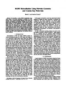
stage of location estimation. The framework of the proposed visual map construction and image-based localization system is shown in Figure 1. The remainder of this paper is organized as follows. Section 2 provides a detailed discussion of the local optimization of the visual map construction. Section 3 describes the loop closure detection algorithm and the global optimization algorithm based on RGB-D images. Section 4 studies the imagebased localization algorithm, including the image retrieval and location estimation of the query camera. Section 5 investigates the performance of the proposed system. Finally, our conclusions are presented in Section 6.
2. Local Optimization Based on MC-ICP for the Visual Map Because the proposed visual localization method is carried out on the visual map, the precision of the visual map determines the localization accuracy to a large extent. Therefore, a multiple constraints ICP (MC-ICP) optimization algorithm is proposed in this paper based on the RGB-D images captured by Kinect. As a local optimization, MC-ICP aligns the RGB image with the corresponding depth image simultaneously captured by Kinect and then minimizes the errors of the point cloud registration in pixel space and 3D space. The ICP algorithm is a conventional and effective method for point cloud registration, but due to the lack of joint optimization by shape and visual information, the transformation between the sequential point clouds hardly achieves the optimum value. Indeed, the ICP algorithm does not utilize data associations provided by the matched visual features in RGB images, and thus the transformation obtained by the classical ICP algorithm inevitably contains errors, which will severely reduce the precision of the visual map and consequently lead to the deterioration of the localization performance. Inspired by this problem, on the basis of the classical ICP alignment, an optimized transformation of the camera poses can be obtained by taking full advantage of the matched visual features and the corresponding depth values. As shown in Figure 2, Kinect has an infrared emitter and two cameras: an RGB camera and an infrared camera. The two cameras are used to simultaneously capture an RGB
Infrared camera RGB camera IR emitter {CC }
{CD }
{CE }
Checkerboard in 3D world
Figure 2: The schematic diagram of Kinect.
image and a depth image in the same scene. The working principle of Kinect is that there is a fixed pattern of speckles generated by the IR emitter projecting onto some object, and after that the speckles on the object are compared with the reference patterns of speckles which have already been stored in Kinect. By this means, the 3D distance between Kinect and the object can be estimated, and then the 3D distance is presented as the disparity image by the infrared camera. Although Kinect is calibrated during manufacturing with a proprietary algorithm, the precision of the manufacturer’s calibration cannot satisfy the requirement of the visual map construction, because the depth distortion is not considered in the manufacturer’s calibration [36]. Therefore, Kinect should be calibrated before the visual map construction to achieve a better accuracy. In this paper, the method proposed in [37] is utilized to calibrate Kinect before the visual map construction. The classical ICP algorithm relies only on the correspondence of the 3D point cloud shapes, which frequently leads to a local optimum and then cannot obtain the rigid body transformation. Therefore, a multiconstraint 3D point registration algorithm is proposed on the basis of the classical ICP algorithm.
4
Journal of Sensors
(a)
(b)
(c)
Y (m)
0
0
0.5 2.5 Z 2 (m 1.5 ) −1
−0.5
0.5 0 X (m)
1
1.5
Y (m)
−0.5
−0.5
0.5 2.8 2.4 Z (m 2 1.6 )
−1
−0.5
(d)
0
0.5 X (m)
1
1.5
(e)
Figure 3: The matched visual features in RGB images and 3D space.
The first step of the proposed algorithm is to match the feature descriptors on the reference image 𝐼𝑟 and the current image 𝐼𝑐 . Here, the reference and current images represent the two successive RGB images in the time domain, and there are also two successive depth images simultaneously captured by Kinect. The most common feature descriptors for image matching are the Scale-Invariant Feature Transform (SIFT) [38] and the Speeded Up Robust Features (SURF) [39]. The ORB descriptor as an efficient alternative to SIFT or SURF is tested to be rotation-invariant and resistant to noise. According to existing research, the ORB descriptor is effective and stable for visual localization [40]. Therefore, in this paper, the ORB descriptors F𝑟 and F𝑐 are extracted from the reference and current images, and because the descriptors are binary, the hamming distance is used to match the descriptors in F𝑟 and F𝑐 . Figure 3(b) shows a result of descriptor matching between the reference image and the current image in an indoor scene as depicted in Figure 3(a). However, Figure 3(b) shows clearly that there are some mismatched pairs between the two feature descriptor sets. To get rid of the outliers, a best fitting transformation matrix is estimated by the Maximum Likelihood Estimation SAmple Consensus (MLESAC) algorithm [41]. The final result of the transformation matrix maps the inliers M𝑟 (M𝑟 ∈ F𝑟 ) on the reference image to the inliers M𝑐 (M𝑐 ∈ F𝑐 ) on the current image, which is shown in Figure 3(c). With this method, one-to-one matching can be obtained between the feature descriptors on the reference image and those on the current image. On the basis of the descriptor matching and the result of the RGB-D camera calibration, there will be two
3D point sets, N𝑟 and N𝑐 , which contain the matched points in the reference point cloud P𝑟 and the matched points in the current point cloud P𝑐 . As an example, the matched 3D points in sets N𝑟 and N𝑐 are separately shown in Figures 3(d) and 3(e) with a 3D view. In contrast to the alignment of images without the requirement of initialization, the alignment of point clouds using the ICP algorithm has shown that if the two point clouds are already nearly aligned, the ICP algorithm can effectively avoid convergence at an incorrect local optimum [34]. Therefore, an initialization method is used before implementing the ICP algorithm by the similar method as Perform RANSAC Alignment proposed in [33]. But, in our initialization method, the RANSAC algorithm is replaced by the MLESAC algorithm, and visual features are described by ORB descriptors instead of SIFT descriptors. The second step of the MC-ICP algorithm is to align the point clouds by the classical ICP algorithm with the initialization result. The ICP algorithm attempts to align two point clouds by means of the nearest local minimum of a mean-square distance metric [34]. Given two 3D point sets, which are the reference point cloud P𝑟 and the current point cloud P𝑐 , the algorithm iteratively strives to obtain TICP using transformation matrix T𝑐,𝑟 by the objective function: TICP = arg min ( T𝑐,𝑟
∑
𝑝𝑖𝑟 ∈P𝑟 ,𝑝𝑖𝑐 ∈P𝑐
𝑟 2 𝑐 𝑝𝑖 − 𝑝𝑖 ⋅ T𝑐,𝑟 ) ,
(1)
where 𝑝𝑖𝑟 and 𝑝𝑖𝑐 are the homogeneous coordinates of the associated points used in the interaction of the ICP algorithm.
Journal of Sensors
5
T𝑐,𝑟 is the transformation matrix that converts the current point coordinates into the reference point coordinates. The transformation matrix T𝑐,𝑟 can be represented as T𝑐,𝑟 = [
R𝑐,𝑟 0 t𝑐,𝑟 1
] ∈ SE3 ,
(2)
where the Euclidean group SE3 contains the rotation matrix R𝑐,𝑟 and the translation vector t𝑐,𝑟 in three-dimensional Euclidean space: SE3 fl {R𝑐,𝑟 , t𝑐,𝑟 | R𝑐,𝑟 ∈ SO3 , t𝑐,𝑟 ∈ R3 } ,
where R𝑐,𝑟 and t𝑐,𝑟 reflect the 3D motion between the current point coordinates and the reference point coordinates. The third step of the MC-ICP algorithm is the optimization procedure of the transformation TICP obtained by the classical ICP algorithm. Because the color and depth features are not taken into account simultaneously, there are not enough constraints for the point cloud registration. The result of the classical ICP-based registration inevitably contains some errors. Therefore, a multiconstraint optimization method is proposed, which optimizes the point cloud registration in both the 3D domain and the image domain. The objective function 𝑓1 and solution T1 can be denoted as 𝑓1 =
algorithm [42], taking TICP as an initial value to achieve solution T1 . On the basis of the above 3D domain optimization, a pixel-level optimization in the image domain is proposed in this paper. The 3D coordinates of the matched descriptors are transformed into 2D coordinates in the image plane, and then the distance of the matched descriptors can be measured at pixel level. The objective function to measure the distance between the matched descriptors at pixel level can be defined as
(4)
+ 𝛼3 (𝑥𝑖𝑐 𝑟13 + 𝑦𝑖𝑐 𝑟23 + 𝑧𝑖𝑐 𝑟33 + 𝑡3 − 𝑧𝑖𝑟 )) ,
𝑓RGB 𝑇𝑐 𝑥 + 𝑢𝑜 − 𝑢𝑖𝑟 ) 𝑧𝑖𝑇𝑐 𝑝𝑥 𝑖
𝑓RGB 𝑇𝑐 + 𝛽2 ( 𝑇𝑐 𝑦 + V𝑜 − V𝑖𝑟 )) , 𝑧𝑖 𝑝𝑦 𝑖
where 𝑓RGB is the focal length of the RGB camera, which is obtained by the RGB camera calibration. The pixel sizes 𝑝𝑥 and 𝑝𝑦 are used to convert the distance in the 3D coordinate system to the image coordinate system. The principle point coordinates (𝑢0 , V0 ) present the intersection position of the principle axis and the image plane. The directional weights 𝛽1 and 𝛽2 , which satisfy 𝛽1 + 𝛽2 = 1, control the contributions of the 𝑋 and 𝑌 directions in the image domain to the overall error. In (7), the 2D coordinates (𝑢𝑖𝑟 , V𝑖𝑟 ) are the position of the matched descriptor on the reference image, and the 3D position (𝑥𝑖𝑇𝑐 , 𝑦𝑖𝑇𝑐 , 𝑧𝑖𝑇𝑐 ) is transformed from 𝑝𝑖𝑐 = (𝑥𝑖𝑐 , 𝑦𝑖𝑐 , 𝑧𝑖𝑐 ) by the transformation matrix T𝑐,𝑟 . Then, the transformed 3D position (𝑥𝑖𝑇𝑐 , 𝑦𝑖𝑇𝑐 , 𝑧𝑖𝑇𝑐 ) can be calculated by 𝑥𝑖𝑇𝑐 = 𝑥𝑖𝑐 𝑟11 + 𝑦𝑖𝑐 𝑟21 + 𝑧𝑖𝑐 𝑟31 + 𝑡1 ,
T1 = arg min (𝑓1 ) ,
𝑦𝑖𝑇𝑐 = 𝑥𝑖𝑐 𝑟12 + 𝑦𝑖𝑐 𝑟22 + 𝑧𝑖𝑐 𝑟32 + 𝑡2 ,
(𝑟𝑖𝑗 ,𝑡𝑘 )
(5) (𝑖 = 1, 2, 3; 𝑗 = 1, 2, 3; 𝑘 = 1, 2, 3) ,
where 𝑛mat is the number of matched feature descriptors; the point 𝑝𝑖𝑐 = (𝑥𝑖𝑐 , 𝑦𝑖𝑐 , 𝑧𝑖𝑐 ) denotes the 3D position of the point in set N𝑐 ; the point 𝑝𝑖𝑟 = (𝑥𝑖𝑟 , 𝑦𝑖𝑟 , 𝑧𝑖𝑟 ) denotes the 3D position of the point in set N𝑟 ; and (𝛼1 , 𝛼2 , 𝛼3 ), which satisfy 𝛼1 +𝛼2 +𝛼3 = 1, are the weights to control the contributions in the 𝑋, 𝑌, and 𝑍 directions. The rotation matrix R𝑐,𝑟 and the translation vector t𝑐,𝑟 as parts of the transformation matrix T𝑐,𝑟 can be described as R𝑐,𝑟
𝑧𝑖𝑇𝑐 = 𝑥𝑖𝑐 𝑟13 + 𝑦𝑖𝑐 𝑟23 + 𝑧𝑖𝑐 𝑟33 + 𝑡3 . To obtain the body transformation, which is constrained in both the 3D domain and the image domain, the optimization should be treated as a multiobjective problem in the two domains. Based on the concept of the Tolerant Lexicographic Method [43] for multiobjective optimization, the solution can be determined as T2 = arg min ( (𝑟𝑖𝑗 ,𝑡𝑘 )
𝑓2 (𝑟𝑖𝑗 , 𝑡𝑘 ) 𝑛mat
),
(𝑖 = 1, 2, 3; 𝑗 = 1, 2, 3; 𝑘 = 1, 2, 3) ,
(6)
t𝑐,𝑟 = [𝑡1 𝑡2 𝑡3 ] . The optimization function shown in (5) can be regarded as a nonlinear least squares problem, where the number of variables is less than the number of matched descriptors. In practical terms, the matched descriptors are much greater in number than the variables in function (4). Therefore, this function can be optimized by the trust-region-reflective
(8)
(9)
(𝑟𝑖𝑗 , 𝑡𝑘 ) ∈ {(𝑟𝑖𝑗 , 𝑡𝑘 ) | 𝑓1 ≤ 𝑓1∗ + 𝜀} ,
where 𝑓1∗ = min(𝑓1 ) denotes the minimum values corresponding to the 3D objective function. For (9), it is a solution for a multiobjective optimization problem that constrains the transformation matrix in both the 3D space domain and the image space domain. This optimization can be treated as a nonlinear least squares problem and solved by the trustregion-reflective algorithm. However, sometimes there is no feasible solution for T2 when 𝑓1 ≤ 𝑓1∗ , and therefore it is
6
Journal of Sensors
(1) F𝑟 ←Extract the ORB feature descriptors from the reference RGB image 𝐼𝑟 ; (2) F𝑐 ←Extract the ORB feature descriptors from the current RGB image 𝐼𝑐 ; (3) Finlier ←Match the feature descriptors in sets F𝑟 and F𝑐 , and exclude the outliers via the MLESAC algorithm; (4) TICP ←Perform the ICP algorithm with the initialization result and the inputs: reference point cloud P𝑟 and current point cloud P𝑐 ; (5) T1 ←Perform 3D domain optimization via the Trust-region-reflective algorithm with the input: TICP ; (6) 𝑓bound = 𝑓1∗ , 𝑖iter = 0; (7) while (𝑖iter ≤ 𝑖max ); (8) (𝑓2 , T2 ) ←Perform pixel-level optimization via the Trust-region-reflective algorithm with the constraint 𝑓bound ; (9) if T2 ≠ Φ (10) The optimization result T∗2 = T2 ; (11) break; (12) else (13) 𝑓bound = 𝑓bound + 𝜀; (14) end (15) 𝑖iter = 𝑖iter + 1; (16) end Algorithm 1: The multiconstraint ICP algorithm.
necessary to expand the constraint by providing a tolerant increment 𝜀 in the process of iterative solving. The detailed process of the proposed MC-ICP algorithm is described in Algorithm 1.
false detection will directly lead to poor performance of the global optimization. Therefore, to precisely detect the loop closure, a novel detection method is proposed based on the RGB-D constraint.
3. Loop Closure Detection and Global Optimization
3.1. Keyframe Selection. Keyframe selection is an essential step of loop closure detection. If the current frame matches all the previous frames the camera has captured, the complexity of the image matching will make the loop closure detection time-consuming. To address the challenge of complexity, keyframes as a subset of the image consequence are introduced, and they contain enough visual features to detect the loop closure. A common way is selecting the keyframe every 𝑛 frames [46, 47] or within a fixed distance interval [48], but some essential visual information in nonkeyframes may be lost in this way. Another feasible way for keyframe detection is based on visual overlap determined by feature matching [49, 50], which is sensitive to object occlusion and image blur. In this paper, the keyframes are selected by two strategies: the fixed-distance strategy and the matching-ratio strategy. A frame sequence is defined as 𝑁 = {𝑛1 , 𝑛2 , . . . , 𝑛𝑙 }, where 𝑛1 is the start frame captured by the RGB camera and 𝑛𝑙 is the current frame. For the fixed-distance strategy, the element in the keyframe set 𝑁1 is selected every 𝑝 frames from the frame sequence 𝑁:
Although the MC-ICP algorithm is proposed as local optimization in the previous section to minimize the errors of the RGB-D alignment, drift caused by the alignment of the associated frames is inevitable, which will ultimately lead to inaccuracies for the visual map, especially for long paths of the camera. Therefore, global optimization is essential to reduce the cumulative errors after the RGB-D alignment. The main process of global optimization can be divided into three parts: keyframe selection, loop closure detection, and graphbased optimization. For loop closure detection, the core task is to find the location that the camera has once visited, and then the path from the previously visited location to the revisited location forms a loop closure. In common research on loop closure, the visual method plays the main role in matching two image frames to determine the loop closure [44, 45]. However, in some cases, the image matching determined by feature descriptors does not definitely mean that the two images were taken in the same location; that is, high similarity of the vision cannot guarantee that the camera is at the same position. Figure 4 shows an example of two images that are matched but that were taken in different locations 1.54 meters apart. In this example, it can be clearly seen that similar images may be taken in different positions while the feature descriptors in the images are matched, so it is unreliable to definitely determine that the camera came back to the previous position. For small-scale indoor environments, the
𝑁1 = {𝑛𝑝𝑞+1 | 𝑛𝑝𝑞+1 ∈ 𝑁, 𝑞 = 0, 1, . . .} .
(10)
However, in practice, the camera controlled by the operator often occurs in a sudden speed increment of the movement, which will lead to the loss of some essential visual information by selecting the keyframes every 𝑝 frames. If the essential visual information is missed, the loop closure detection could fail because there is no previous keyframe matched with the current keyframe. With the purpose of
Journal of Sensors
7
Matched Distanc? = 1.54 m Previously visited location
Revisited location
Figure 4: A false detection of loop closure only by feature descriptor matching.
conserving enough visual information to achieve accurate detection of the loop closure, the matching-ratio strategy is introduced to select the keyframe, ensuring that the keyframes contain sufficient visual features to match with the potential loop closure frame. The matching-ratio selection strategy is proposed on the basis of the fixed-distance strategy to reserve as much visual information between frames as possible. Figure 5 is an illustration of the matching-ratio selection strategy. Between the two successive keyframes 𝑛𝑝𝑞 ∈ 𝑁1 and 𝑛𝑝(𝑞+1) ∈ 𝑁1 , there will be 𝑝 frames that are not selected as the keyframes in the time domain. 𝑛𝑏 is a frame that is not selected by the fixed-distance strategy between 𝑛𝑝𝑞 and 𝑛𝑝(𝑞+1) . Frame 𝑛𝑎 ∈ 𝑁2 denotes a keyframe that has already been selected by the matching-ratio strategy. 𝑁2 is a keyframe set containing the keyframes selected by the matching-ratio strategy. According to the matching-ratio strategy, every frame that does not belong to set 𝑁1 should be separately matched with the nearest previous keyframes selected by the fixed-distance strategy and the matching-ratio strategy. Therefore, frame 𝑛𝑏 should be matched with keyframe 𝑛𝑎 and keyframe 𝑛𝑝𝑞 , separately. This process relies on the ORB descriptor matching as described in Section 3.2, and, after that, the MLESAC algorithm is implemented to exclude the outliers in the matching result. Then, the matching ratios 𝛼1 and 𝛼2 can be calculated by 𝛼𝑖 =
𝑚𝑖 , 𝑚total
(𝑖 = 1, 2) ,
(11)
where 𝑚1 represents the number of matched inliers between 𝑛𝑏 and 𝑛𝑎 , 𝑚2 represents the number of matched inliers between 𝑛𝑏 and 𝑛𝑝𝑞 , and 𝑚total is the total number of ORB descriptors extracted from 𝑛𝑏 . The threshold 𝛼𝑇 is set as a threshold value to verify whether 𝑛𝑏 should be taken as a keyframe and put in set 𝑁2 . The decision rule is that if 𝛼1 < 𝛼𝑇 or 𝛼2 < 𝛼𝑇 , 𝑛𝑏 will be regarded as a keyframe and put in 𝑁2 . Each frame outside the set 𝑁1 will have an estimation as to whether it should be a keyframe for set 𝑁2 , and, after this procedure, the complete keyframe set 𝑁key can be obtained by 𝑁key = 𝑁1 ∪ 𝑁2 .
na
···
npq
···
nb nc
···
np(q+1)
···
Keyframe selected by the fixed-distance strategy Keyframe selected by the matching-ratio strategy Frame outside set N1
Figure 5: An illustration of the keyframe selection by the matchingratio strategy.
It is worth noting that a frame outside of set 𝑁1 is always matched with its two nearest keyframes, which are separately selected by the fixed-distance strategy and the matching-ratio strategy. For example, if 𝑛𝑏 shown in Figure 5 is selected as a keyframe by the matching-ratio strategy, frame 𝑛𝑐 outside of set 𝑁1 next to 𝑛𝑏 will be matched with 𝑛𝑏 and 𝑛𝑝𝑞 . Otherwise, 𝑛𝑐 should be matched with 𝑛𝑎 and 𝑛𝑝𝑞 . In addition, when selecting the first keyframe in set 𝑁2 , a nonkeyframe outside of set 𝑁1 only matches the keyframes in 𝑁1 by (11). 3.2. Loop Closure Detection by the RGB-D Constraint. In general, the keyframe set is large when the camera has a long distance trajectory, and then the keyframe searching is a heavy burden. Therefore, an image retrieval method based on the geographic restriction and bag of features (BOF) [51] is employed in this paper to avoid the global search for the keyframes. In contrast to the general BOF retrieval that searches for similar images in the entire database by the KNearest-Neighbor (KNN) algorithm, the proposed method only searches the keyframes that are within a finite distance. The finite distance will be set depending on the scale of the indoor scene. In this manner, the previous keyframes that are similar to the current keyframe are selected as the candidates to detect the loop closure. For the graph-based global optimization for RGB-D mapping, the performance of the optimization depends on the exact loop closure detection. In the proposed method, the
8
Journal of Sensors
visual and depth data acquired by the RGB-D sensor provide more helpful information to recognize the loop closure more accurately. The main task for the closure detection is to estimate whether the RGB-D camera returns to the position that it has visited before. Therefore, in this paper, the loop closure will be detected by two evaluation criterions: (1) the matching rate of the visual features and (2) the depth consistency of the visual features. The loop closure will be determined only if the current keyframe and the previous keyframe satisfy the two criteria simultaneously. The matching rate of the visual features is proposed based on the vision similarity between the current keyframe and the previous keyframes. The ORB descriptors extracted from the RGB images in the local optimization phase are used to match the current keyframe and the previous keyframes. To reflect the visual similarity clearly between the frames, the matching rate 𝜎mat ∈ [0, 1] is defined as 𝜎mat =
𝑛mat (1/2) (𝑛cur + 𝑛key )
,
(12)
where 𝑛mat is the total number of inliers refined by the MLESAC algorithm. In (12), 𝑛cur and 𝑛key are the number of descriptors extracted from the current keyframe and the keyframes, respectively. In some cases, the matching rate can indicate the positions of the camera; however, there are some exceptions in which the camera captures the same object with different poses, as shown in Figure 4. Therefore, it is necessary to further determine the similarity between the current keyframe and the previous keyframes by the other criterion. In the process of visual feature matching, the ORB descriptors have been extracted and matched between the current keyframe and the previous keyframes. According to the result of the RGB-D camera calibration, each pixel in the RGB image relates to a depth value. For each pair of the matched descriptors in the keyframes, an 𝑟 × 𝑟 pixel patch is defined around the matched descriptor in the keyframes. Then, the depth value 𝑑𝑃 for the pixel patch 𝑃 can be described as 1 𝑑𝑃 = 2 (∑ (𝑑11 + 𝑑12 + ⋅ ⋅ ⋅ + 𝑑𝑠𝑡 )) , 𝑟 𝑠,𝑡
(13)
where 𝑑𝑠𝑡 is the depth value corresponding to the pixel (𝑠, 𝑡) in the patch. Centered on each matched descriptor, a depth value 𝑑𝑃 can be calculated by the depth of the pixel in the patch. If there are 𝑚𝑑 matched descriptors in the current keyframe, there will accordingly be 𝑚𝑑 matched descriptors in the previous keyframe. To measure the distinction of the distance between the object and the camera, an error metric of the depth is defined as 1 ∑ (V𝑐 − V𝑗𝑘 ) , 𝑚𝑑 𝑗 𝑗
(𝑗 = 1, . . . , 𝑚𝑑 ) ,
3.3. Global Optimization by the Graph-Based Method. Due to the errors caused by the camera pose estimation, the path of the camera usually cannot form a globally consistent trajectory. Therefore, the global optimization methods are used to correct the drift introduced by the iterations of the camera pose estimation. The graph-based method for SLAM global optimization is a typical technology to build a consistent map by estimating the parameters associated with vertices (camera poses) in a graph. The g2o framework [52] as an effective graph-based method is employed in this paper to optimize the trajectory of the RGB-D camera estimated by the MC-ICP algorithm. The g2o framework presents the global optimization problem as a graph constraint solved with the nonlinear least squares algorithm. In the framework, the poses of the camera are regarded as the vertices, and the edges serve as the constraints in the graph. For the total of 𝑛pose camera poses in the graph, the error function can be defined as 𝑇
𝑓g2o = ∑ e (k𝑖 , k𝑗 , w𝑖𝑗 ) Ω𝑖𝑗 e (k𝑖 , k𝑗 , w𝑖𝑗 ) , 𝑖,𝑗∈𝑛pose
(14)
where V𝑗𝑐 denotes the depth value of the patch in the current
keyframe and V𝑗𝑘 denotes the depth value of the patch in the
(15)
where k𝑖 and k𝑗 denote the ordered poses of the camera related to the constraint mean matrix w𝑖𝑗 and Ω𝑖𝑗 . Vector e(k𝑖 , k𝑗 , w𝑖𝑗 ) is the error function measuring how well the poses k𝑖 and k𝑗 satisfy the constraint w𝑖𝑗 . According to (15), the optimal trajectory can be described as V∗ = arg min𝑓g2o (V) , V
(𝑠 = 1, . . . , 𝑟, 𝑡 = 1, . . . , 𝑟) ,
𝜎dep =
previous keyframe. The value of 𝜎dep reflects the distinction of the distance between the camera and objects, which also indicates the position difference that the camera shot at. The final decision of the loop closure will be drawn from the two criteria: the matching rate 𝜎mat and the depth distinction 𝜎dep . In practical operation, it is necessary to 𝑇 𝑇 , 𝜎dep ) to determine the loop define a set of thresholds (𝜎mat closure. Only if the current keyframe and the previous 𝑇 𝑇 keyframe satisfy (1) 𝜎mat ≥ 𝜎mat and (2) 𝜎dep ≤ 𝜎dep can the loop closure be ultimately determined.
(16)
where V contains the original camera poses and V∗ contains the optimized poses. The process of the global optimization is described in Algorithm 2. After the global optimization of the camera poses, an integrated visual map constructed by the RGB-D sensor is stored as the database for the visual localization, containing (1) a 3D structure and 2D floor plan of the indoor scene, (2) the database images captured by the RGB-D sensor, and (3) the poses of the database camera. The entire process of the visual map construction is conducted in the offline stage at the service of the online localization.
4. Image-Based Localization Using the Visual Map The image-based localization is an economical and effective method to recognize the position of the user using the
Journal of Sensors
9
(1) 𝑁1 ←Select the keyframes by the fixed-distance strategy; (2) 𝑁2 ←Select the keyframes by the matching-ratio strategy; (3) 𝑁key ←Obtain the keyframe set by 𝑁1 ∪ 𝑁2 ; (4) 𝑡 ←Set the total number of the keyframe set 𝑁key = {𝑛1 , 𝑛2 , . . . , 𝑛𝑡 }; (5) while (𝑡 ≥ 2) (6) 𝜎mat ←Match the current keyframe 𝑛𝑡 with the previous keyframes {𝑛1 , . . . , 𝑛𝑡−1 }; (7) 𝜎dep ←Compute the depth errors of the pixel patches in the current keyframe 𝑛𝑡 and the previous keyframes {𝑛1 , . . . , 𝑛𝑡−1 }; 𝑇 𝑇 and 𝜎dep ≤ 𝜎dep (8) if 𝜎mat ≥ 𝜎mat ∗ (9) V ←Perform the g2o algorithm with the camera pose V; (10) break; (11) end (12) 𝑡 = 𝑡 − 1; (13) end Algorithm 2: Global optimization based on the RGB-D loop closure detection and the g2o algorithm.
query image captured by the smartphone’s camera. This part will focus on the online phase, which is the image-based localization. Taking advantage of the completed visual map, the position of the query camera can be estimated according to the relationship constrained by the epipolar constraint between the query image and the database images. To utilize the epipolar constraint, image retrieval is employed to find the candidate database images that contain the same visual features as the query image. 4.1. Retrieval and Matching between Query and Database Images. In the online stage of the localization, the user captures the query image by the camera equipped on the smartphone, and then the query image is uploaded to the server through the wireless network. In addition, if the smartphone has powerful data processing capabilities, the query image can also be preprocessed on the smartphone, such as the feature descriptor extraction, and, in this way, it is only necessary to upload the data of the feature descriptors to the server. Either way, the visual information captured by the user is the necessary data required by the image-based localization. When the server receives the query image, the ORB descriptors are extracted from the query image. After that, the descriptors are quantized to the visual features, and the occurrences of the features are recorded as a vector to index the query image. For the bag of features, each database image is stored in the bag in the term of the vector related to the occurrence of the visual features. The search engine calculates the similarity between the query vector and the database vector based on the 𝐿 2 distance. In this manner, the most similar database images are selected as the candidate database images using the KNN strategy. The query image retrieval based on the BOF searching is efficient but imprecise and can be regarded as a coarse retrieval. This is because there is no rigid alignment between the query image and the database image using the feature descriptor matching. However, the epipolar constraint acts on the matched descriptors in the images, so it is necessary
to refine the candidate database images obtained by the BOF retrieval. The specific method is that the query image matches each candidate database image using the ORB descriptors, and the outliers are rejected by the MLSAC algorithm. Then, some database images in the candidate set 𝑆can are excluded, since there are few inliers in the matching between the database images and the query image. 4.2. Query Camera Pose Estimation by the Epipolar Constraint. By the retrieval between the query image and database images, the candidate database images are selected according to their visual similarity. In the process of the visual map construction, the poses of the database camera related to the database images are recorded. Therefore, utilizing the query image, the candidate database images, and the poses of the database camera, the location of the query camera can be estimated based on the epipolar constraint. In this paper, the database camera is the RGB camera of the RGB-D device that has been calibrated in the offline stage, and the query camera equipped on the user’s smartphone should be calibrated before the localization. Kdatabase and Kquery denote the database camera calibration matrix and the query camera calibration matrix, respectively. The coordinates Xdatabase and Xquery of the ORB descriptors extracted from the database image and the query image can be normalized by ̂database = K−1 X database Xdatabase , ̂query = K−1 Xquery . X query
(17)
The relations between the normalized coordinates of the ORB descriptors in the query image and the database image can be described as ̂query = 0, ̂database EX X
(18)
where E is the essential matrix, which contains the rotation matrix and the translation vector of the camera transformation. The essential matrix is used to present the camera
10
Journal of Sensors
(1) 𝑆can ←Select the candidate database images by the BOF image retrieval. (2) for 𝑚 = 1 : 𝑘DB (3) E𝑚 ←Compute the essential matrix between the query image and the database image. (4) (R𝐸𝑚 , t𝑚 𝐸 ) ←Decompose the essential matrix E𝑚 into the rotation matrix and the translation vector by SVD. (5) end (6) L𝑖 ←Compute the position of the intersection determined by each two connecting lines. (7) Lquery ←Compute the estimated location of the query camera. Algorithm 3: Image-based localization algorithm.
Object Epipolar plane OQ
ZQ
XQ YQ Query camera
ZD
R E , tE
OD
YD XD Database camera
Figure 6: An illustration of the epipolar constraint.
transformation parameters between the database camera and the query camera in the following form: E ≃ ̂t𝐸 R𝐸 ,
(19)
where ̂t𝐸 denotes the translation vector and R𝐸 denotes the rotation matrix. For t𝐸 = [𝑡𝑥 , 𝑡𝑦 , 𝑡𝑧 ]−1 , ̂t𝐸 is the skewsymmetric matrix of t𝐸 and 0 −𝑡𝑧 𝑡𝑦 [ ] ] ̂t𝐸 = [ [ 𝑡𝑧 0 −𝑡𝑥 ] . [−𝑡𝑦 𝑡𝑥 0 ]
(20) Lquery =
The essential matrix E is determined by the normalized image coordinates of the matched ORB descriptors in the query image and the database image. One efficient method for computing the essential matrix is the five-point algorithm [53]. Via the essential matrix E, the translation vector t𝐸 and rotation matrix R𝐸 can be extracted using Singular Value Decomposition (SVD). The epipolar constraint reflects the pose relationship between the query camera and the database camera, which is shown in Figure 6. By the translation vector t𝐸 and the rotation matrix R𝐸 extracted from the essential matrix E, the 3D position relationship between the query camera and the database camera can be described as X𝑞 = R𝐸 X𝑑 + t𝐸 ,
query camera can be estimated by each pair of the query image and the candidate database image in 𝑆can . However, the estimated 3D position X𝑞 of the query camera obtained by the epipolar constraint is not the definite location, because X𝑞 is always a unit vector. Without a relative scale, X𝑞 cannot indicate the definite distance between the query camera and the database camera, but it contains relative orientation from the database camera coordinate system 𝑂𝐷𝑋𝐷𝑌𝐷𝑍𝐷 to the query database coordinate system 𝑂𝑄𝑋𝑄𝑌𝑄𝑍𝑄. Utilizing a pair of the query image and the candidate database image, the connecting line can be determined based on the known position of the database camera. As shown in Figure 7, for the query image, there are two candidate database images resulting in two connecting lines 𝑙13 and 𝑙23 , and the intersection of the connecting lines is the estimated position of the query camera on the ground plane. Since more than two candidate database images are selected in general, there will be more than two connecting lines that usually cannot intersect one point due to the errors caused by localization. Therefore the average location of intersections is defined as the estimated query camera location Lquery :
(21)
where X𝑞 denotes the 3D position (without the scale) of the query camera and X𝑑 denotes the 3D position of the database camera. Under the epipolar constraint, the position of the
1 𝑛inter
𝑛inter
( ∑ L𝑖 ) , 𝑖=1
(1 ≤ 𝑛inter
𝑘 (𝑘 − 1) ≤ DB DB ), 2
(22)
where 𝑛inter represents the total number of intersections and L𝑖 represents the position of each intersection. The process of the image-based localization is described in Algorithm 3.
5. Simulation Results and Discussion To evaluate the performance of the proposed visual map construction method, an extensive experiment is conducted in our office area as shown in Figure 8. The experimental area includes five offices, two corridors, a classroom, and an exhibition room. These rooms are typical indoor places that have different visual and structural complexities. According to functions and sizes, these rooms are divided into four scene classes, namely, the small room scene (the size is less than 25 square meters, including Office 1 and Office 4), the medium
11
im ag e2
Journal of Sensors
Dat
abas e
Z1
ge y ima Quer
ima ge 1
Y2
Z3 O1
X1 Y1
Y3
O1 Database camera 1
Z3
Da tab as e
Object
O3
O2 X2 O2 Database camera 2
l23
X3
l13 O3 Query camera
Figure 7: The schematic of the image-based localization algorithm. 12.05 m
Office 5
Classroom
3.35 m
5.57 m Corridor 1
Office 4
Office 3
Office 2
Office 1
5.11 m
4.36 m
3.46 m
5.56 m
5.22 m
3.59 m
8.76 m
Corridor 2
Exhibition room
2.89 m
5.98 m
7.41 m
4.81 m
Wall Gate Window
Figure 8: The floor plan of the indoor experimental area.
room scene (the size is between 25 and 40 square meters, including Office 2, Office 3, Office 5, and the exhibition room), the large room scene (the size is more than 40 square meters, including the classroom), and the corridor scene (including Corridor 1 and Corridor 2). Because the implementation of image-based localization relies on the database images and the database camera poses stored in the visual map, the accuracy of the localization is restricted to the precision of the visual map construction, especially for the precision of the estimated database camera positions. To effectively evaluate the precision of the database camera positions, the original trajectory of the RGB-D camera is recorded as the true positions to compare with the estimated positions. For each room or corridor, test points on the camera trajectory are uniformly selected by the step distance of 10 centimeters. The RGB-D camera is moved
sequentially between the test points and placed on a tripod at each test point from the starting location and finally back to the starting location. In order to further explore the influence of different light conditions to the visual map construction, the visual map is constructed both in the daytime and at the nighttime. In the daytime, the lamps in the rooms (with windows) are turned off, but the lamps in the corridors (without windows) are turned on. At the nighttime, all the lamps are turned on, and then the light conditions of the rooms and the corridors are well. The experiment is conducted by Microsoft Kinect v1, and the parameters of Kinect are shown in Table 1. The visual image is captured by the RGB camera on Kinect, and the depth image is simultaneously acquired by the infrared camera on Kinect. All data processing runs on MATLAB 2016B with an Intel Core i5 CPU and an 8 GB RAM.
12
Journal of Sensors
−1.2 −0.6 Y (m)
0 0.6 1.2 1.8 2.4 −4
−2
0
2
4
6
8
X (m) Starting point Original trajectory Estimated trajectory (a)
2.5 2 2 1 0 2.4 1.2
Z (m)
1.5
m)
Y(
0 −1.2
−2
2
0
(b)
4
6
8
)
X (m
1 0.5 0
(c)
Figure 9: An example of the visual map construction in Corridor 1.
Table 1: Parameters of Kinect v1. Variable
Value [unit]
𝑓RGB
4.884 [mm]
Pixel size of Kinect RGB camera
𝑝𝑥 𝑝𝑦
9.3 [𝜇m] 9.3 [𝜇m]
Principle point coordinates of Kinect RGB camera
𝑢0 V0
318.57 [pixel] 262.08 [pixel]
Parameter Focal length of Kinect RGB camera
Figure 9 is an example of the visual map construction in Corridor 1. Figure 9(a) shows the construction result with a 2D view, which contains the completed floor plan of the corridor and the original trajectory (blue triangle markers) and estimated trajectory (green triangle markers) of the RGBD camera. In this paper, the localization precision is evaluated in the 2D plane (in the 𝑋𝑂𝑌 coordinate system). Figures 9(b) and 9(c) separately show the 3D visualization map and 3D point clouds of Corridor 1. The 3D visualization map can offer a 3D view to the user during the localization and navigation, and the 3D point clouds can be used to reconstruct the structures of the building. The visual map contains adequate visual and structural information of the building, and, in addition, the database camera poses are also stored in the visual map, all of which are indispensable for the proposed image-based localization.
To completely evaluate the performance of the proposed mapping method, the classical ICP mapping method [32] and the RGB-D ICP mapping method [33] are also implemented under the same conditions. The average lengths of the test trajectories in the small room scene, the medium room scene, the large room scene, and the corridor scene are 7.3 meters, 10.6 meters, 32.8 meters, and 16.9 meters, respectively. Because the area scales of the scenes are different, the average lengths of the trajectories are also different. In most cases, the length of the trajectory meets the proportional relation of the area scale. To clearly analyze the position errors of the test points, the average error of the Euclidean distance in the 𝑋𝑂𝑌 coordinate system is defined as 𝑒=
1
𝑛test
2
2
∑ √(𝑥𝑖𝑜 − 𝑥𝑖𝑒 ) + (𝑦𝑖𝑜 − 𝑦𝑖𝑒 ) , 𝑛test 𝑖=1
(23)
where (𝑥𝑖𝑜 , 𝑦𝑖𝑜 ) is the original position of the camera, (𝑥𝑖𝑒 , 𝑦𝑖𝑒 ) is the estimated position of the camera, and 𝑛test is the total number of the test points. In addition, the average errors in the 𝑋 direction and 𝑌 direction are calculated by 𝑒𝑋 = 𝑒𝑌 =
The average position errors of the database camera in different scenes are shown in Table 2. Because visual maps are constructed both in the daytime and at the nighttime, there are two results of position errors related to each mapping method in different scenes. From the results of the average errors, it can be observed that, in the small room scene, the medium room scene, and the large room scene, the construction precision of the visual map at the nighttime is better than that in the daytime. But either in the daytime or at the nighttime, the construction precision is the same in the corridor scene. The reason is that the lamps in rooms are turned off in the daytime, so, with well lighting, light conditions are better at the nighttime. However, in the corridor scene, lamps are turned on all day. Therefore, the construction precision of the corridor scene is satisfactory either in the daytime or at the nighttime. For the average errors of the Euclidean distance, the accuracy improvement percentage 𝑖im of the proposed method is calculated by 𝑖im
𝑒𝑝 − 𝑒𝑐 × 100, = 𝑒𝑐
Accuracy improvement (%)
(25)
where 𝑒𝑝 denotes the average error of the proposed method and 𝑒𝑐 denotes the average error of the comparative method, such as the classical ICP or the RGB-D ICP mapping method. As shown in Table 2, the accuracy improvement of the proposed method reaches more than 27.88% and 36.76%, respectively, compared with the classical ICP and the RGBD ICP methods in all scenes. Moreover, if the visual map is constructed at the nighttime, the precision can be improved at last by 34.69% and 46.08%, compared with the other two methods. Therefore, in order to achieve a high precision, it is better to construct the visual map at the nighttime under well light conditions. According to the result of the position errors, the average errors accumulate along with the increase of the trajectory
0.0411 0.0525 0.1216
length. Although the local optimization and global optimization are employed to reduce the errors introduced in the visual map construction, the cumulative error is inevitable and cannot be completely eliminated. Compared with the classical ICP and the RGB-D ICP mapping methods, the performance of the proposed method is evidently better than those of the other two methods, especially in the large room scene. With the increase in the scene size, the proposed method improves the construction precision of the visual map significantly. This is because the proposed method eliminates the errors of the camera transformation as much as possible via multiple constraints that take advantage of RGBD information. Figure 10 shows the cumulative probabilities of the Euclidean distance errors with different mapping methods in the daytime and at the nighttime. In the small room scene, the performances of the three mapping methods are satisfactory because the maximum position errors are all limited to within 0.25 meters. As the area of the indoor scene grows, the performances of the three methods degrade due to cumulative errors. However, the performance of the proposed method is still better than those of the other two methods in each scene. The maximum error of the proposed method is limited to within 0.3 meters in the large room scene, but the maximum errors of the RGB-D ICP method and the classical ICP method reach 0.5603 meters and 0.7943 meters, respectively, although the visual map is constructed at night. As for the proposed method, the visual maps constructed in the day or at night achieve different maximum errors. Except for the corridor scene, the maximum errors obtained at the nighttime are less than those obtained in the daytime. The maximum errors of the corridor scene are approximately equivalent because light conditions are well both in the day and at night. Since the accuracy of the image-based localization is significantly influenced by the precision of the estimated positions of the database camera, the proposed method will be beneficial to the image-based localization.
14
Journal of Sensors
Cumulative probability
Cumulative probability
1 0.8 0.6 0.4 0.2
0.8 0.6 0.4 0.2 0
0
0 0.05 0.1 0.15 0.2 0.25 Errors of the small room scene at night (m)
0 0.05 0.1 0.15 0.2 0.25 Errors of the small room scene in the day (m) Proposed method RGB-D ICP
1
Proposed method RGB-D ICP
Classical ICP
(b)
1
Cumulative probability
Cumulative probability
(a)
0.8 0.6 0.4 0.2 0
0 0.05 0.1 0.15 0.2 0.25 0.3 0.35 Errors of the medium room scene in the day (m) Proposed method RGB-D ICP
1 0.8 0.6 0.4 0.2 0
0 0.05 0.1 0.15 0.2 0.25 0.3 0.35 Errors of the medium room scene at night (m) Proposed method RGB-D ICP
Classical ICP
0.8 0.6 0.4 0.2 0
1 0.8 0.6 0.4 0.2 0
0 0.2 0.4 0.6 0.8 1 Errors of the large room scene in the day (m)
0 0.2 0.4 0.6 0.8 1 Errors of the large room scene at night (m)
Classical ICP
Proposed method RGB-D ICP
1 0.8 0.6 0.4 0.2 0
0 0.1 0.2 0.3 0.4 0.5 0.6 Errors of the corridor scene in the day (m)
(g)
Classical ICP
(f)
Cumulative probability
Cumulative probability
(e)
Proposed method RGB-D ICP
Classical ICP
(d)
Cumulative probability
Cumulative probability
(c)
1
Proposed method RGB-D ICP
Classical ICP
Classical ICP
1 0.8 0.6 0.4 0.2 0
0 0.1 0.2 0.3 0.4 0.5 0.6 Errors of the corridor scene at night (m) Proposed method RGB-D ICP
Classical ICP
(h)
Figure 10: Cumulative probability of the position errors for the database camera.
Journal of Sensors
15 Table 3: Hardware resource usage and time consumption.
Methods of modeling Proposed method RGB-D ICP Classical ICP
CPU usage (%)
𝑅𝑐 (%)
Memory usage (GB)
𝑅𝑚 (%)
Time consumption (second/frame)
𝑅𝑡 (%)
39.08 37.84 32.61
— 3.28 19.84
1.42 1.37 1.19
— 3.65 19.33
0.2478 0.2236 0.1998
— 10.82 24.02
Table 4: Localization errors of the query camera with different mapping methods. Scenes
Methods of modeling
In 𝑋 direction Day Night
Average errors (meters) In 𝑌 direction Of Euclidean distance Day Night Day Night
In order to fully evaluate the performance of the proposed visual map construction method, the average usage of hardware resource and computational consumption are recorded as shown in the Table 3. The time consumption is the average processing time of one frame during the visual map construction. For the proposed method, 𝑅𝑐 , 𝑅𝑚 , and 𝑅𝑡 represent the increment ratios in aspects of the CPU usage, the memory usage, and the time consumption, compared with the RGB-D ICP and the classical ICP. Compared with the classical ICP method, the hardware resource usage and the time consumption increase with respect to the RGB-D ICP method and the proposed method. The reason is that the two methods utilize both visual features and depth values to construct the visual map rather than only using point clouds in the classical ICP method. The proposed method needs more hardware resource and running time, because, based on RGB-D information, the multiple constraints are introduced in this method and thereby the algorithm complexity increases. According to the data in Table 3, the maximum increment ratio that appears in time consumption is 24.02%; however, the accuracy improvement ratio of the proposed method is at least 27.88% as shown in Table 2. Moreover, the average processing time for one frame of the proposed method is 0.2478 seconds, which can satisfy the frame rate (3 frames per second) in the visual map construction. Therefore, the proposed method is practicable and well performed in the visual map construction.
On the basis of the accomplished visual map created by different mapping methods, the image-based localization is implemented to evaluate the localization accuracy of the query camera in different scenes. In the small room scene, the medium room scene, the large room scene, and the corridor scene, there are 30, 40, 90, and 60 test points, respectively, which are uniformly selected to evaluate the positioning accuracy of the proposed localization method. For each test point, two query images are captured in different orientations for image-based localization. For each scene, the imagebased localization is performed using the visual maps that are constructed in the day and at night. The average localization errors of the query camera with different mapping methods are shown in Table 4. According to the average localization errors of the query camera, the proposed mapping method improves the performance of the image-based localization. Moreover, the performance of the image-based localization is better when the visual map is constructed at night. In the corridor and the large room scenes, the average errors of the Euclidean distance exceed 1 meter using the visual maps constructed by the classical ICP, which is unsatisfactory for indoor localization. Compared with the RGB-D ICP method, the accuracy improvements of the proposed method can reach at least 13.38% and 14.77%, corresponding to the visual maps constructed in the day and at night. For indoor localization, improvement of precision is challenging, especially when
16 the localization error is reduced to less than 1 meter. Therefore, our proposed mapping method is meaningful for the improvement of image-based indoor localization. In the process of visual map construction, because the proposed mapping method estimates camera pose transformation utilizing local and global optimizations, the average position errors of the database camera are limited to within 0.2 meters. On the basis of the visual map, image-based localization is conducted in different scenes. By the extensive localization experiments, the localization errors of the query camera can be limited to within 0.9 meters in all scenes, which will satisfy most requirements of indoor locationbased service. However, according to the results of the experiments, the position errors of the database camera and the query camera both increase with the area of the indoor scene. Because cumulative errors still exist even though the visual map is constructed by the proposed mapping method, the accuracy of the proposed image-based localization will degrade as the area of the indoor scene increases, which cannot be completely prevented in theory.
6. Conclusions In this paper, a novel method of visual map construction for indoor environments is proposed to support image-based localization. The main objective of this work is to minimize the position errors of the database camera when constructing the visual map by the RGB-D sensor in the offline stage. In the process of visual map construction, the multiconstraint ICP mapping method is utilized to estimate pose transformation of the database camera. As global optimization, the g2o algorithm is employed based on the RGB-D loop closure detection to achieve a consistent map. On the basis of the visual map, image-based camera localization is conducted via the use of the epipolar constraint. The proposed system that contains the visual map construction and the image-based localization is a novel practical application for indoor 3D dense map. As illustrated in the simulation results, the proposed method of visual map construction is much more efficient than other mapping methods for image-based localization. Specifically, the position accuracy of the database camera and the query camera is improved by at least 27.88% and 13.38%, respectively, compared with the other two methods in all test scenes. The experimental results also show that the improvement of the position accuracy of the database camera can enhance the performance of the image-based localization. In the future, the Augmented Reality (AR) technology will be introduced in our image-based localization method to provide users with practical or entertaining information such as site introductions in railway stations or airports and text instructions of exhibits in museums.
Conflicts of Interest The authors declare that there are no conflicts of interest regarding the publication of this paper.
Journal of Sensors
Acknowledgments This paper is supported by the National Natural Science Foundation of China (61571162) and Natural Science Foundation of Heilongjiang Province (F2016019).
References [1] S. Adler, S. Schmitt, K. Wolter, and M. Kyas, “A survey of experimental evaluation in indoor localization research,” in Proceedings of the International Conference on Indoor Positioning and Indoor Navigation, IPIN 2015, pp. 1–10, October 2015. [2] P. Davidson and R. Piche, “A survey of selected indoor positioning methods for smartphones,” IEEE Communications Surveys & Tutorials, no. 99, pp. 1–44, 2016. [3] S. He and S. G. Chan, “Wi-Fi fingerprint-based indoor positioning: recent advances and comparisons,” IEEE Communications Surveys & Tutorials, vol. 18, no. 1, pp. 466–490, 2016. [4] J. Xiao, Z. Zhou, Y. Yi, and L. M. Ni, “A survey on wireless indoor localization from the device perspective,” ACM Computing Surveys, vol. 49, no. 2, pp. 1–31, 2016. [5] C. Yang and H.-R. Shao, “WiFi-based indoor positioning,” IEEE Communications Magazine, vol. 53, no. 3, pp. 150–157, 2015. [6] R. Faragher and R. Harle, “Location fingerprinting with bluetooth low energy beacons,” IEEE Journal on Selected Areas in Communications, vol. 33, no. 11, pp. 2418–2428, 2015. [7] H. Li, “Low-cost 3D bluetooth indoor positioning with least square,” Wireless Personal Communications, vol. 78, no. 2, pp. 1331–1344, 2014. [8] P. Dickinson, G. Cielniak, O. Szymanezyk, and M. Mannion, “Indoor positioning of shoppers using a network of Bluetooth Low Energy beacons,” in Proceedings of the 2016 International Conference on Indoor Positioning and Indoor Navigation, IPIN 2016, pp. 1–8, October 2016. [9] J. Z. Liang, N. Corso, E. Turner, and A. Zakhor, “Image based localization in indoor environments,” in Proceedings of the 2013 4th International Conference on Computing for Geospatial Research and Application, COM.Geo 2013, pp. 70–75, July 2013. [10] A. Hallquist and A. Zakhor, “Single view pose estimation of mobile devices in urban environments,” in Proceedings of the 2013 IEEE Workshop on Applications of Computer Vision, WACV 2013, pp. 347–354, January 2013. [11] H. Sadeghi, S. Valaee, and S. Shirani, “A weighted KNN Epipolar Geometry-based approach for vision-based indoor localization using smartphone cameras,” in Proceedings of the 2014 IEEE 8th Sensor Array and Multichannel Signal Processing Workshop, SAM 2014, pp. 37–40, June 2014. [12] H. Liu, H. Li, T. Mei, and J. Luo, “Vision-based fine-grained location estimation,” Multimodal Location Estimation of Videos and Images, pp. 63–83, 2015. [13] H. Sadeghi, S. Valaee, and S. Shirani, “Ocrapose: An indoor positioning system using smartphone/tablet cameras and OCRaided stereo feature matching,” in Proceedings of the 40th IEEE International Conference on Acoustics, Speech, and Signal Processing, ICASSP 2015, pp. 1473–1477, April 2014. [14] H. Sadeghi, S. Valaee, and S. Shirani, “Semi-supervised logobased indoor localization using smartphone cameras,” in Proceedings of the 2014 25th IEEE Annual International Symposium on Personal, Indoor, and Mobile Radio Communication, IEEE PIMRC 2014, pp. 2024–2028, September 2014.
Journal of Sensors [15] R. Huitl, G. Schroth, S. Hilsenbeck, F. Schweiger, and E. Steinbach, “TUMindoor: An extensive image and point cloud dataset for visual indoor localization and mapping,” in Proceedings of the 2012 19th IEEE International Conference on Image Processing, ICIP 2012, pp. 1773–1776, October 2012. [16] R. Huitl, G. Schroth, S. Hilsenbeck, F. Schweiger, and E. Steinbach, “Virtual reference view generation for CBIR-based visual pose estimation,” in Proceedings of the 20th ACM International Conference on Multimedia, MM 2012, pp. 993–996, November 2012. [17] G. Schroth, R. Huitl, D. Chen, M. Abu-Alqumsan, A. AlNuaimi, and E. Steinbach, “Mobile visual location recognition,” IEEE Signal Processing Magazine, vol. 28, no. 4, pp. 77–89, 2011. [18] J. Fuentes-Pacheco, J. Ruiz-Ascencio, and J. M. Rend´onMancha, “Visual simultaneous localization and mapping: a survey,” Artificial Intelligence Review, vol. 43, no. 1, pp. 55–81, 2015. [19] N. K. Dhiman, D. Deodhare, and D. Khemani, “Where am I? Creating spatial awareness in unmanned ground robots using slam: a survey,” S¯adhan¯a, vol. 40, no. 5, pp. 1385–1433, 2015. [20] H. Durrant-Whyte and T. Bailey, “Simultaneous localization and mapping: part i the essential algorithms,” IEEE Robotics Automation Magazine, vol. 13, no. 2, pp. 99–110, 2006. [21] B. J. Guerreiro, P. Batista, C. Silvestre, and P. Oliveira, “Sensorbased simultaneous localization and mapping - Part II: online inertial map and trajectory estimation,” in Proceedings of the IEEE American Control Conference, pp. 6334–6339, 2012. [22] T. Pire, T. Fischer, J. Civera, P. De Cristoforis, and J. J. Berlles, “Stereo parallel tracking and mapping for robot localization,” in Proceedings of the IEEE/RSJ International Conference on Intelligent Robots and Systems, IROS 2015, pp. 1373–1378, October 2015. [23] F. Bellavia, M. Fanfani, F. Pazzaglia, and C. Colombo, “Robust selective stereo SLAM without loop closure and bundle adjustment,” in Proceedings of the International Conference on Image Analysis and Processing, pp. 462–471, 2013. [24] C. Brand, M. J. Schuster, H. Hirschm¨uller, and M. Suppa, “Stereo-vision based obstacle mapping for indoor/outdoor SLAM,” in Proceedings of the 2014 IEEE/RSJ International Conference on Intelligent Robots and Systems, IROS 2014, pp. 1846–1853, September 2014. [25] K. Schauwecker and A. Zell, “On-board dual-stereo-vision for the navigation of an autonomous MAV,” Journal of Intelligent & Robotic Systems, vol. 74, no. 1-2, pp. 1–16, 2014. [26] J. Engel, T. Sch¨ops, and D. Cremers, “LSD-SLAM: Largescale direct monocular SLAM,” in Proceedings of the European Conference on Computer Vision, pp. 834–849, 2014. [27] R. Mur-Artal, J. M. M. Montiel, and J. D. Tardos, “ORBSLAM: a versatile and accurate monocular SLAM system,” IEEE Transactions on Robotics, vol. 31, no. 5, pp. 1147–1163, 2015. [28] J. Ventura, C. Arth, G. Reitmayr, and D. Schmalstieg, “Global localization from monocular SLAM on a mobile phone,” IEEE Transactions on Visualization and Computer Graphics, vol. 20, no. 4, pp. 531–539, 2014. [29] G. Bresson, T. Feraud, R. Aufrere, P. Checchin, and R. Chapuis, “Real-Time Monocular SLAM with Low Memory Requirements,” IEEE Transactions on Intelligent Transportation Systems, vol. 16, no. 4, pp. 1827–1839, 2015. [30] T. Schops, T. Sattler, C. Hane, and M. Pollefeys, “3D modeling on the go: interactive 3D reconstruction of large-scale scenes on mobile devices,” in Proceedings of the 2015 International Conference on 3D Vision, 3DV 2015, pp. 291–299, October 2015.
17 [31] A. Al-Nuaimi, M. Piccolrovazzi, S. Gedikli, E. Steinbach, and G. Schroth, “Indoor location retrieval using shape matching of kinectfusion scans to large-scale indoor point clouds,” in Proceedings of the 2015 Eurographics Workshop on 3D Object Retrieval, pp. 31–38, 2015. [32] Y. Takeda, N. Aoyama, T. Tanaami, S. Mizumi, and H. Kamata, “Study on the indoor slam using kinect,” Advanced Methods, Techniques, and Applications in Modeling and Simulation, pp. 217–225, 2012. [33] P. Henry, M. Krainin, E. Herbst, X. Ren, and D. Fox, “RGBD mapping: Using depth cameras for dense 3D modeling of indoor environments,” in Proceedings of the 12th International Symposium on Experimental Robotics, pp. 477–491, 2014. [34] P. J. Besl and N. D. McKay, “A method for registration of 3D shapes,” IEEE Transactions on Pattern Analysis and Machine Intelligence, vol. 14, no. 2, pp. 239–256, 1992. [35] Z. Zhang, “Microsoft kinect sensor and its effect,” IEEE MultiMedia, vol. 19, no. 2, pp. 4–10, 2012. [36] K. Khoshelham and S. O. Elberink, “Accuracy and resolution of kinect depth data for indoor mapping applications,” Sensors, vol. 12, no. 2, pp. 1437–1454, 2012. [37] C. Daniel Herrera, J. Kannala, and J. Heikkil¨a, “Joint depth and color camera calibration with distortion correction,” IEEE Transactions on Pattern Analysis and Machine Intelligence, vol. 34, no. 10, pp. 2058–2064, 2012. [38] D. G. Lowe, “Distinctive image features from scale-invariant keypoints,” International Journal of Computer Vision, vol. 60, no. 2, pp. 91–110, 2004. [39] H. Bay, A. Ess, T. Tuytelaars, and L. Van Gool, “Speeded-up robust features (surf),” Computer Vision and Image Understanding, vol. 110, no. 3, pp. 346–359, 2008. [40] E. Rublee, V. Rabaud, K. Konolige, and G. Bradski, “ORB: an efficient alternative to SIFT or SURF,” in Proceedings of the IEEE International Conference on Computer Vision (ICCV ’11), pp. 2564–2571, Barcelona, Spain, November 2011. [41] P. H. S. Torr and A. Zisserman, “MLESAC: a new robust estimator with application to estimating image geometry,” Computer Vision and Image Understanding, vol. 78, no. 1, pp. 138–156, 2000. [42] T. F. Coleman and Y. Li, “An interior trust region approach for nonlinear minimization subject to bounds,” SIAM Journal on Optimization, vol. 6, no. 2, pp. 418–445, 1996. [43] A. V. Zykina, “A lexicographic optimization algorithm,” Automation and Remote Control, vol. 65, no. 3, pp. 363–368, 2004. [44] H. Zhang, “BoRF: Loop-closure detection with scale invariant visual features,” in Proceedings of the 2011 IEEE International Conference on Robotics and Automation, ICRA 2011, pp. 3125– 3130, May 2011. [45] J. Wu, H. Zhang, and Y. Guan, “Visual loop closure detection by matching binary visual features using locality sensitive hashing,” in Proceedings of the 2014 11th World Congress on Intelligent Control and Automation, WCICA 2014, pp. 940–945, July 2014. [46] B. Williams, M. Cummins, J. Neira, P. Newman, I. Reid, and J. Tard´os, “An image-to-map loop closing method for monocular SLAM,” in Proceedings of the 2008 IEEE/RSJ International Conference on Intelligent Robots and Systems, IROS, pp. 2053– 2059, September 2008. [47] B. Williams, M. Cummins, J. Neira, P. Newman, I. Reid, and J. Tard´os, “A comparison of loop closing techniques in monocular
18
[48]
[49]
[50]
[51]
[52]
[53]
Journal of Sensors SLAM,” Robotics and Autonomous Systems, vol. 57, no. 12, pp. 1188–1197, 2009. G. Klein and D. Murray, “Parallel tracking and mapping for small AR workspaces,” in Proceedings of the 6th IEEE and ACM International Symposium on Mixed and Augmented Reality (ISMAR ’07), pp. 225–234, Nara, Japan, November 2007. S. Leutenegger, P. Furgale, V. Rabaud, M. Chli, K. Konolige, and R. Siegwart, “Keyframe-based visualinertial odometry using nonlinear optimization,” The International Journal of Robotics Research, vol. 34, no. 3, pp. 314–334, 2015. R. A. Newcombe, S. J. Lovegrove, and A. J. Davison, “DTAM: Dense tracking and mapping in real-time,” in Proceedings of the 2011 IEEE International Conference on Computer Vision, ICCV 2011, pp. 2320–2327, November 2011. E. Nowak, F. Jurie, and B. Triggs, “Sampling strategies for bagof-features image classification,” in Proceedings of the European Conference on Computer Vision, pp. 490–503, 2006. R. K¨ummerle, G. Grisetti, H. Strasdat, K. Konolige, and W. Burgard, “G2 o: a general framework for graph optimization,” in Proceedings of the IEEE International Conference on Robotics and Automation (ICRA ’11), pp. 3607–3613, Shanghai, China, May 2011. D. Nist´er, “An efficient solution to the five-point relative pose problem,” IEEE Transactions on Pattern Analysis and Machine Intelligence, vol. 26, no. 6, pp. 756–770, 2004.