VISUAL MODELING OF DEFEASIBLE LOGIC RULES WITH DR-VisMo

September 23, 2008 15:38 WSPC-IJAIT

00421-cor

International Journal on Artificial Intelligence Tools Vol. 17, No. 5 (2008) 903–924 c World Scientific Publishing Company

VISUAL MODELING OF DEFEASIBLE LOGIC RULES WITH DR-VisMo

EFSTRATIOS KONTOPOULOS Department of Informatics, Aristotle University of Thessaloniki, Thessaloniki, GR-54124, Greece [email protected] NICK BASSILIADES Department of Informatics, Aristotle University of Thessaloniki, Thessaloniki, GR-54124, Greece [email protected] GRIGORIS ANTONIOU Institute of Computer Science, Foundation for Research and Technology, Hellas (FORTH), Heraklion, GR-71110, Greece [email protected] ANNA SERIDOU Department of Informatics, Aristotle University of Thessaloniki, Thessaloniki, GR-54124, Greece [email protected]

The standardization of the Semantic Web has reached as far as ontologies and ontology languages. However, in order for the full potential of the Semantic Web to be achieved, the ability of reasoning over the available information is also essential. Rules can assist in this affair and various logics have been proposed for the Semantic Web domain. One of them is defeasible reasoning that deals with incomplete and conflicting information. However, despite its solid mathematical notation, it may be confusing to end users. To confront this downside, we proposed a representation schema for defeasible logic rule bases, which is based on directed graphs that feature distinct node and connection types. This paper presents DR-VisMo, a defeasible logic rule base editor and visualization system that implements this representation approach. The system also features a stratification algorithm for visualizing rule bases that deals with decisions, regarding the arrangement of the various elements in the graph. DR-VisMo is implemented as part of VDRDEVICE, an environment for modeling and deploying defeasible logic rule bases on top of RDF ontologies. Keywords: Semantic Web; defeasible reasoning; directed graphs; visualization.

1. Introduction The standardization of the Semantic Web1 has reached as far as ontologies and ontology languages, with OWL, the Web Ontology Language, being currently the leading standard 903

904 E. Kontopoulos et al.

in ontology representation. However, in order for the full potential of the Semantic Web to be achieved, the ability of reasoning over the information available in the Web is also essential, as stated by Tim Berners-Lee et al.1 Rules can assist in this affair, by providing a well-known reasoning mechanism, with established theory and implementations. Various logics have been proposed for the Semantic Web domain. One of them is defeasible reasoning,2 a member of the non-monotonic reasoning family that represents a rule-based approach to reasoning with incomplete and conflicting information. It can represent facts, rules, priorities and conflicts among rules. Compared to mainstream nonmonotonic reasoning, the main advantages of defeasible reasoning are enhanced representational capabilities3 coupled with low computational complexity.4 Defeasible reasoning features a solid mathematical notation, which gives it credibility. However, the very same mathematical background may seem confusing to end users. Directed graphs (digraphs) can assist in confronting this drawback. They are a flexible visualization tool, offering a comprehensible way to represent relationships between entities.5 Their applicability, however, is balanced by the fact that it is difficult to associate data of a variety of types with the nodes and with the connections between the nodes in the graph. This paper presents DR-VisMo, a defeasible logic rule base editor and visualization system. The representation schema of the software is based on directed graphs and was presented in a previous work of ours.6 By applying digraphs, we attempt to exploit their expressiveness, but also try to mitigate their main disadvantage, mentioned above, by proposing distinct node types for rules and atomic formulas and distinct connection types for each rule type in defeasible logic and for superiority relationships. DR-VisMo also features a stratification algorithm7 for visualizing rule bases. The algorithm deals with decisions, regarding the arrangement of the various elements in the graph, a task that considerably improves clarity. Notice that stratification is solely used for visualization purposes and is indifferent, regarding the underlying defeasible logic inference engine, since rule cycles in defeasible logic (with the presence of strong negation) are treated skeptically and no conclusion is derived. The main contribution of the paper, nevertheless, involves the presentation of DR-VisMo as a whole, including its rule authoring module. DR-VisMo is implemented as part of VDR-DEVICE,8 an environment for modeling and deploying defeasible logic rule bases on top of RDF ontologies. The rest of the paper is organized as follows: Section 2 describes the key aspects of applying directed graphs for the representation of defeasible logic rules, emphasizing on the representation of arguments and conditions. The next section describes DR-VisMo, focusing on its two main functionalities, namely, the rule authoring and rule base visualization modules. Section 4 presents a user evaluation of the system, while the next section discusses related work, followed by the conclusions and ideas for future research.

Visual Modeling of Defeasible Logic Rules with DR-VisMo 905

2. Defeasible Logics and Digraphs A defeasible theory D (i.e. a knowledge base or a program in defeasible logic) consists of three basic components: a set of facts (F), a set of rules (R) and a superiority relationship (>). Therefore, D can be represented by the triple (F, R, >). The representation of defeasible logic rules in our approach is based on the methodology presented by Nute,9 who applies d-graphs for visualizing a defeasible logic rule base. However, the method we adopt adds extra features to the graph that offer expressiveness. More specifically, each rule base in our approach is represented by an oriented graph G: = (V, A) (a directed graph with no bi-directed edges5), where: • V is a set of vertices, with each vertex being either a rectangle that represents a literal and is called a “literal box”, or a circle, representing a rule, and • A is a set of arcs, formally defined A ⊆ {(x, y) | x, y ∈ V}, where each arc is directed from a graph element x to another graph element y, respectively. Similarly to Nute’s approach,9 arcs belong to several types: one for each rule type in defeasible logic (strict rules, defeasible rules and defeaters), one for superiority relationships, plus a fifth connection type, used for consistency purposes. More details are included in a subsequent section. 2.1. Rule types in defeasible logic The full theoretical approach, regarding the graphical representation of defeasible reasoning elements has been thoroughly described;6 here only a brief outline will be made. First of all, let us consider Alice, a music fan, who wants to create a music-related rule base. The first rule type in defeasible reasoning is strict rules, denoted by A → p and interpreted in the typical sense: whenever the premises are indisputable, then so is the conclusion. Thus, if Alice would like to express the statement: “A hard rock song is a kind of rock song”, she would have to formalize the following strict rule: r1: hard_rock(X) → rock(X), which is represented by the digraph in Fig. 1. r1 hard_rock(X)

rock(X)

¬

¬

Fig. 1. Visual representation of strict rule r1.

Each literal box consists of two adjacent (and conflicting) “atomic formula boxes”, where the upper one represents a positive and the lower one a negated atomic formula. This way, these two conflicting, but also related, atomic formulas are depicted together distinctively, maintaining their independence. Notice also that for the sake of presentation clarity we currently only represent the predicate and not the literal (i.e. predicate plus all the arguments). Nevertheless, the full representation (presented later) includes a fullfledged representation of literals.

906 E. Kontopoulos et al.

Defeasible rules, on the other hand, can be defeated by contrary evidence and are denoted by A ⇒ p. Two examples are: r2: rock(X) ⇒ likes(X) (“Alice usually likes rock songs”) and r3: hard_rock(X) ⇒ ¬likes(X) (“Alice typically does not like hard rock songs”). Both are depicted in Fig. 2.

rock(X)

r2

¬

likes(X) ¬

r3

hard_rock(X) ¬

Fig. 2. Representing defeasible rules r2 and r3.

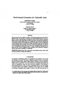
Defeaters, denoted by A ∼> p, do not actively support conclusions, but can only prevent some of them. If Alice, for example, would like to express the fact that she may not like cover versions of rock songs, she would have to formalize the defeater: r2’: cover(X) ∼> ¬likes(X). This defeater can defeat, for example, rule r2 mentioned above and it can be represented by Fig. 3. Rule r2’ actually introduces ambiguity regarding cover songs and Alice’s preferences, which should be resolved through other rules. However, the defeater alone cannot actively support the conclusion that Alice does not like a song, simply because it is a cover version.

cover(X)

likes(X) r2’

¬

¬

Fig. 3. Visual representation of defeater r2′.

Finally, the superiority relationship among the rule set R is an acyclic relation > on R, used, in order to resolve conflicts among rules. For example, given the defeasible rules r2 and r3 above, no conclusive decision can be made about whether Alice does like hard rock music or not, because rules r2 and r3 contradict each other. But if the superiority relationship r3 > r2 is introduced, then r3 overrides r2 and we can indeed conclude that Alice does not like hard rock. In this case, rule r3 is called superior to r2 and r2 inferior to r3. A fourth connection type is introduced for superiority relationships, which is displayed in Fig. 4. r3

>>>>>>>>>>>>>>>

r2

Fig. 4. Visual representation of r3 > r2.

According to defeasible logic proof theory,10 in order to show that q is provable defeasibly there are two choices: (1) to show that q is already definitely provable, using a strict rule; or (2) to show that there is a strict or defeasible rule with head q whose body

Visual Modeling of Defeasible Logic Rules with DR-VisMo 907

literals have been defeasibly proven and there are no possible “attacks”, that is, reasoning chains in support of ¬q. Formally, we must show that ¬q is not definitely provable. Also we must consider the set of all rules which are not known to be inapplicable and which have head ¬q (here we consider defeaters, too, whereas they could not be used to support the conclusion q). Essentially each such rule attacks the conclusion q. For q to be provable, each attacker must be counterattacked by another rule with head q with the following properties: (i) the counter-attacker must be applicable, and (ii) it must be stronger than (i.e. superior to) the attacker. Thus each attack on the conclusion q must be counterattacked by a stronger rule. 2.2. Representing arguments and conditions So far we have shown how rules are represented by interconnecting literal boxes with rule nodes. However, we have not yet included how literal arguments are presented, either being variables or constants. Also, variables are usually associated with simple conditions, such as Y>=1960, which could be represented as predicates, but it is practically more convenient to consider them more closely related to the closest literal that contains the corresponding variable as an argument. Arguments are incorporated inside the literal box just after the predicate name. The set of all arguments for each literal box is called argument pattern. For instance, the literal year(X,2000), which could state that the year a song X was released is 2000, is represented as in Fig. 5 (a). Simple conditions associated with any of the variables of a literal can also appear inside the literal box, each on a separate line (called condition pattern) below the literal. For example, if the fragment year(X,Y),Y>=1960 appears in a rule condition, it can be represented as in Fig. 5 (b). A certain predicate, say year, can appear many times in a rule base, in rule conditions or even rule conclusions. All literal boxes of the same predicate can be grouped, so that the user can realise that all these boxes refer to the same set of literals. To this end, we introduce the notion of a predicate box, a container for all literal boxes that refer to the same predicate. The literal boxes inside the predicate box "share" the predicate name that is located at the top of the predicate box. This approach is a temporary convention, needed in order to introduce the complete representation in the following sections. The literal boxes inside predicate boxes that express conditions on instances of the specific predicate extension are called predicate patterns. For example, the literal boxes of Fig. 5 can be grouped inside a predicate box as in Fig. 6. Notice that each predicate pattern contains exactly one argument pattern and zero, one or more condition patterns.

(a)

year(X,2000) ¬

(b)

year(X,Y) Y >= 1960 ¬

Fig. 5. Representing (a) arguments of literals and (b) simple conditions on variables.

908 E. Kontopoulos et al.

year (X,2000) ¬ (X,Y) Y >= 1960 ¬

Fig. 6. Predicate box and predicate patterns.

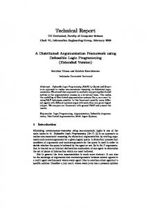
3. DR-VisMo: Defeasible Reasoning — Visualizing and Modeling DR-VisMo is a visual rule editor that assists users in modeling and visualizing defeasible logic rule bases. It is implemented as part of the VDR-DEVICE 8 system, an integrated development environment for deploying defeasible logic rule bases on top of RDF ontologies. The core component of VDR-DEVICE is DR-DEVICE,11 a reasoning system that processes RDF data, performs the defeasible inference procedure, produces the results and exports them as RDF data. The reasoning system employs an object-oriented RDF data model, which is different from the established triple-based RDF data model, treating properties as typical encapsulated attributes of resource objects. This way, properties of resources are not scattered across several triples, as in most other RDF inference systems, increasing query performance due to fewer joins.12 DR-DEVICE rule bases are expressed in an extension11 of RuleML. Extensions deal with two aspects of DR-DEVICE, namely defeasible logic and its CLIPS13 implementation. Defeasible logic extensions include rule types, superiority relations and conflicting literals, while CLIPS-related extensions deal with constraints on predicate arguments and functions. A fragment of a rule is displayed in Fig. 7. The names (rel elements) of the operator (_opr) elements of atoms are class names, since atoms actually represent CLIPS objects.13 RDF class names, used as base classes in the rule condition, are referred to via the href attribute of the rel element (e.g. hard_rock in Fig. 7, which responds to hard rock songs), while derived class names are text values of the rel element. Atoms have named arguments (slots), which correspond to object/RDF properties. Since RDF resources are represented as CLIPS objects, atoms in the rule body correspond to queries over RDF resources of a certain class with certain property values, while atoms in the rule head correspond to templates of materialized derived objects, which are exported as RDF resources at the end of the inference process.11,12 The following two sections describe the processes of developing (section 3.1) and visualizing (section 3.2) a defeasible logic rule base with the help of DR-VisMo, while section 3.3 presents the system architecture and functionality.

Visual Modeling of Defeasible Logic Rules with DR-VisMo 909

3.1. Rule base development The rule base graph consists of a variety of elements. Initially, for each class that the user wants to be created, a class box with the same name is constructed. Class boxes are the equivalent of predicate boxes, described previously, and they are populated with one or more class patterns, the equivalent of predicate patterns. In practice, class patterns express selection conditions over instances of the specific class. Visually, class patterns appear as literal boxes. This mapping is justified by the fact that atoms – expressed in the RuleML-like language of VDR-DEVICE – are actually atomic formulas (they correspond to queries over RDF resources of a certain class with certain property values). Thus, the truth value associated with each returned class instance will be either positive or negative. Similarly to class boxes, class patterns are populated with one or more slot patterns, which are the equivalent of argument and condition patterns. There are, however, certain differences that arise from the different nature of the tuple-based model of predicate logic and the object-based model of VDR-DEVICE. In the latter, class instances are queried via named slots rather than positional arguments. Not every slot needs to be queried and the position of the slot inside the object is irrelevant. Therefore, instead of a single-line argument pattern there is a set of slot patterns in many lines; each slot pattern is identified by the slot name. Furthermore, in the VDR-DEVICE RuleML-like syntax, simple conditions are attached to the slot patterns; this is reflected to the visual representation where condition patterns are encapsulated inside the associated slot patterns. An example of all the above is seen in Fig. 7, which shows a class box (created with DR-VisMo) that contains three class patterns applied on the hard_rock class and a code fragment matching the third class pattern, written in the RuleML-like syntax of VDRDEVICE. The class patterns contain 1, 2 and 3 slot patterns respectively. The argument list of each slot pattern is divided in two parts, separated by a colon; the variable is placed on the left and the corresponding expressions and conditions are placed on the right. The x "Rainbow" y y 1980

Fig. 7. A class box example and a code fragment for the second class pattern.

910 E. Kontopoulos et al.

variable in the slot pattern is used, in order for the slot value to be unified, with the latter having to satisfy the list of constraints. In other words, slot patterns represent conditions on slots (or class properties). In the case of constant values, only the left-hand side is utilized; the second and third class patterns, for instance, contain such examples. To sum things up, the first class pattern represents a query on all instances of the hard_rock class that have a name, i.e. all the named hard-rock songs; the second class pattern queries all the named hard-rock songs that were performed “live”, while the third one represents a query on all the hard-rock songs by the “Rainbow” band that were released after 1980. Besides class boxes, class patterns and slot patterns, users can also create rule circles that represent rules and arcs that connect the nodes in the graph. Rule circles contain the unique rule ID assigned by the user and their appearance was described in a previous section. As for the connections in the graph, there exist five types of them, as stated earlier: three for the rule type (strict, defeasible, defeater), one for the superiority relationship, plus a simple arrow connection type for connecting the class patterns of rule bodies to the rule circles. A sample rule graph, containing several of the features described above can be seen in Fig. 9. 3.2. Rule base visualization Besides modeling defeasible logic rule bases, DR-VisMo can also visualize an existing rule base. The first step involves collecting the class names. 3.2.1. Collecting the class names The RDF Schema documents, designated by the user, are being parsed and the names of the classes found are collected in the base class set (CSb), which already contains rdfs:Resource, the superclass of all RDF user classes: CSb := { rdfs:Resource } foreach 〈 S, P, O 〉 ∈ RDFS if P=rdf:type and O=rdfs:Class then CSb := CSb ∪ { S } where RDFS represents the set of all subject-predicate-object triples found in the RDF Schema documents. There also exists the derived class set (CSd), containing the names of the derived classes, i.e. classes which lie at rule heads (conclusions). CSd is initially empty and is dynamically extended every time a new class name appears inside the rel element of the atom in a rule head (or a negated atom). CSd := ∅ foreach c ∈ rel(_opr(atom(_head(imp)))) ∪ rel(_opr(atom(neg(_head(imp)))))

CSd := CSd ∪ { c } The function f1(f2(…fn(x))) evaluates the XPath expression //x/fn/…/f2/f1 and returns the corresponding node-set. When there is a single clause f, it simply corresponds to the expression //f. Attributes are retrieved via the composite function @f, which

Visual Modeling of Defeasible Logic Rules with DR-VisMo 911

corresponds to the expression //@f. CSd is mainly used for loosely suggesting possible values for the rel elements in the rule head, but not constraining them, since rule heads can either introduce new derived classes or refer to already existing ones. Notice that in some rules the atom element may not be the direct child of the _head element because a neg element may lie in between. The union of the above two sets results in the full class set CSf (CSf := CSb ∪ CSd), which is used for constraining the allowed class names, when editing the contents of the rel element inside atom elements of the rule body. 3.2.2. Determining class boxes, class patterns and slot patterns Class Boxes, Class Patterns and Slot Patterns are objects needed to visualize the classrelated nodes of the rule graph. The structure of these objects is depicted in Table 1. Table 1. The structure of class boxes, class patterns and slot patterns.

Class name

Attributes

Explanation

Class Box (C_B)

N P N Body Head S In

Class box name The set of class patterns of a class box Name of corresponding class box The rule in the body of which the class pattern appears The rule in the head of which the class pattern appears The set of slot patterns of a class pattern The rule arrow that ends in the class pattern (when the class pattern is a conclusion of a rule) The class arrow that emanates from the class pattern (when the class pattern is in a rule body) Slot pattern name The list of variables of a slot pattern The list of constraints of a slot pattern

Class Pattern (C_P)

Out Slot Pattern (S_P)

N Var Constraint

For each class c, a class box cb with the same name is constructed and placed inside the corresponding class box set CBb, CBd and CBf : CBb := ∅

CBd := ∅

foreach c ∈ CSb create cb of class C_B

foreach c ∈ CSd create cb of class C_B

CBb := CBb ∪ { cb } cb.N := c

CBd := CBd ∪ { cb } cb.N := c CBf := CBb ∪ CBd

Class boxes are initially empty and are dynamically populated with one or more class patterns as follows: for each atom element a inside a rule head or body, a new class pattern cp is created and is inserted into the class box, whose name cb matches the class name that appears inside the specific atom. The set of all class patterns is denoted by CP.

912 E. Kontopoulos et al.

CP := ∅ foreach r ∈ imp foreach a ∈ atom(_body(r)) ∪ atom(neg(_body(r)) foreach cb ∈ CBf

cb.P:= ∅ if cb.N = rel(_opr(a)) then create cp of class C_P

cb.P := cb.P ∪ { cp } cp.N := cb.N cp.Body := @ruleID(_rlab(r)) CP := CP ∪ { cp } There is a corresponding procedure for the class patterns of the rule heads: foreach r ∈ imp foreach a ∈ atom(_head(r)) ∪ atom(neg(_head(r)) foreach cb ∈ CBf

cb.P:= ∅ if cb.N = rel(_opr(a)) then create cp of class C_P

cb.P := cb.P ∪ { cp } cp.N := cb.N cp.Head := @ruleID(_rlab(r)) CP := CP ∪ { cp } Similarly to class boxes, class patterns are empty, when they are initially created, but are soon populated with one or more slot patterns. For each _slot element inside an atom, a slot pattern sp is created that consists of a slot name (contained inside the corresponding attribute) and, optionally, a variable and a list of value constraints. Slot pattern sp is then inserted into the storage of the class pattern cp that corresponds to the relevant atom a. The set of all slot patterns is denoted by SP. SP := ∅ foreach α ∈ atom foreach s ∈ @name(_slot(a)) foreach cb ∈ CBf foreach cp ∈ cb.P if cb.N = rel(_opr(a))) then create sp of class S_P

SP := SP ∪ { sp } sp.N := s cp.S := cp.S ∪ { sp }

Visual Modeling of Defeasible Logic Rules with DR-VisMo 913

Each of the slot pattern parts (slot name, variable and list of value constraints) is being retrieved from the children (direct and indirect) of the _slot element in the XML tree representation of the rule base. foreach α ∈ atom foreach s ∈ _slot(a) foreach v ∈ var(s) ∪ var(_and(s)) foreach cb ∈ CBf foreach cp ∈ cb.S foreach sp ∈ cp.S if cb.N=rel(_opr(a)) ∧ sp.N=@name(s) then sp.Var:= sp.Var ∪ { v } foreach c ∈ ind(s) ∪ _not(s) ∪ ind(_and(s)) ∪ function_call(_and(s))) foreach cb ∈ CBf foreach cp ∈ cb.S foreach sp ∈ cp.S if cb=rel(_opr(a)) ∧ sp.N=@name(s) then sp.Constraint:= sp.Constraint ∪ { c }

3.2.3. Rule circles and arrow types Rule Circles and Arrows are objects that are needed in order to visualize the rule nodes and the arcs of the rule graph. The structure of these objects is depicted in Table 2. Note that some of the attributes above are applied later on, in section 3.2.4, where the algorithm for visualizing a rule base is thoroughly presented. Table 2. The structure of rule circles and arrows.

Class name

Attributes

Explanation

Rule Circle (R_C)

N In Out N In Out Type Orient SUP INF In Out In Out N

Rule name The set of incoming arrows The outgoing arrow Rule name The rule circle from which the arrow emanates The class box node to which the arrow ends The arrow type (plain|expandable – see section 3.2.4) The arrow orientation (plain|dotted – see section 3.2.4) The superior rule of the superiority relation The inferior rule of the superiority relation The rule circle from which the arrow emanates The rule circle to which the arrow ends The class pattern node from which the arrow emanates The rule circle to which the arrow ends A tuple of the class pattern and the corresponding rule that uniquely identifies the class arrow

Rule Arrow (R_A)

Superiority Arrow (SR_A)

Class Arrow (C_A)

914 E. Kontopoulos et al.

For every rule in the rule base a rule circle is constructed, whose name matches the value of the ruleID attribute in the _rlab element of the corresponding rule. The set of all rule circles is denoted by RC and all rules are included in the rule set RS. The rule type is equal to the value of the ruletype attribute inside the _rlab element of the respective rule and can only take three distinct values (strictrule, defeasiblerule, defeater). The corresponding arrow sets are denoted by SA, DA and FA. The set of all arrows originating from rule circles is denoted by RA. Rule circles are connected with the arrows representing rules, regardless their type. RS := RC := SA := DA := FA := ∅ foreach r ∈ imp

RS := RS ∪ { r } create rc of class R_C create ar of class A_R rc.N := ar.N := @ruleID(_rlab(r)) RC := RC ∪ { rc } rc.Out := ar ar.In := rc if @ruletype(_rlab(r)) = strictrule then

SA := SA ∪ { ar } rc.Type := strictrule if @ruletype(_rlab(r)) = defeasiblerule then

DA := DA ∪ { ar } rc.Type := defeasiblerule if @ruletype(_rlab(r)) = defeater then

FA := FA ∪ { ar } rc.Type := defeater RA = SA ∪ DA ∪ FA The superiority relationship is represented as an attribute (superior) inside the superior rule element. For each such relationship, a superiority arrow object is created, linking the superior rule with the inferior rule. The set of all superiority arrows is SRA. SRA := ∅ foreach r ∈ imp foreach sr ∈ @superior(_rlab(imp)) create sar of class SR_A

SRA := SRA ∪ { sar } sar.SUP := sar.In := @ruleID(_rlab(r)) sar.INF := sar.Out := sr r.Out := sr.In := sar

Visual Modeling of Defeasible Logic Rules with DR-VisMo 915

The arrows between the class patterns of the rule body and the rule circles are contained in the CA set: CA := ∅ foreach cp ∈ CP create car of class C_A

CA := CA ∪ { car } car.N := 〈 cp, cp.Body 〉 cp.Out := cp.Body.In := car car.In := cp car.Out := cp.Body car.Out.Premises := car.Out.Premises ∪ { cp } where the 〈cp, cp.Body〉 tuple uniquely identifies such arrows, because the same class pattern can be re-used in the body of many rules. What remains to be established is how the arrows between the rule circles and the class patterns of the rule head are constructed. These arrows are contained in the RA set, presented above. Class patterns of the rule head are connected to rule arrows as follows: foreach ar ∈ RA foreach cp ∈ CP if cp.Head = ar.N then

cp.In := ar ar.Out := cp ar.In.Conclusion := cp 3.2.4. The visualization algorithm After having collected all the necessary graph elements and having populated all the class boxes with the appropriate class and slot patterns, three sets exist: (i) the base class boxes set CBb that contains the class boxes corresponding to base classes, (ii) the derived class boxes set CBd that contains the class boxes corresponding to derived classes, and (iii) the set RC that includes all the rule circles of the rule base. The next important task is the placement of each element in the graph. To this end, an algorithm for the visualization of the rule base was implemented, which utilizes common rule stratification techniques.14 Unlike the latter, however, that focus on computing the minimal model of a rule set, our algorithm aims at the optimal visualization outcome, namely the simplest graph possible. The algorithm is displayed in Fig. 8. The algorithm gives a left-to-right orientation to the flow of information, placing the graph elements in strata (or columns), with the first stratum located on the utmost left and the numbering of the strata following the same left-to-right orientation. In other words, the proposed algorithm deals with the “stratification” of the graph elements, calculating the optimal stratum, in which each graph element has to be placed.

916 E. Kontopoulos et al.

During the execution of the algorithm, the following steps can be distinguished: (i) All the base class boxes are placed in stratum #1. (ii) The algorithm enters a loop, consecutively assigning strata to rule circles and derived class boxes, incrementing each time the stratum counter by 1. (a) A rule circle is assigned to a stratum, when all its premises belong to previous strata, with at least one of them belonging to the immediately previous stratum. (b) A class box is assigned to a stratum, if it contains the conclusions of rules in the immediately previous stratum. str:=1 foreach cb∈CBb do cb.Stratum:=str while |RC|≠0 do RuleTemp:=∅ str:=str+1 foreach R∈RC do if ((∀p∈R.Premises → p.N.Stratum