VISUALIZATION BY EXAMPLE A CONSTRUCTIVE VISUAL COMPONENT-BASED INTERFACE FOR DIRECT VOLUME RENDERING Bingchen Liu and Burkhard W¨unsche and Timo Ropinski University of Auckland, Private Bag 92019, Auckland, New Zealand University of M¨unster, M¨unster, Germany
[email protected],
[email protected],
[email protected]
Keywords:
Direct volume rendering, transfer functions, visual interfaces, visualizations, histograms
Abstract:
The effectiveness of direct volume rendered images depends on finding transfer functions which emphasize structures in the underlying data. In order to support this process, we present a spreadsheet-like constructive visual component-based interface, which also allows novice users to efficiently find meaningful transfer functions. The interface uses a programming-by-example style approach and exploits the domain knowledge of the user without requiring visualization knowledge. Therefore, our application automatically analysis histograms with the Douglas-Peucker algorithm in order to identify potential structures in the data set. Sample visualizations of the resulting structures are presented to the user who can refine and combine them to more complex visualizations. Preliminary tests confirm that the interface is easy to use, and enables non-expert users to identify structures which they could not reveal with traditional transfer function editors.
1
Introduction
Direct Volume Rendering (DVR) is a popular technique for exploring and visualizing 3D data sets directly without requiring intermediate representations. Traditional DVR is described by the emissionabsorption model, where scalar values are interpreted as densities of a gaseous material which emits and absorbs light. An image is created by accumulating the total light intensity for each pixel of a view plane. This computation requires the definition of transfer functions which associate intensities in the volume with optical properties, i.e., color and opacity. The main challenge in DVR is to find transfer functions which reveal structure in the data, differentiate materials and reveal relationships between different structures. This requires an appropriate choice of colors, opacities and boundaries between different materials which requires careful selection of the shape, extend and value of the color and opacity transfer functions. This task is especially challenging for users without visualization experience. Our preliminary tests with four inexperienced users revealed that none of them was able to create meaningful visualizations for medical imaging data sets without a detailed
explanation of a traditional transfer function design interface. Furthermore, the users required a detailed explanation of what to look for and how these structures are represented in the data set’s histogram. In order to make DVR available to a wider range of users a more intuitive and easy-to-use interface for exploring data sets must be found. In this paper we present a novel spreadsheet-style interface which allows inexperienced users to utilize DVR applications without having to study the complex underlying mathematical and optical models. Section 2 reviews existing interfaces for transfer function design. Sections 3 and 4 present the design and implementation details of our interface. Visualization results and the findings of a preliminary user study with our new interface are discussed in Section 5. Section 6 concludes the paper and discusses future work.
2
Literature Review
Existing tools for transfer function design can be differentiated into image- and data-driven algorithms and combinations of them (Yoo et al., 2002). Initial
research in transfer function design utilized a datadriven approach, i.e., the transfer functions resulted from an analysis of the underlying data set. Kindlmann and Durkin use the data values, first derivatives and second derivatives to construct a 3D histogram in which they detect boundary features (Kindlmann and Durkin, 1998). Sato et al. improve material differentiation by characterizing local structures into linelike, sheet-like, and blob-like features (Sato et al., 2000). Kindlmann et al. present curvature-based transfer functions using a convolution-based derivative measurement scheme (Kindlmann et al., 2003). Caban et al. search for texture patterns in the data set in order to differentiate materials (Caban and Rheingans, 2008). Due to the lack of intuitive relationship with the resulting visualization, data-driven methods can be considered as less suitable for interactive approaches – especially for inexperienced users. In contrast image-driven transfer function design methods enable users to interact directly with the visualization. An early example (He et al., 1996) uses randomly generated or predefined transfer functions. The resulting DVR images are presented to the user as a table and are iteratively used to create new transfer functions. Jankun-Kelly and Ma (Jankun-Kelly and Ma, 2001) use a spreadsheet-like interface, which captures all parameters modifications and intermediate visualization results. This allows the user to modify parameters of the transfer functions and DVR algorithm based on desirable previous visualization results. In order to get more control about the visualization results a higher-dimensional transfer function can be used. Tzeng et al. have chosen this way and provide a sketch interface which enables users to indicate regions of high and low interest in image slices (Tzeng et al., 2003). A similar but more direct approach is used by Ropinski et al. (Ropinski et al., 2008). The user selects a feature of interest by drawing strokes directly onto the volume rendering near its silhouette. The information is used to identify the feature in the histogram space and generate an appropriate component transfer function. A promising approach is to combine the advantages of both data- and image-driven approaches. Kniss et al. achieve this by allowing the user to place data probes into the visualization to capture regions of interest (Kniss et al., 2002). The underlying data is then highlighted in a multi-dimensional histogram (e.g., data values and first derivatives) and multidimensional transfer functions can be constructed using interactive widgets in order to capture these features. While the interface is intuitive and flexible the last step requires some knowledge of visualizations and DVR.
3
Design
The goal of our research is to create a DVR interface for users without any experience in visualization and DVR. Our only assumption is that the user has some knowledge of the application domain. Since the human brain has highly evolved pattern recognition and 3D perception abilities we propose a visual “programming-by-example” approach: the user is presented basic visualizations of the data set and has to assemble more complex ones by interacting with the images. This requires solutions to the following three problems. Automatically create basic visualizations which provide a good basis for exploring the data set and creating complex meaningful visualizations. Present the visualizations in a way which enables the user to assess and select desirable visualizations. Provide an interface which allows the user to combine, refine and modify existing visualizations.
3.1 Unit Transfer Functions As seen in Section 2, designing a complex meaningful transfer function is difficult. A possible solution to that problem is to create simple visualizations which the user recognizes or at least can comprehend and to “assemble” them to more complex ones using the user’s application domain knowledge. To generate such simple visualizations we introduce “unit transfer functions”, which visualize only one structure in the data set. In order to provide a good basis for exploration, the unit transfer function must cover a wide variety of structures (different material properties). Previous research has demonstrated that structures in a scalar volume data set can often be characterized by the first and second order derivatives (Kindlmann and Durkin, 1998). A region is classified as boundary material, when two materials are relatively thick and have a thin transition region or if two materials have very different densities in which case the densities increase/decrease rapidly throughout the transition region. In either case the materials form a peak and the transition region a valley in the resulting histogram. We can therefore characterize many structures as peaks in the histogram where the size (number of voxels) of a peak corresponds to the size of the corresponding structure(s). We can hence construct unit transfer function as follows: We generate a histogram by creating a bin for each value of the range of density values in the data set and compute the number of voxels with that value. Since the difference between maximum and minimum values of bins often varies dramatically we use the normalized logarithmic values of
the original histogram values (we use the function log(ValueO f T heCurrentBin)/log(MaxValue)). The histogram is represented by a 2D curve where each tuple (binValue, #voxelsWithThatValue) is a point. The key element of our algorithm is to simplify this curve and identify its main peaks (key features of the original histogram). We achieve this by using the Douglas-Peucker algorithm (Peucker, 1973), which works as follows. Specify an ε value for the maximum allowed error of the approximated curve. In our case this value corresponds to the size of features we capture. For ε = 0 we get the original smoothed histogram and for ε = maximumBinValue we get only one peak corresponding to the peak of the histogram. Afterwards a polyline S is created, which initially only contains the first and last point of the curve (left and right most value in the histogram). Then the distances of all points to the line are computed. If the maximum distance is smaller than ε then stop. Otherwise add the point P which is of maximum distance to the line to S and call the algorithm recursively for the two sections of the curve on either side of P. Figure 1 demonstrates the effect of applying this algorithm.
3.2 Spreadsheet-Like Interface In order to achieve a “programming-by-example” approach, we use two spreadsheet-like tables to display the current and previous visualization results. The first row contains initially the automatically generated unit transfer functions. The user can select meaningful images and add them to the second row containing previous visualizations. One or multiple visualizations in of this section can then be selected and modified, combined or refined – the results are displayed in the top row. The bottom section of the interface contains the buttons for the operations for modifying visualizations (by modifying the underlying transfer functions). Figure 2 demonstrates the interface. The histogram in the bottom-left is for illustrative and testing purposes and is not shown to inexperienced users.
Figure 2: The spreadsheet-like interface defining complex transfer functions. Figure 1: The red line represents the original histogram of the nucleon data set in Figure 4 and the black line represents the result of applying the Douglas-Peucker algorithm with ε = 10 to the histogram. Note that the second curve is scaled in y-direction to improve readability.
3.3 Operations on Unit Transfer Functions
We sort the peaks in the resulting histogram by importance (currently determined by their height relative to the valleys on either side) and define for each peak a unit transfer function capturing only the region represented by that section of the histogram. Each unit transfer function is associated with one random color value and an opacity value which increases linearly with the density value of the corresponding peak in the histogram. Note that this decision makes the assumption that the region with the highest density are inside the data set and regions with lower density outside. This is the case for many physical and medical data sets, e.g., computed tomography (CT) where the density of bone is higher than the density of muscle which in turn is higher than that of fat and skin.
The user can “assemble” complex transfer functions out of the selected unit transfer functions by using the following operations: The “search around a feature” function is applied to one visualization selected by the user. It finds the peaks in the histogram surrounding the peak corresponding to the transfer function of the current visualization and creates unit transfer functions for them. Note that in contrast to the initial selection of peaks this approach selects any peak regardless of the size and the height of the peak. The “interpolation” function is applied to two visualizations selected by the user. It examines the section of the histogram between the peaks of the corresponding transfer functions and then finds the three largest peaks within it or, if there are no peaks, places
the transfer functions equidistantly in between. This is achieved by using the Douglas-Peuker algorithm with decreasing ε values until three peaks are found or until ε = 2. The “merge” function combines selected visualizations. Currently it can only be applied to unit transfer functions and is achieved by combining them and removing any overlapping sections as indicated in Figure 3.
Figure 3: Merging of two overlapping transfer functions (left) and the results after removing the overlapping section (right).
4
Implementation
less than 30 seconds and was achieved by simply combining the visualizations corresponding to the automatically created unit transfer functions. In contrast, an experienced user required about 90 seconds for generating a comparable transfer function with the original Voreen interface. Besides the used colors, which are so far randomly assigned in our approach, the results where almost identical. The example shown in Figure 4, is a simulation of the two-body distribution probability of a nucleon in the atomic nucleus (8Bit, 41 3 voxels) obtained from www.volvis.org. We asked an inexperienced student to create a meaningful visualization with both the traditional transfer function design interface within Voreen (Meyer-Spradow et al., 2009) and our interface. The first row of Figure 4 shows the visualization rendered with Voreen, where the transfer functions has been manually defined by the user. The second row shows the visualization obtained with our interface. The third row shows the unit functions used to generate the visualization in row one. The fourth row shows the transfer function generating the visualizations in row two. This transfer function has been generated with Voreen’s standard transfer function editor.
Our implementation is based on Voreen (MeyerSpradow et al., 2009), a rapid-prototyping environment for ray-casting-based volume visualizations. Voreen uses GPU-acceleration for rendering, which is abstracted through an object-oriented structure, which represents each phase of the DVR process as individual processors. Since Voreen is developed with C++ and the Qt UI framework, we develop our interface with Qt and integrate Voreen using a QWidget. We set up all rendering steps of the DVR process by defining a standard DVR network. Each transfer function is stored as a TransFuncIntensity object and associated with a VoreenPainter object and connected with a QtCanvas representing a cell in the spreadsheet.
5
Results
We have evaluated our tool by using real and simulated data sets from different application fields.
5.1 Visualization Results For the NCAT phantom dataset (8 Bit, 128 3 voxels) shown in Figure 2, we asked a computer science student without any experience in medical imaging to generate a transfer function with our technique. Creating the visualization took this inexperienced user
Figure 4: Nucleon dataset DVR visualization. It includes the visualization generated directly with Voreen in the first row, the visualization generated with our interface in the second row, the unit function used in our interface in the third row, and the transfer function used in the visualization of Voreen in the last row.
It can be seen that the manually defined transfer functions result in sharper “material boundaries” and more appropriate opacity values which makes shape perception slightly easier. The reason for this is that our unit transfer functions always have a triangle shape and the user can not modify opacity values. Note that the two visualizations seem to show different “material boundaries”. Both solutions
are correct, however, since the nucleus data set has smoothly varying values and hence the perceived material boundaries are purely illustrative. The surfaces give an indication of the density value change, but they do not indicate different “materials”. Overall, the user in our test found it considerable easier to create the visualization with our interface and required much less time. Figures 5 and 6 show two further examples using real world data sets. Note that in both examples our interface results in meaningful visualizations. Our method has limitations, though, as is illustrated by the expert visualizations in figure 7. It can be clearly seen that the visualization of the two feet CT using the traditional Voreen interface shows considerable more structures. The main reasons for this are that some tissue structures do not correspond to histogram peaks, but also that tissue boundaries have been enhanced using shading functions.
Figure 6: Visualization of CT scan of two feet (16Bit, 256 × 256 × 250 voxels) provided by Osirix and visualized using our spreadsheet-like interface. The bottom left graph shows the original histogram (red) and its main peaks identified with the Douglas-Peucker algorithm (black).
Figure 5: Visualization of a Bonsai CT data set (8Bit, 2563 voxels) with our spreadsheet-like interface. The bottom left graph shows the original histogram (red) and its main peaks identified with the Douglas-Peucker algorithm (black).
5.2 Usability Our preliminary users tests suggest that meaningful visualizations can be constructed with our interface in less than a minute. Several users struggled with the nucleus data set in figure 4 because they did not know what it represents. None of the users was able to create high quality visualization of the CT feet data set because of the lack of relationship of data set features and histogram features. Users were also confused about the lack of spatial relationships when modifying visualizations. In particular they expected that refining a visualization would result in structures close to the currently visualized structure. This is often not the case since neighboring peaks in the his-
Figure 7: Expert results for the data sets in figure 5 and 6 obtained using the traditional Voreen transfer function interface.
togram can correspond to spatially completely unrelated structures.
5.3 Discussion Compared with a traditional transfer function design tool our approach is faster and required no knowledge of the DVR process and transfer functions. In
all cases we investigated our tool was able to create meaningful visualizations. Since the user does not have any direct control about the transfer functions the resulting visualizations can be less accurate than when using a traditional transfer function design tool. Our examples show that there are three implementation issues which must be resolved: The lack of color control can result in ambiguities if two different materials have very similar colors. The use of increasing opacity values for the peaks of the volume’s histogram works well for objects where the innermost structures have the highest densities, e.g., CT data sets, but is not a suitable solution for general applications. Finally the use of a one-dimensional histogram and the restrictions to identifying peaks in the histogram can be insufficient for identifying all structures in a data set.
6
Conclusion and Future Work
The usage of DVR in science, engineering and other application areas can be significantly expanded by providing users with a simple and intuitive tool for representing structure in the data. We have designed such a tool by combining a “programming-byexample” approach with an automatic transfer function design technique. In contrast to previous publication our transfer functions are defined as combination of so-called unit transfer function. Each unit transfer function captures one structure in the data set by representing one feature in the data set’s histogram. Features are identified by applying the Douglas-Peucker algorithm to the histogram curve. By choosing different epsilon values for the Douglas-Peucker algorithm features with different variations can be differentiated, which in many cases will correspond to an order by importance. Using a wide variety of data sets we have demonstrated, that complex visualization can be constructed without requiring knowledge regarding the DVR algorithm, transfer functions or image histograms. We have only just started to explore the possibilities offered with our new concept. Future research will concentrate on improved unit transfer functions as well as improved user interaction. Furthermore, we are interested in extending the technique to multidimensional transfer functions (Kniss et al., 2002). We also believe, that the usability of the tool can be improved by determining an optimal layout of the rendering results of unit transfer functions and intermediate visualization results, and by supporting the combination via drag-and-drop. Interaction with transfer
functions can be improved by adding sketch-based interfaces as presented in (Ropinski et al., 2008).
REFERENCES Caban, J. J. and Rheingans, P. (2008). Texture-based transfer functions for direct volume rendering. IEEE Transactions on Visualization and Computer Graphics, 14(6):1364–1371. He, T., Hong, L., Kaufman, A., and Pfister, H. (1996). Generation of transfer functions with stochastic search techniques. In VIS ’96: Proceedings of the 7th conference on Visualization ’96, pages 227–ff. Jankun-Kelly, T. J. and Ma, K.-L. (2001). Visualization exploration and encapsulation via a spreadsheet-like interface. IEEE Transactions on Visualization and Computer Graphics, 7(3):275–287. Kindlmann, G. and Durkin, J. W. (1998). Semi-automatic generation of transfer functions for direct volume rendering. In VVS ’98: Proceedings of the 1998 IEEE symposium on Volume visualization, pages 79–86. Kindlmann, G., Whitaker, R., Tasdizen, T., and Moller, T. (2003). Curvature-based transfer functions for direct volume rendering: Methods and applications. In VIS ’03: Proceedings of the 14th IEEE Visualization 2003 (VIS’03), page 67. Kniss, J., Kindlmann, G., and Hansen, C. (2002). Multidimensional transfer functions for interactive volume rendering. IEEE Transactions on Visualization and Computer Graphics, 8(3):270–285. Meyer-Spradow, J., Ropinski, T., Mensmann, J., and Hinrichs, K. (2009). Voreen: A rapid-prototyping environment for ray-casting-based volume visualizations. IEEE Computer Graphics and Applications, 29(6):6– 13. Peucker, D. D. . T. (1973). Algorithms for the reduction of the number of points required to represent a digitized line or its caricature. The Canadian Cartographer, 10(2):112–122. Ropinski, T., Praßni, J.-S., Steinicke, F., and Hinrichs, K. H. (2008). Stroke-based transfer function design. In IEEE/EG Volume and Point-Based Graphics, pages 41–48. Sato, Y., Westin, C.-F., Bhalerao, A., Nakajima, S., Shiraga, N., Tamura, S., and Kikinis, R. (2000). Tissue classification based on 3d local intensity structures for volume rendering. IEEE Transactions on Visualization and Computer Graphics, 6(2):160–180. Tzeng, F.-Y., Lum, E. B., and Ma, K.-L. (2003). A novel interface for higher-dimensional classification of volume data. In Proceedings of the 14th IEEE Visualization 2003 (VIS’03), page 66. Yoo, T., Gerig, G., Whitaker, R., Kindlmann, G., Machiraju, R., and M¨oller, T. (2002). Image processing for volume graphics. Course notes #50, ACM SIGGRAPH 2002.