Visually Augmented Navigation in an Unstructured Environment Using ...

Visually Augmented Navigation in an Unstructured Environment Using a Delayed State History Ryan Eustice∗ , Oscar Pizarro∗ and Hanumant Singh† ∗

MIT/WHOI Joint Program in Applied Ocean Science and Engineering Massachusetts Institute of Technology Cambridge, MA, USA † Department of Applied Ocean Physics and Engineering Woods Hole Oceanographic Institution Woods Hole, MA, USA {ryan, opizarro, hanu}@whoi.edu

Abstract— This paper describes a framework for sensor fusion of navigation data with camera-based 5 DOF relative pose measurements for 6 DOF vehicle motion in an unstructured 3D underwater environment. The fundamental goal of this work is to concurrently estimate online current vehicle position and its past trajectory. This goal is framed within the context of improving mobile robot navigation to support sub-sea science and exploration. Vehicle trajectory is represented by a history of poses in an augmented state Kalman filter. Camera spatial constraints from overlapping imagery provide partial observation of these poses and are used to enforce consistency and provide a mechanism for loop-closure. The multi-sensor camera+navigation framework is shown to have compelling advantages over a camera-only based approach by 1) improving the robustness of pairwise image registration, 2) setting the free gauge scale, and 3) allowing for a unconnected camera graph topology. Results are shown for a real world data set collected by an autonomous underwater vehicle in an unstructured undersea environment. Index Terms— navigation, sensor fusion, ego-motion, structure from motion, simultaneous localization and mapping, Kalman filtering

I. I NTRODUCTION Robotic exploration of remote environments extends our reach to areas where human exploration is considered too dangerous, too technically challenging, or both. The 2004 Mars exploration rover mission is one such example, another is deep ocean science. Deep ocean science has been an environment where humans have demonstrated that though they have the ability to build vehicles which can carry them to the deep, like the deep sea submersible Alvin [1], the human risk, operational cost, and limited availability prevent its wide spread use. Therefore, out of necessity deep ocean science and exploration has become an arena where the presence of mobile robotics is pervasive and their utility revolutionary [2]–[4]. The advent of the Global Positioning System (GPS) allows surface and air vehicles to know their position anywhere on the globe to within a few meters via triangulation of satellite transmitted radio signals. However, these radio signals do not penetrate sub-sea [5], underground [6], or even indoors. Therefore, typical methods for underwater navigation have focused on beacon-based navigation networks, such as long baseline

acoustic systems (LBL), which offer bounded error position measurements, but require the predeployment and calibration of the beacon network. In this navigation scheme, position updates are confined to an area of acoustic network coverage and require line-of-sight. Accuracies for low-frequency systems (12kHz) hover around meter level precision while higher frequency systems (300kHz) can obtain centimeter level performance at the expense of network range [5]. Another popular navigation strategy is to use inertial navigation systems (INS) and dead-reckoning (DR). These systems are accurate in the short-term, but exhibit an unbounded growth in error essentially as a function of time. With a DR navigation methodology, improved positional accuracy requires more precise, but increasingly expensive, INS sensors which in the end only slow down and do not stop the unbounded error growth. Within the past decade, the mobile robotics community has turned to environment based navigation methods which exploit perceptual sensing capabilities; a robot measures “features” in the environment and uses them to help localize. The question of how to use such a methodology for navigation and mapping began being theoretically addressed in a probabilistic framework in the mid 80’s with a seminal paper by Smith, Self, and Cheeseman [7]. The feature based navigation and mapping methodology has since been coined SLAM – simultaneous localization and mapping. The SLAM problem statement is deceptively simple, however much theoretical work has gone into how best to solve it. The problem is stated as: given uncertain vehicle pose measurements and uncertain measurements of features relative to the vehicle, concurrently estimate a map of features in the environment and the vehicle’s location within that map. Depending on the perceptual sensor of choice and characteristics of the typical operating environment, it may be difficult to define “features” to build a map with. In man-made structured environments, typically composed of planes, lines and sharp corners, features can be more easily defined [8]. Outdoor unstructured environments pose a more challenging task and many approaches have focused on techniques such a “scanmatching” [9] which do not require an explicit representation

of features, but do require an accurate perceptual sensor (e.g. a laser range finder) so that raw data can be matched directly (for example in an iterative closest point sense). Defining and acquiring features in the unstructured undersea realm is an even more challenging task since sharp corner, line, and plane primitives do not naturally exist and accurate perceptual range sensors like laser range finders have limited applicability. However, when navigating near the seafloor we can use a camera as an accurate and inexpensive perceptual sensor which can measure “features” in the environment. A camera encodes information about the scene, and indirectly, its pose relative to that scene. Point features in an unstructured environment naturally fit into a camera feature-based registration framework and allow for “zero-drift” measurements of pose referenced to the scene. When point features in the scene are not explicitly known (i.e. 3D structure is not recovered) pair-wise registration allows for “zero-drift” measurements of relative pose between camera frames. That is, registering an image taken from time ti to an image taken at time tj provides a measurement of relative pose whose error is bounded regardless of time or distance traveled between those instances. The rest of this paper presents our framework and methodology for incorporating camera based relative pose measurements with vehicle navigation data in a SLAM based context. Camera measurements are shown to enforce consistency and provide a mechanism for loop closing in a 3D unstructured undersea environment exercised over 6 DOF vehicle motion. We show that a multi-sensor approach has compelling advantages over a camera-only based navigation system. Results are presented in the context of a real-world data set collected by an autonomous underwater vehicle (AUV) in a rugged undersea environment. II. P LATFORM Our application is based upon using a pose instrumented AUV equipped with a single down-looking calibrated camera to perform underwater imaging and mapping [3]. The vehicle makes acoustic measurements of both velocity and altitude relative to the bottom. Absolute orientation is measured to within a few degrees over the entire survey area via inclinometers and a flux-gate magnetic compass. Bounded positional estimates of depth, Z, are provided by a pressure sensor. Table I characterizes the navigation sensor capabilities in our application. TABLE I

P OSE SENSOR CHARACTERISTICS . Measurement Roll/Pitch Heading 3-Axis Angular Rate Body Frame Velocities Depth Altitude

Sensor Tilt Sensor Flux Gate Compass AHRS Acoustic Doppler Pressure Sensor Acoustic Altimeter

Precision ±0.5◦ ±2.0◦ ±1.0◦ /s ±0.2cm/s ±0.01m ±0.1m

Power budget constraints force AUVs to use strobed lighting

for image acquisition. Energy consumption is proportional to the number of images taken. Therefore, in practice overlap is typically minimized so that survey range can be maximized [10]. III. T RAJECTORY E STIMATION In structure from motion (SFM) approaches, both camera motion and scene structure are recovered from a sequence of video frames. However, in our application the low degree of temporal image overlap (which is typically on the order of 25% or less) motivates us to instead focus on recovering pair-wise measurements of relative pose from image frames. Trajectory estimation is formulated within the context of SLAM, however in our implementation we do not keep an explicit representation of 3D features in the environment. Instead, a history of uncertain camera poses is maintained and defines our “map”. Pair-wise registration of images Ii and Ij therefore corresponds to a measurement of vehicle state at time tj relative to its previous state at time ti . Fleischer [11] proposed a similar undersea mosaic based navigation strategy for the problem of 2D translation-only navigation over a planar seafloor. His estimation framework combined 2D relative displacement measurements within the context of an augmented state Kalman filter (ASKF). Our work adopts his original idea of an ASKF for navigation and camera sensor fusion, but extends the incorporation of camera based relative pose measurements to a fully unstructured 3D undersea environment and 6 DOF vehicle motion. A. Augmented State Kalman Filter We begin by describing our representation of vehicle state and a general system model for state evolution and observation. This model is used as the basis for trajectory estimation within the context of an extended Kalman filter (EKF) [12]. We then show how to incorporate camera based relative pose measurements by augmenting our state representation to include a history of vehicle poses. The vehicle state vector and its associated covariance matrix are defined as: ¤ £ > > (1a) xv = x> p , xe · ¸ Pp Ppe Pv = (1b) Pep Pe Here xp is a six element vector of vehicle pose in the local-level reference frame where XYZ roll pitch heading Euler £ angles are used ¤> to represent orientation [13], i.e. xp = x, y, z, θ, φ, ψ . Any extraneous state elements required for propagation of the vehicle process model (such as velocities, accelerations, rates, etc) are represented by xe . The vehicle state evolves through a time-varying continuous time process model f v (·, t) driven by white noise w(t) v N (0, Q(t)), while discrete time measurements of elements in the vehicle state are observed through an observation model hv (·, tk ) corrupted by time independent Gaussian noise

£ v[tk ] v N (0, Rk ) where E wv> ] = 0.

x˙ v (t) = f v (xv (t), t) + w(t) z[tk ] = hv (xv [tk ], tk ) + v[tk ]

(2a) (2b)

¯ v and its covariance Pv are The estimated vehicle state x calculated using an extended Kalman filter whose equations are provided here for the system given in (2) [12]: Prediction x ¯˙ v (t) = f v (¯ xv (t), t) ˙Pv (t) = Fv Pv (t) + Pv (t)F> v + Q(t)

(3a) (3b)

Similarly, the navigation sensor observation model continues to remain only a function of the current vehicle state xv . However, camera based relative pose measurements between image frames Ii and Ij are a function of delayed states xpi and xpj and are discussed in III-C. B. Vehicle Process Model

Update ¤−1 £ − > > K = P− v H v H v Pv H v + R k ¤ £ ¯− ¯+ x− x v , tk ) v + K z[tk ] − hv (¯ v =x £ ¤ −£ ¤> P+ + KRk K> v = I − KHv Pv I − KHv

model for xaug continues to evolve the vehicle portion of the augmented state vector through the vehicle dynamic model f v while the delayed state entries are unaffected, i.e. ¸ · fv (xv (t), u(t), t) + w(t) (7) x˙ aug = 0[6N ×1]

(4a) (4b) (4c)

The EKF equations propagate linearized first order estimates of the via Jacobians ¯ mean and covariance ¯ ∂hv (xv [tk ],tk ) ¯ (xv (t),t) ¯ and H = . Fv = ∂f v∂x v (t) ∂x [t ] ¯ ¯ xv (t) xv [tk ] v v k Camera based relative pose measurements however, cannot be expressed with the fixed size state vector representation given in (1a). This is because registration of an image pair results in a relative pose estimate and not an absolute observation of elements in vehicle pose xp . We therefore must augment the state vector to include a history of delayed vehicle poses so that camera measurements can be incorporated. When the first image frame is captured at time t1 we augment our state vector with xp1 , i.e. the vehicle’s pose when it took image I1 . Therefore at time t1 the augmented state vector and covariance matrix are: ¸ · ¸ · xv [t1 ] xv [t1 ] ≡ (5a) xaug [t1 ] = xp [t1 ] xp [t1 ] · 1 ¸ · ¸ P [t ] Pvp [t1 ] Pv [t1 ] Pvp1 [t1 ] Paug [t1 ] = ≡ >v 1 Pvp [t1 ] Pp [t1 ] Pp1 v [t1 ] Pp1 [t1 ] (5b) This process is repeated for each camera frame which we wish to keep in our trajectory history. After augmenting N delayed states (one for each camera frame) and dropping the explicit time notation for conciseness we have: ¤ £ > > > (6a) xaug = x> v , x p1 , · · · , x pN   Pv Pvp1 · · · PvpN  Pp 1 v · · · P p1 pN  Pp 1   (6b) Paug =  . ..  . . . . .  . . .  . P pN Pp N v Pp N p 1 · · ·

Note that in (5b) the vehicle’s current pose xp is fully correlated with xp1 by definition. Therefore when the N th delayed state xpN is augmented in (6a) its cross-correlation with the other delayed poses in (6b) is non-zero since the current vehicle state has correlation with each delayed state. The system model given in (2) must be extended to incorporate the new augmented state representation. The process

In our particular application vehicle dynamics are typically low, therefore we choose to approximate the plant with a constant velocity process model. h i> ˙ φ, ˙ ψ˙ xe = u, v, w, θ, (8a) £ ¤> w = 0[1×6] , w1 , · · · , w6 (8b)    u R(θ, φ, ψ)  v     w     ˙  θ fv (xv (t), t) =  (8c)      φ˙      ψ˙ 0[6×1]

where u, v, w are body frame velocities, R(θ, φ, ψ) is an orthonormal rotation matrix from vehicle to local-level, and ˙ φ, ˙ ψ˙ are angular rates. The process model (8c) is both time θ, varying and nonlinear, therefore the EKF prediction update of (3) is solved between asynchronous navigation measurements using a 4th order Runge-Kutta approximation [14]. C. Camera Based Relative Pose Observation Model

Pairwise image registration has the ability to provide a measurement of relative pose between delayed state elements xpi and xpj , provided images Ii and Ij have overlap. The following camera observation model derivation uses homogeneous coordinate transformhnotationito derive the image based b b measurement where ba H = a0R t1ba denotes a transformation from frame a to frame b, ba R is an orthonormal rotation matrix from a to b, and b tba is a vector from b to a as expressed in frame b. The delayed state pose elements xpi and xpj encode the vehicle to local-level transformations `vi H and `vj H respectively. Therefore using the static camera to vehicle frame transform v c H, we can express the transformation from camera frame i to j as: cj ci H

c

= `j H

(9a)

=

(9b)

` ci H v −1` v −1` vi H c H cH vj H

c The resulting cji H can be decomposed into the 6 DOF relative c pose elements cji R and cj tcj ci which we denote simply as

R, t.

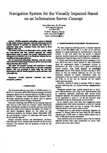
However, what the camera actually measures is a 5 not 6 DOF relative pose measurement. Loss of scale in the image formation process means that only the baseline direction t/ktk is recoverable from image space. Therefore, the camera based observation model between delayed states xpi and xpj is: £ ¤> zji = t> /ktk, θji , φji , ψji (10a) = hji (xaug ) (10b)   t/ktk   atan2(R1,3 sin(ψji ) − R2,3 cos(ψji ),    (10c) − R sin(ψ ) + R cos(ψ )) = ji ji 1,2 2,2   atan2(−R3,1 , R1,1 cos(ψji ) + R2,1 sin(ψji )) atan2(R2,1 , R1,1 ) IV. PAIRWISE I MAGE BASED R EGISTRATION Having incorporated camera-based relative pose measurements into our trajectory estimation framework, this section focuses on explaining how we actually make the image-based measurement. The core of our feature-based image registration engine is built around making pairwise measurements of relative pose. Pairwise wide-baseline registration is essential in our methodology for two main reasons: 1) Low overlap imagery is common in our temporal image sequences because of the nature of our underwater application domain. Typically images in the temporal sequence have 25% or less in common. 2) Loop-closing and cross-track spatial image constraints are the greatest strength of a camera based navigation system. It is these measurements which help to correct dead-reckoned drift and enforce recovery of a consistent trajectory. Wide-baseline viewpoints are typical in this scenario and would arise even if temporal overlap were much higher as with video-frame rates. Our feature-based registration algorithm loosely follows the “standard” computer vision approach presented in [15]. Fig. 1 illustrates the overall hierarchy of our feature-based algorithm which is built around: • Independently extracting features in each image using the Harris interest operator [16]. • Establishing an initial putative correspondence set based upon similarity and pose prior. • Robustly extracting an inlier correspondence set using a novel 6-point essential matrix algorithm [17] within the context of LMedS [18]. • Solving for an initial relative pose estimate based upon Horn’s algorithm [19] and regularized sampling from our relative orientation prior. • Refinement of the camera based relative pose estimate in a two-view bundle adjustment step [15]. The remainder of this section focuses on one of the more novel aspects of the above approach, namely using our relative pose prior to restrict correspondences.

A. Pose Restricted Correspondences The problem of initial feature correspondence establishment is arguably the most difficult and challenging task of a feature-

EKF Pose Prior Ri, ti

Ii

Ij

Feature Extract

Feature Extract

Feature Encode

Feature Encode

EKF Pose Prior Rj, tj

Pose Restricted Putative Correspondences

Robust Correspondences LMedS 6−pt Algorithm E Relative Pose Prior R, t

Horn’s Relative Pose Algroithm with Regularized Sampling of Orientation Prior

Two−View Bundle Adjustment

5 DOF Relative Pose Measurement & Covariance

Fig. 1. Overview of the pairwise relative pose estimation engine. Blue dashed lines represent additional information provided by prior pose. Given two images, we detect features using the Harris interest point detector. For each feature we then determine search regions in the other image by using prior pose and depth information. Putative matches are proposed based on similarity and constrained by the search regions. We then use LMedS and a 6-point essential matrix algorithm to establish a robust inlier correspondence set. Having established an initial correspondence set, an initial relative pose estimate is obtained via Horn’s algorithm with regularized sampling from our orientation prior. The initial pose estimate is then refined in a two-view bundle adjustment step by minimizing the reprojection error over all matches considered inliers.

based registration methodology. Having an initial estimate of prior pose can be used to great advantage in solving for correspondences and is something which is naturally available in the instrumented ASKF framework. Given uncertain prior motion knowledge, robustness to incorrect matches can be achieved by restricting the correspondence search to localized regions. Prior pose knowledge relaxes the demands on the complexity of the feature descriptor since the descriptor is no longer required to be unique globally, but only locally. We use the epipolar geometry constraint expressed as a two-view point transfer model to restrict the correspondence search. Pose uncertainty is propagated through the model to derive first-order estimates of the bounded search regions. This region is used to restrict the interest point matching to a set of candidate correspondences relaxing the demands of and improving the robustness of the feature based similarity matching. 1) Point Transfer Mapping: Zhang first characterized epipolar geometry uncertainty in terms of the covariance matrix of the fundamental matrix [20]. In [21] prior pose knowledge is used to constrain the search space by propagating pose uncertainty to the epipolar line. However, both of these characterizations of uncertainty are hard to interpret in terms of physical parameters. The following presents a point transfer mapping which benefits from a more physical interpretation,

and an increased robustness by making use of scene range data if available. Our pose constrained search methodology is similar to [22], however, they assumed a CAD model of the environment existed. In this derivation of the point transfer mapping we assume projective camera matrices P = K[I | 0] and P0 = K[R | t], where K is the matrix of intrinsic camera parameters [15], and R, t are the relative orientation parameters. Given an interest point with pixel coordinates (u, v) in > image I, we define its vector representation u = [u, v] , as well as its normalized homogeneous representation u = [u> , 1]> . Likewise we define the imaged scene point as X = [X, Y, Z]> and its normalized homogeneous representation X = [X> , 1]> . We note that equality in expressions involving homogeneous vectors is implicitly defined up to scale. The scene point X is projected through camera P as u = PX = KX

(11)

which implies that including scale we have X ≡ ZK−1 u

(12)

This back-projected scene point can subsequently be reprojected into image I 0 as u0 = P0 X = K(RX + t)

(13)

By substituting (12) into (13) and recognizing that the following relation is up to scale, we obtain the homogeneous point transfer mapping [15] u0 = KRK−1 u + Kt/Z

(14)

Finally, by explicitly normalizing the previous expression and defining H∞ = KRK−1 [15], we recover the nonhomogeneous point transfer mapping u0 =

H∞ u + Kt/Z H3T ∞ u + tz /Z

(15)

where H3T ∞ refers to the third row of H∞ , and tz is the third element of t . When the depth of the scene point Z is known in camera frame c, then (15) describes the exact two-view point transfer mapping. However, when Z is unknown (15) describes a functional relationship on Z (i.e. u0 = f (Z)) which traces out the corresponding epipolar line in I 0 . 2) Point Transfer Mapping with Uncertainty: The delayed vehicle poses in our ASKF representation are uncertain and are defined with respect to the local-level reference frame. Therefore the relative pose measurement required in (15) must be composed by going through this intermediate frame as shown in (9). A first-order estimate of the uncertainty associated with the point transfer mapping given in (15), is computed as Σu0 ≈ JΣJ> (16) where J is the point transfer Jacobian matrix 0 J = h ∂u i> , Z is the measured altitude to the > ∂ x> p ,xp ,Z i

j

scene, and Σ =

"

Ppi Ppi pj Ppj pi Ppj 0

0

0 0 2 σZ

#

is the covariance matrix

associated with the altitude measurement and pose prior coming from the ASKF. We use the Gaussian PDF as an analytical tool to compute the search region bounds. Under the Gaussian model 0 0 2 (u0 − u0 )> Σ−1 u0 (u − u ) = k

(17)

defines an ellipse in (u0 , v 0 ) space and k 2 follows a χ22 distribution. Thus, given a confidence level α, an appropriate value of k 2 can be chosen such that with probability α the true mapping u0o will fall in this region. We use Z as a convenient parameterization for controlling the size and shape of the search region in I 0 . In the case where no knowledge of Z is available, choosing any finite value for Z and in the limit letting σZ go to infinity recovers a search band around the pose prior epipolar line in I 0 whose width corresponds to the uncertainty in relative pose. In the case where knowledge of an average scene depth does exist, such as from an altimeter, then Zavg and an appropriate σZ can be chosen to limit the search to a segment of the epipolar line. Furthermore, in the case where dense scene range measurements exist, such as from a laser range finder or scanning pencil-beam sonar, the search region can be further constrained to a very small local area. Fig. 2 illustrates the 99.9% confidence level pose prior restricted correspondence search regions for a pair of underwater images. A sampling of interest points and pose prior instantiated epipolar lines are shown in the top image; their associated candidate correspondence search regions are shown in the bottom image. The search regions are determined using an altimeter measurement of the average scene depth and setting σZ to the measured scene depth variance. Relative pose uncertainty depends on which reference frame it is expressed in, therefore, a consistent set of candidate correspondences is found by applying the search constraint both forward and backward. In other words, candidate matches in I 0 , corresponding to interest points in I, are checked to see if they map back to the generating interest point in I. Fig. 3 also shows the two-view bundle adjusted structure and recovered relative camera pose for the same image pair. V. R ESULTS Trajectory estimation results are presented for a real-world underwater data set collected at the Stellwagen Bank National Marine Sanctuary by a scientific AUV [3]. The vehicle has a single down-looking camera and is instrumented with the navigation sensor suite depicted in Table I. The AUV conducted the survey over a sloping rocky ocean bottom. The intended survey pattern consisted of 15 North/South legs each 180 meters long and spaced 1.5 meters apart while maintaining an average altitude of 3.0 meters above the seafloor with a forward velocity of 0.35 meters per second. Closed-loop feedback on the navigation data was used for real-time vehicle control.

Fig. 3. Texture mapped recovered structure and relative camera pose for the image pair shown in Fig. 2. Normalized units of baseline magnitude 1 are shown. The pose and triangulated 3D feature points are the final product of a two-view bundle adjustment step. The 3D triangulated feature points have been gridded in Matlab to give a coarse surface approximation which has then been texture mapped with the common image overlap. The triangulated feature points are shown superimposed on the surface as red dots.

Fig. 2. Prior pose restricted correspondence search on a pair of underwater images (Note that these images have been color corrected using a novel algorithm developed within our lab). (top) A sampling of interest points are shown in the top image represented by circles along with their color coded pose prior instantiated epipolar lines. (bottom) The bottom image shows 1) the corresponding color coded 99.9% confidence search regions for the common overlap interest points in the top image, 2) the pose prior instantiated epipolar lines, and 3) the candidate interests points which fall within these regions.

We processed a small section of the data set corresponding to 100 images from a South/North trackline pair and the results are shown in Fig. 5. The plot on the right depicts the ASKF estimated camera trajectory and its 99% confidence bounds. Successfully registered image pairs are indicated by the red and green links connecting the camera poses. The green links indicate temporally consecutive image frames while red links indicate cross-track spatial image frames. For comparison purposes the plot on the left depicts both the dead-reckoned (DR) trajectory and the ASKF estimated XY trajectory. Note that the plots are in meters where X is East and Y is North. Our feature-based registration algorithm was successful in

automatically establishing putative correspondences between temporal (green) image links corresponding to consecutive camera frames. However, the current version of our feature matcher does not deal successfully with cross-track images due to significant lighting variations. These variations are a result of the vehicle having to carry it’s own light source to illuminate the scene since ambient light is non-existent at the survey depth. Therefore, to illustrate the advantages of the ASKF framework and to highlight the importance of being able to make spatial cross-track camera measurements, putative correspondences were manually established between 19 cross-track image pairs. The red spatial links in Fig. 5 indicate these pairs. A number of important observations in Fig. 5 are worth pointing out. First, note that the uncertainty ellipses are smaller for camera poses which are related by spatial links. Spatial links provide the mechanism for relating past vehicle poses to the present allowing for correction of DR drift error. Trajectory uncertainty in a DR navigation system is unbounded and is essentially a function of time, in contrast, the error growth in a visually augmented navigation (VAN) system is a function of both distance and time. The network topology associated with camera measurement links allows error accumulated over time to be “reset” and essentially become a function of distance away from the reference network node.

A second observation to point out is the delayed state smoothing which occurs in the ASKF. Spatial links not only decrease the uncertainty of the image pair involved, but also decrease the uncertainty of delayed state poses which share cross-correlation. Fig. 4 shows the effect of spatial link measurements and the associated state smoothing. In this figure we see the trace of the XY sub-block for a sampling of delayed state elements plotted as a function of image frame number. Note the behavior of the plot at image frame 754 associated with establishment of the first cross-track spatial link. Information from that spatial measurement is propagated via the network topology down the image chain updating estimates of vehicle poses which are cross-correlated. Thirdly, referring back to Fig. 5 note that a temporal (green) link does not exist between consecutive image frames near XY location (-4,0). In a vision-only based navigation system, such a break in the temporal image chain would prevent concatenation of measured camera poses which would cause algorithms which rely on a connected camera topology to fail. It is a testament to the robustness of the VAN approach that a disconnected camera topology does not present any significant issue. The key is that navigation allows correlation to be built between the two poses even though a camera link measurement does not exist. Finally, an additional point worth mentioning is that the VAN system results in a self-consistent estimate of the vehicle’s trajectory. Initial processing of the image sequence resulted in a VAN estimated trajectory that did not lie within the 99.9% confidence bounds predicted by DR. The VAN estimate showed a crossing trajectory like in Fig. 5 while the DR estimate showed the trajectory as consisting of two parallel South/North tracklines. Upon further investigation it became clear that the cause of this discrepancy was due to a significant nonlinear heading bias in the magnetic flux gate compass. An independently collected data set was used to calculate a bias correction curve which was then applied to the data set used in this paper. The bias corrected heading measurements result in a DR trajectory which now agrees well with the VAN estimate as seen in Fig. 5. Essentially VAN camera derived measurements had been good enough to compensate for the large heading bias allowing recovery of a consistent vehicle trajectory (recall that in a KF update the prior will be essentially ignored if the measurements are very certain). VI. C ONCLUSIONS AND F UTURE W ORK We have presented results for a visually augmented navigation system which fuses both camera and navigation sensor measurements within the context of an augmented state Kalman filter. Trajectory estimation results were presented for a 100 image real-world underwater data set. Key strengths of the VAN framework were shown to be • Self-consistency. Camera measurements forced the VAN trajectory shown in Fig. 5 to “cross-over” despite previously unmodeled compass heading biases. • Robustness. Trajectory estimation gracefully handles having a disconnected temporal image chain since navigation

builds correlation between camera poses. Smoothing. Information from camera spatial measurements not only improves the estimates of the image pair involved, but also improves all other states which are cross-correlated. • Improved error. Uncertainty in a DR system grows unbounded as a function of time while in the VAN system it is a function of network topology. Essentially VAN allows error to be a function of space and not time – space being distance away from the reference node. Future work will address known issues with the VAN methodology. First, the large area scaling issues associated with the O(N 2 ) computational complexity of the ASKF update will need to be addressed to make it computationally feasible in a real-time implementation. Second, image feature registration must be improved to handle the significant lighting and viewpoint variations associated with cross-track spatial image pairs. Being able to automatically register cross-track images is crucial since spatial camera links provide very powerful spatial constraints and are the mechanism which forces consistency and provides smoothing. •

VII. ACKNOWLEDGEMENTS This work was funded in part by the Censsis ERC of the National Science Foundation under grant EEC-9986821 and in part by the Woods Hole Oceanographic Institution through a grant from the Penzance Foundation. This paper is WHOI contribution number 11106. R EFERENCES [1] E. Allen, “Research Submarine ALVIN,” in U.S. Naval Institute, Proceedings: 138–140, 1964. [2] R. Ballard, D. Yoerger, W. Stewart, and A. Bowen, “ARGO/JASON: A Remotely Operated Survey and Sampling System for Full-Ocean Depth,” in In Proceedings: MTS/IEEE Oceans ’91, 1991, pp. 71–75. [3] H. Singh, R. Armstrong, F. Gilbes, R. Eustice, C. Roman, O. Pizarro, and J. Torres, “Imaging Coral I: Imaging Coral Habitats with the SeaBED AUV,” Journal for Subsurface Sensing Technology and Applications, to appear. [4] D. Yoerger, A. Bradley, B. Walden, M. Cormier, and W. Ryan, “FineScale Seafloor Survey in Rugged Deep-Ocean Terrain with an Autonomous Robot,” in IEEE International Conference on Robotics and Automation, vol. 2, San Francisco, CA, USA, April 2000, pp. 1787– 1792. [5] L. Whitcomb, D. Yoerger, H. Singh, and J. Howland, “Advances in Underwater Robot Vehicles for Deep Ocean Exploration: Navigation, Control and Survery Operations,” in The Ninth International Symposium on Robotics Research, Springer-Verlag, London, 2000. [6] S. Thrun, D. H¨ahnel, D. Ferguson, M. Montemerlo, R. Triebel, W. Burgard, C. Baker, Z. Omohundro, S. Thayer, and W. Whittaker, “A System for Volumetric Robotic Mapping of Abandoned Mines,” in Proceedings of the IEEE International Conference on Robotics and Automation (ICRA), 2003. [7] R. Smith, M. Self, and P. Cheeseman, Estimating Uncertain Spatial Relationships in Robotics, ser. Autonomous Robot Vehicles. SpringerVerlag, Date 1990. [8] J. Tardos, J. Neira, P. Newman, and J. Leonard, “Robust Mapping and Localization in Indoor Environments using Sonar Data,” International Journal of Robotics Research, vol. 21, no. 4, 2002. [9] F. Lu and E. Milios, “Globally Consistent Range Scan Alignment for Environment Mapping,” Autonomous Robots, vol. 4, no. 4, pp. 333–349, October 1997. [10] A. Bradley, M. Feezor, H. Singh, and F. Sorrell, “Power Systems for Autonomous Underwater Vehicles,” IEEE Journal of Oceanic Engineering, vol. 26, no. 4, pp. 526–538, October 2001.

B

B

50

50

A

A 40

30

30 North [m]

40

North [m]

[11] S. Fleischer, “Bounded-Error Vision-Based Navigation of Autonomous Underwater Vehicles,” Ph.D. Thesis, Stanford University, Date 2000. [12] A. Gelb, Ed., Applied Optimal Estimation. Cambridge, MA: MIT Press, 1982. [13] T. Fossen, Guidance and Control of Ocean Vehicles. New York: John Wiley and Sons Ltd., Date 1994. [14] P. V. O’Neil, Advanced Engineering Mathematics, 4th ed. Pacific Grove, CA: Brooks/Cole Publishing Company, 1995. [15] R. Hartley and A. Zisserman, Multiple View Geometry in Computer Vision. Cambridge University Press, Date 2000. [16] C. Harris and M. Stephens, “A Combined Corner and Edge Detector,” in Proceedings of the 4th Alvey Vision Conference, Manchester, U.K., 1988, pp. 147–151. [17] O. Pizarro, R. Eustice, and H. Singh, “Relative Pose Estimation for Instrumented, Calibrated Imaging Platforms,” in Digital Image Computing - Techniques and Applications, Sydney, Australia, December 2003. [18] P. Rousseeuw and A. Leroy, Robust Regression and Outlier Detection. New York: John Wiley and Sons, Date 1987. [19] B. Horn, “Relative orientation,” International Journal of Computer Vision, vol. 4, no. 1, pp. 59–78, January 1990. [20] Z. Zhang, “Determining the Epipolar Geometry and Its Uncertainty: A Review,” International Journal of Computer Vision, vol. 27, no. 2, pp. 161–198, 1998. [21] X. Shen, P. Palmer, P. McLauchlan, and A. Hilton, “Error Propogation from Camera Motion to Epipolar Constraint,” in British Machine Vision Conference, September 2000, pp. 546–555. [22] S. Lanser and T. Lengauer, “On the Selection of Candidates for Point and Line Correspondences,” in International Symposium on Computer Vision. IEEE Computer Society Press, 1995, pp. 157–162. 0.04 0.035

20

20

10

10

0

0

trace(P) of sub−block xy

0.03 0.025 0.02 0.015 0.01 0.005

Number of Links

0 4 2 0 700

710

720

730

740

750 760 Image Number

770

780

790

800

Fig. 4. (top) Time evolution of the XY uncertainty for delayed state elements in the ASKF corresponding to the trajectory shown in Fig. 5. For each delayed state entry in the ASKF, i.e. for each vehicle pose xpi , the trace of its [2 × 2] XY covariance matrix is shown plotted against image frame number. The colored dots in the plot depict the vehicle uncertainty versus image frame number. The lines in the plot show the time evolution of uncertainty for a sampling of delayed state vehicle poses. A few key events are worth pointing out. First note the monotonically increasing uncertainty in XY position between frames 700–753. This period corresponds to when only temporally consecutive image frame measurements could be made. Second, notice the regional smoothing and sharp decrease in uncertainty for correlated state poses at frame number 754. Frame 754 corresponds to the first cross-track spatial measurement made by the camera. Finally, note that the uncertainty in XY pose continues to decrease from frame number 754–763 as more cross-track image measurements are made. From frame 764 onward uncertainty begins to increase as no more cross-track spatial measurements can be made. (bottom) Bar graph of the number of successfully registered image pairs for each frame number. Temporally consecutive frame camera measurements are shown in green, and the number of spatial cross-track measurements shown in red. Notice the decrease in uncertainty in the top plot with the first cross-track measurement by the camera which occurs at frame number 754.

−4 −2

0

East [m]

2

−4 −2

0

2

East [m]

Fig. 5. (left) Shown in blue is the plan view XY plot of the 100 ASKF estimated camera poses with 99.9% confidence ellipses. For comparison, overlaid in brown is the DR estimated trajectory (also with 99.9% confidence ellipses). Notice that the DR error increases unbounded, while in contrast, the VAN error is bounded for cameras in the vicinity of the cross-over point where spatial image measurements are being made. The trajectory starts at A and ends at B. (right) The same 100 ASKF estimated camera poses, but with image measurement links superimposed. The green links in the recovered trajectory indicate that a relative pose image based measurement was made between temporally consecutive image pairs, while the red links represent that a crosstrack spatial measurement was made between the indicated image pairs. In all 19 cross-track spatial measurements were made. Notice the absence of a temporal camera measurement near (-4,0). The VAN framework gracefully handles having a disconnected temporal image chain topology since navigation sensors continue to build correlation between camera poses.