A simple low-order model is derived for developing flight control laws for ... A neural network (NN) based adaptive controller was introduced to improve the ...
Vortex Model Based Adaptive Flight Control Using Synthetic Jets Jonathan A. Muse
∗
Georgia Institute of Technology, Atlanta, GA, 30332, USA
Andrew A. Tchieu
†
California Institute of Technology, Pasadena, CA, 91125, USA
Ali T. Kutay‡, Rajeev Chandramohan ∗, and Anthony J. Calise
§
Georgia Institute of Technology, Atlanta, GA, 30332, USA
and Anthony Leonard
¶
California Institute of Technology, Pasadena, CA, 91125, USA A simple low-order model is derived for developing flight control laws for controlling the longitudinal dynamics of an aircraft using synthetic jet type actuators. Bi-directional changes in the pitching moment over a range of angles of attack are effected by controllable, nominally-symmetric trapped vorticity concentrations on both the suction and pressure surfaces near the trailing edge. Actuation is applied on both surfaces by hybrid actuators that are each comprised of a miniature obstruction integrated with a synthetic jet actuator to manipulate and regulate the vorticity concentrations. In previous work, a simple model was derived from a reduced order vortex model that includes one explicit nonlinear state for fluid variables and can be easily coupled to the rigid body dynamics of an aircraft. This paper further simplifies this model for control design. The control design is based on an output feedback adaptive control methodology that illustrates the effectiveness of using the model for achieving flight control at a higher bandwidth than achievable with typical static actuator assumptions. A unique feature of the control design is that the control variable is a pseudo-control based on regulating a control vortex strength. Wind tunnel experiments on a unique dynamics traverse verify that tracking performance is indeed better than control designs employing standard actuator modeling assumptions.
I.
Introduction
The idea of using small, simple active flow control devices that directly affect the flow field over lifting surfaces sufficiently to create control forces and moments has attracted growing interest over the last decade. Compared to conventional control surfaces, flow control actuators have the potential benefits of reduced structural weight, lower power consumption, higher reliability, and faster output response. Significant work on open-loop flow control has already demonstrated control effectiveness on both static and rigidly moving test platforms. These studies have primarily focused on mitigation of partial or complete flow separation over stalled wing sections or flaps1, 2 . The lift and drag benefits associated with flow attachment enable control in a broader angle-of-attack range, however, these methods provide no direct control as they rely on conventional control surfaces for control actuation, and provide little benefit at moderate flight conditions. A different approach to flow control that emphasizes fluidic modification of the apparent aerodynamic shape of the surface by exploiting the interaction between arrays of surface-mounted synthetic jet actuators and ∗ Graduate
Research Assistant, Aerospace Engineering, AIAA Student Member. Research Assistant, Graduate Aeronautical Laboratories, AIAA Student Member. ‡ Research Engineer, School of Aerospace Engineering, Member § Professor, School of Aerospace Engineering, AIAA Fellow ¶ Professor Emeritus, Graduate Aeronautical Laboratories. † Graduate
1 of 24 American Institute of Aeronautics and Astronautics
the local cross flow was recently developed3, 4 . With this approach bi-directional pitching moments can be induced by individually controlled miniature, hybrid surface actuators integrated with rectangular, high aspect ratio synthetic jets that are mounted on the pressure and suction surfaces near the trailing edge5 . An important attribute of this technique is that it can be effective not only when the baseline flow is separated but also when it is fully attached, namely at low angles of attack such as at cruise conditions. Despite the amount of the effort devoted to active flow control technology in recent years, a majority of the work published depends on experience and intuition rather than on a fundamental understanding of the flow physics. This is due to the lack of an analytical formulation of the mechanism behind flow actuation. Even though various aspects of flow actuation have been investigated experimentally, mostly on steady models, it is still difficult to draw conclusions and predict performance on dynamic models. This presents a challenge for feedback controller design as the vast majority of control synthesis techniques are inapplicable. In our recent studies, we demonstrated successful closed-loop control of pitch motion of a 1-DOF and 2-DOF wind tunnel model by using the aforementioned actuators with no moving control surfaces6, 7 . First a linear controller was designed for the rigid body model of the test model by approximating the actuators as linear static devices. This controller worked well for slow maneuvers where the static actuator assumption holds. For faster maneuvers, requiring higher bandwidth controller design, interactions between the flow and vehicle dynamics get stronger and the linear rigid body model can no longer represent overall system behavior accurately. In these regimes, linear controllers that ignore effects of flow actuation have limited performance. A neural network (NN) based adaptive controller was introduced to improve the controller performance by compensating for the modeling errors in the design including the unmodeled dynamics of actuation. We assume that the system dynamics can be written as x˙ = Ax + B (u + ∆ (x, xf , u)) x˙ f = f (x, xf , u)
(1)
where x represents the rigid body states of the vehicle, xf is the state vector associated with the dynamics of the flow, and u = udc − uad is the control signal to the actuators with udc dc being the output of a linear dynamic compensator and uad the adaptive control signal. Matrices A and B form the linear system model used to design udc and ∆ represents the modeling errors in rigid body dynamics and the couplings between the vehicle and unmodeled flow dynamics. For slow maneuvers where changes in the flow field due to actuation occur much faster than the variations in the vehicle states, ∆ remains comparatively small. In this case, the vehicle behavior approaches the linear design model and udc alone can control the system sufficiently well. As the vehicle starts moving faster, vehicle-flow interactions get stronger and ∆ becomes large enough to disturb the vehicle’s predictable dynamics. The adaptive controllers proposed6, 8 were shown on the experiment to successfully compensate for ∆ for moderate bandwidths for a 1-DOF and a 2-DOF airfoil. The adaptive controller only used x and u feedback to compensate for ∆ that is a function of x, u, and xf . This is possible only if the xf dependence of ∆ is observable from x and u, which was evidently the case. For more aggressive maneuvers the observability assumption is likely to fail, or the dependence becomes much more complex. For such cases feedback from flow states is necessary to control the vehicle, which requires some information on f (x, xf , u) and ∆(x, xf , u). The objective of this research is to develop a low-order approximate flow model for the wind tunnel setup at Georgia Tech, validate it with the experiment data, and utilize it for simulation and control design. For our adaptive control design, a simple reduced order model is derived that captures the gross effect of the flow dynamics. The model is developed by simplifying a reduced order vortex model developed in our previous studies.9 The reduced order vortex model includes only one explicit nonlinear state for fluid variables and can be easily coupled to the rigid body dynamics of an aircraft. The required modeling is mostly obtained from geometric information. The rest of the needed data is obtainable from simple static wind tunnel tests. A unique feature of control designs using this model is that the control variable is a pseudo-control based on regulating a control vortex strength. The control design is based on an output feedback adaptive control methodology that illustrates the effectiveness of using the model for achieving flight control at a higher bandwidth than achievable with a static actuator assumption. Since the linear model provides some information on f , this is incorporated into the linear part of the design (A and B 2 of 24 American Institute of Aeronautics and Astronautics
matrices in Eq. (1)), effectively reducing the amount of modeling error that the adaptive controller must compensate. This provides superior results compared to conventional modeling techniques. Experimental examples on a unique dynamic wind tunnel traverse verify that tracking performance is indeed better than control designs employing standard actuator modeling assumptions. The reduced order model from our previous work will also be used to simulate the system with higher accuracy. This is crucial to allow for investigation of various control architectures without spending expensive wind tunnel time.
II.
Experimental Hardware
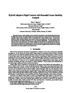
The experiments are conducted in an open-return low-speed wind tunnel having a square test section measuring 1m on the side. The present experiments use a 2-D airfoil model with a fixed cross section that is based on a NACA 4415 configuration as shown in figure 1. The chord length is c = 457mm, maximum thickness to chord ratio t/c = 0.15, and the model spans the entire width of the wind tunnel test section. The airfoil is modular and comprised of interchangeable spanwise segments which include a module of a circumferential array of 70 static pressure ports located at mid-span, and several modules of high-frequency integrated pressure sensors for measurements of instantaneous pressure. Bi-directional pitching moments induced by trapped vorticity flow-control are effected by individually-controlled miniature, hybrid surface actuators integrated with rectangular, high aspect ratio synthetic jets that are mounted on the pressure and suction surfaces near the trailing edge (Figure 1). The actuators have a characteristic height of 0.017c above the airfoil surface and the long dimension of the exit plane of each rectangular jet is parallel to the trailing edge and height (in the cross stream direction) of each jet orifice is 0.4 mm. The jets are generated by piezoelectric membranes that are built into a central cavity within the actuator and are operated off resonance within the range 1770Hz < fact < 2350Hz. The spanwise-segmented actuators are individually controlled from the laboratory computer and the system controller. The bulk of the present experiments are conducted at a free stream speed of U∞ = 30m/s, with a corresponding Reynolds number based on the airfoil chord length of Rec = 8.55 · 105 . At this speed, the actuation Strouhal number is St = fact c/U∞ = 34 and the maximum momentum coefficient is Cµ = 1 · 10−3 .
Figure 1. Render of wing model
In the present experiments, the wind tunnel model executes commanded flight maneuvers in two degrees of freedom (pitch and plunge) that are exclusively effected by flow control actuation within the constraints of the test section. The model is mounted on a programmable, 3-DOF (pitch, plunge, and roll) traverse that is constructed on an I-beam frame around the test section of the wind tunnel as shown in figure 2. The traverse is driven electromechanically by a dedicated feedback controller that removes the effect of parasitic mass and rotational inertia of the dynamic support system. The controller can also prescribe stability characteristics to mimic the behavior and control of a range of ”virtual” air vehicles, all having the same wing as the wind tunnel model, but with static margins that can be adjusted by the traverse controller, including unstable configurations for high maneuverability. The wing model is mounted on a rotating hollow shaft (which serves as conduit for wiring and pressure tubes). In one mode of operation pitch commands are executed by rotating the model using an AC servo
3 of 24 American Institute of Aeronautics and Astronautics
motor (torque motor) that is attached to one of the two vertical stages (figure 2) and is driven by a servo amplifier in torque mode to directly control the pitching moment on the model from the system’s controller (the pitch range is limited to ±25◦ ). At the opposite end the pitch shaft is supported by an air bearing that allows both rotational and axial motions. The axial motion allows the wind tunnel model to bank while it is maneuvered in pitch and plunge since the two plunge drives are controlled independently on each side of the tunnel. For open-outer-loop characterization the inner-loop controller is used to enforce a prescribed angle of attack α(t) trajectory. It also serves as a virtual variable tail surface by providing the torque required to trim the wing at any given condition, and by modifying its dynamic characteristics by changing its stiffness and damping properties. The application of torque T (α, α, ˙ α ¨ ) effectively alters ∂CM /∂α and ∂CM /∂ α˙ and the moment of inertia of the model, and allows for control of a range of stable and unstable configurations of “virtual” air vehicles. In addition, the servo motor is used as a transducer to indirectly measure the aerodynamic moment. In torque mode the motor generates a torque proportional to the input voltage and in steady state, the motor torque balances the aerodynamic moment, and moment due to gravity. Vertical (plunge) commands are executed by two independently-controlled and synchronized linear slides mounted vertically on opposite sides of the wind tunnel test section. As shown in Figure 2, the linear slide on the left carries the pitch axis drive mechanism and the slide on the right carries the air bearing. Both ends of the pitch axis are connected to the linear slides through gimbals that allow free rotation about axes in the streamwise and cross stream directions, and prevent misalignment from binding the plunge slides. Each slide includes a carriage that is moved along rails by a 20mm pitch ball screw turned by an AC servo motor with an integrated encoder and an electromagnetic release brake that prevents load on the carriage when the traverse is not in operation. The travel of each linear slide is constrained by adjustable stops and limit switches. The model shaft moves in plunge through vertical slots in the side walls of the test section. The controller synchronizes the motion of the linear drives and thereby can enable controlled plunge and roll of the model. A force sensor based on a spring set and load cell system and linear accelerometers allow for measurements of the vertical forces and compensation for the weight and inertia of the model. In the present work, the linear motion of the model is software limited to speeds and accelerations of up to 0.5m/sec and 2g, respectively (the maximum design speed and acceleration in the present configuration are 2.5m/sec and 5g).
Figure 2. Render of traverse showing various components
4 of 24 American Institute of Aeronautics and Astronautics
III.
Aerodynamic Model
A low-order vortex model for a pitching and plunging airfoil with trailing-edge synthetic jets was presented in Tchieu et. al. (2006)9 . In this section we review that model for the purposes of developing a control design model. Unlike many other low or reduced-order models, this model is built from physical principles, i.e. the conservation of momentum. The vorticity in the model consists of freely-moving vortices in the wake, a trapped control vortex with circulation ΓC (t), and the boundary-layer vorticity on the airfoil surface. We consider small-amplitude motions of a flat-plate airfoil which leads to a number of simplifying assumptions. Thus, for example, all but one of the wake vortices move uniformly downstream along the nominal x-axis that is fixed to the airfoil. The exception is the vortex being fed circulation from the trailing edge. The velocity of the latter vortex is modified to conserve momentum as discussed below. In addition we assume that vorticity is shed into the wake to satisfy the unsteady Kutta condition (no velocity singularity) at the trailing edge. Also, a vortex sheet with a continuous distribution of vorticity γ(x) is used to satisfy the boundary condition on the airfoil surface (normal component of velocity is continuous) plus the Kutta condition. For the control input, the synthetic jet is modeled with a trapped vortex that represents the averaged effect of the actuation. The control vortex circulation depends on the control variable, u, for example, dΓC = F (u, ΓC ). dt This function, F , can only be experimentally determined. III.A.
(2)
Wake Vortex Dynamics
Consider an airfoil of chord length c occupying the portion −c/2 ≤ x ≤ c/2 of the x-axis as presented in figure 3. The airfoil is undergoing small-amplitude motions in pitch and plunge. The pivot point for rotation is located at x = −a as shown. The airfoil velocity is U in the negative x-direction. Alternatively, one could apply the results below to a stationary airfoil with a freestream velocity U in the positive x-direction. See figure 3 where the fluid flow and the airfoil motion are given relative to a frame of reference moving in the negative x-direction with the airfoil. y U y˙ M(a) θ
1 0 0 1 − 2c
−a
c 2
Γ1
Γ2
...
Γi
1 0 0 1
1 0 0 1
1 0 0 1
1 0 0 1
ξ2
...
ξi
ξ1
x
Constant Strength Vortices Control Vortex, ΓC , ξC Nascent Vortex Figure 3. Pitching, plunging airfoil, control vortex with strength ΓC , and free wake vortices with strengths Γi , i = 1, ..., N.
Now also consider a wake vortex with circulation Γi located at x = ξi . This vortex will result in a given distribution of vorticity on the airfoil, γi (x), to satisfy the boundary condition on the airfoil and the Kutta condition given by (see, e.g., von Karman and Sears (1938)10 ) s s Γi c/2 − x ξi + c/2 γi (x) = . (3) π(ξi − x) c/2 + x ξi − c/2 5 of 24 American Institute of Aeronautics and Astronautics
We find that Z
"s
c/2
γi (x)dx = Γi −c/2
# ξi + c/2 −1 . ξi − c/2
(4)
It appears that the correct location of the control vortex should be slightly forward of the trailing edge and just above the airfoil for suction-side actuation and just below the airfoil for pressure-side actuation. The total effect of both actuators can be represented by a single vortex on the mid-plane located slightly forward of the trailing edge. In any event, the control vortex with strength ΓC will produce a corresponding contribution to the airfoil circulation given by γC (x). We assume that a change in ΓC on its own produces no net change of circulation in the wake. Thus, Z
c/2
γC (x)dx = −ΓC .
(5)
−c/2
The total circulation, which must equal 0, is therefore given by s N X ξi + c/2 = 0. Γ0 + Γi ξi − c/2 i=1
(6)
Here Γ0 is the quasisteady circulation about the airfoil that depends only on the pitch angle, its time derivative, and the plunge rate, and N is the number of free vortices in the wake. It is also assumed that all but one of the free vortices in the wake move with speed U . Thus, dξi = U (i ≥ 2), dt
(7)
and the vortex being fed circulation (labeled i = 1) moves with speed dξ1 (ξ 2 − c2 /4) dΓ1 =U− 1 dt ξ1 Γ1 dt
(8)
where we have used conservation of impulse to derive Eq. (8). This is in contrast with previous models where the force on the vortex and branch cut system was forced to be invariant.11–14 It has been found that this so-called Brown-Michael correction introduces the incorrect initial lift curve for the specific case of the flat-plate undergoing an impulsive start. The conservation of impulse argument given above, correctly captures the initial behavior for this specific case. Except for the vortex being fed, all vortices in the wake remain at constant circulation, i.e. dΓi = 0 (i ≥ 2). dt
(9)
The strength of Γ1 is such that Eq. (6) remains satisfied. As mentioned earlier, the circulation of the control vortex is given, for example, by dΓC = F (u, ΓC ), dt
(10)
where u is the control variable and the function f is to be determined. With the absence of a model for Eq. (10), Eqs. (6)-(9) constitute a close system of equations for the wake dynamics of the system given a sufficient initial condition. Since Eqs. (7) and (9) are easily integrable, this system can be reduced to one non-linear differential, i.e. Eq. (8), with the algebraic constraint represented by Eq. (6). In accordance to Eq. (1), the fluid states are represented by xf = [ξ1 Γ1 ]T . In contrast to other models, the fluid state is directly related to the physical variables of vortex location and strength.
6 of 24 American Institute of Aeronautics and Astronautics
III.B.
Lift and Moment Relationships
From the results derived in our previous work,9 we have the following expressions for the lift and moment. " # N c2 ac2 ¨ c ˙ U˙ c2 ρU c X Γi 2 p L = −ρπ( y¨ + U cy) − ρU ΓC , ˙ − ρπ θ + U (a + )cθ + ( + U c)θ − 4 4 2 4 2 i=1 ξi2 − c2 /4
(11)
and · 4 ¸ N ρπU c2 c ¨ U ac2 ˙ U 2 c2 ρU c2 X Γi p M (a) = aL + y˙ − ρπ θ− θ− θ + − ρU ΓC ξC , 2 4 128 4 4 8 i=1 ξi − c2 /4
(12)
The lift coefficient, defined as CL = 2L/(ρU c2 ), is " # N 2 c ac ¨ 2a + c ˙ cU˙ + 4U 2 2 1 X Γi p − CL = −π( 2 y¨ + y) ˙ −π θ + θ + ΓC , θ − 2 2 2 2 2U U 2U U 2U U i=1 ξi − c /4 U c
(13)
and the moment coefficient (with pitch up as positive) CM = −2M (a)/(ρU 2 c2 ) is
CM =
· 2 ¸ N π c ¨ a ˙ 1 1 X Γi 2ξC a p CL + y˙ − π θ − θ − θ + − ΓC . c 2U 64U 2 2U 2 4U i=1 ξi2 − c2 /4 U c2
(14)
The above equations can quite be integrated in time easily. Equation 8 is singular when t = 0. In general, a small-time, asymptotic solution is necessary to provide a sufficient initial condition for the startup of the simulation. This model uses a different strategy to determine ξ1 (t) and Γ1 (t). From the conservation of total circulation, Eq. (6), we can write s Γ1
N X ξ1 + c/2 = −Γ0 + Γi ξ1 − c/2 i=2
s ξi + c/2 ≡ G(t), ξi − c/2
(15)
where the newly defined function G(t) can be considered known up to time t. In addition, Eq. (8) can be written as d ( dt
q
ξ1 Γ1 U
ξ12 − c2 /4 Γ1 ) = p
ξ12
−
c2 /4
=
ξ1 GU . ξ1 + c/2
(16)
Defining q H(t) ≡
ξ12 − c2 /4 Γ1 ,
(17)
we can write Eq. (16) as H + cG/2 dH = GU, dt H + cG
(18)
where we have used Eqs. (15) and (17) to determine ξ1 as
ξ1 =
H + cG/2 . G
Similarly, Γ1 is found to be 7 of 24 American Institute of Aeronautics and Astronautics
(19)
r Γ1 = G
H . H + cG
(20)
WIth this approach, integrating equation (18) is numerically is now straightforward. Physically we expect that Γ1 (t) cannot decrease in magnitude as time progresses. Let t∗ be a time when dΓ1 /dt changes sign. Thus we check, after each time increment, to see if Γ1 has decreased in magnitude. If so, we return to the previous time t, which, by definition, t = t∗ , and add the present Γ1 and ξ1 to the list of wake vortices labeled i ≥ 2 and form a new i = 1 vortex with initial conditions ξ1 (t∗ ) = c/2 and Γ1 (t∗ ) =p 0. Typically, near t ≈ t∗ (t > t∗ ) we expect G ∼ t − t∗ which leads to ξ1 ≈ 1 + U (t − t∗ )/4 and Γ1 ≈ G(t) U (t − t∗ )/8 for U (t − t∗ ) ¿ 1. An exception to this behavior would occur, for example, p for an impulsive start at t = 0 with say G(0) = −Γ0 (0) 6= 0. In this case, ξ1 ≈ 1 + U t/2 and Γ1 ≈ −Γ0 (0) U t/4 for U (t − t∗ ) ¿ 1. III.C.
Rigid-Body Dynamics
Dealing with the fluid and body interaction problem is usually a difficult problem. For this case, due to the low-order fluid model, a closed system of equations can be constructed to predict the orientation and the motion of the airfoil. To model an airfoil is free flight it is assumed that the airfoil is attached to a spring and damper in the y-direction in addition to a torsional spring and damper in the θ-direction. This stabilizes the system and gives a model for non-stalled flutter in cross-flow.15 The system of equations for the airfoil in this configuration becomes m¨ y − Sx θ¨ + by y˙ + ky y I θ¨ − Sx y¨ + bθ θ˙ + kθ y
=
L
=
M (a)
U
ky
by
(21)
where L is the lift, M (a) is the moment about the location a, Sx is the static imbalance per unit width, and all other terms are related to the linear and rotational mass, damping, and stiffness of the system.b The static imbalance per unit width is defined as Z Sx ≡ ξρs dξdη This is an area integral in a principle coordinate system where ρs is the density of the structure, and ξ and η are the principle coordinates. This can equivalently be expressed as
Γ1 bθ
kθ
1 0 0 1 ΓC , ξ C
1 0 0 1 ξ1
Figure 4. Schematic showing the configuration of rigid body coupling. Here the rigid body is attached to a mass-damperspring system in both the plunge and pitching degrees of freedom. See figure 3 for more detail.
Sx = ma where m is the mass of the object and a is the distance from the elastic axis (the point at which the springs and dampers are attached) to the center of mass, previously defined in figure 3. III.D.
Non-zero Thickness and Camber Correction
This model assumes that the wing is a flat plate. To correct the neglected effect of thickness and camber on the lift and moment, we introduce corrections to the lift coefficient and moment coefficients in Eqs. (13) and (14). It is believed that the corrections are static and do not depend on the angle of attack in the range of operation or the unsteady maneuvering. Thus we simply add the the zero angle of attack lift and moment coefficient to obtain C˜L = CL,0 + CL C˜M = CM,0 + CM b Note
that a right hand system has been used in this case, thus positive θ (or moment) corresponds to pitch down.
8 of 24 American Institute of Aeronautics and Astronautics
For example, on a clean NACA 4415 airfoil, the moment coefficient is nearly constant through the quarter chord for the range of angle of attacks in this study and thus CM,0 ≈ −0.1.16 For the lift coefficient, the change in lift per angle of attack for the NACA 4415 is nearly that of a flat plate and thus we correct the lift by offsetting the lift coefficient by the zero angle of attack lift for a NACA 4415, i.e. CL,0 ≈ 0.4. Of course, this correction is wing section dependent and is taken from experimental results. This results in the following lift and moment corrections. µ ¶ ˜ = L + 1 ρU 2 c CL,0 L 2 µ ¶ ¶ ³ ´ µ1 ˜ = M − 1 ρU 2 c2 CM,0 + a − c M ρU 2 c CL,0 2 4 2 ¡ ¢ In our experiments, the c.g. is close to quarter chord and M simplifies since a − 4c ≈ 0.
IV.
Control Formulation
Though the developed model is a set of ordinary differential equations, it cannot be used for control design. Due to the highly nonlinear manner in which a vortex is added, the model is not casual. If the error caused by not resetting the time step in the model is neglected, the model can be made casual. However, because a vortex is created at each time the nascent vortex strength changes sign, at which point, the model resets the fluid dynamic states, i.e. it resets the location of the vortex at ξc = c/2 and the corresponding strength to ΓC = 0. This is a result of the low-order nature of the model. While in this model the number of model states are kept fixed, in reality the number of vortices ultimately increases. To circumvent this problem the previous states are reused for the newest vortex. This causes a discontinuity in both the vortex position and strength when a new vortex is shed. IV.A.
A Simplified Control Design Model
The vortex model by its nature captures some dynamics that negligible on the time scales of a flight control system. From this prospective, it is reasonable to expect that it is possible to simplify the model further to make it appropriate for control design. When examining the lift and moment equations, (11) and (12), we observe that it is a function of only the states of the rigid body (i.e. both the added mass and the quasi-steady terms) in addition to a term due to the wake. For example, consider the lift equation. In this case, the term due to the wake is simply N
LW
ρU c X Γi p =− 2 i=1 ξi2 − c2 /4
(22)
Therefore, we define a characteristic circulation for the entire wake as ΓW = c
N X i=1
Γi
p
ξi2
− c2 /4
(23)
Even though the discontinuities of the flow (i.e. the startup of Γi and ξi ) are included in this term, ΓW is fairly smooth. Hence, its reasonable to model this term using an ordinary differential equation. To choose a satisfactory differential equation, examine the startup case where dΓw /dt = 0 and only a single vortex is created. In this case ¶ µ 1 (24) L = −ρU Γ0 + ΓW 2 From classical theory, it is expected that half of the lift is attained at the moment the plate is impulsively started from rest. Thus, at t = t0 , ΓW ≈ −Γ0 . When t → ∞, the lift term due to the wake term should disappear as the wake vortices move further and further away. Therefore we propose using the model dΓ0 dΓW =− − βΓW dt dt 9 of 24 American Institute of Aeronautics and Astronautics
(25)
where β is a constant. Note that this introduces an exponential decay of ΓW (which gives a 1 − eβt rise in lift) given a constant Γ0 . This is contrary to the classical square root type growth for the lift and a decay in the lift that is geometric at best. We choose β to best fit the case of an impulsive start flat plate by computing a norm between the original model and the simple model. The best fit for a given ∆t = T is given in table 1. We chose β = 0.406. T 20 10 5
β 0.333 0.360 0.406
Table 1. Best fit for β
From this, a linear model can be formed consisting of geometrical parameters and the derivatives of y and θ. The differential equation governing the fluid dynamics reduces to a simple first order differential equation ´ ³ ³ c´ ¨ θ + U θ˙ Γ˙ W + βΓW = −πc y¨ + a + (26) 4 with an initial condition of
h ³ i c´ ˙ ΓW (t0 ) = −πc y˙ + a + θ + Uθ 4 t=t0
(27)
Furthermore, the lift and moment expressions simplify to: " Ã ! # ¶ µ 2 ³ U˙ c2 ρU ac2 ¨ c´ ˙ c 2 y¨ + U cy˙ − ρπ θ+U a+ cθ + +U c θ − ΓW − ρU ΓC L = −ρπ 4 4 2 4 2
(28)
and · 2 ¸ ρπU c2 ac ¨ U ac2 ˙ U 2 c2 ρU c M = aL + y˙ − ρπ θ− θ− θ + ΓW − ρU ΓC ξC 4 128 4 4 8
(29)
The above equations include added mass, quasi-steady lift, lift due to wake, and control terms.
V.
Linear Control Formulation
For control design is desirable to rewrite the simplified equations of motion as a matrix quadruple. To this end, we can equate equations (28), (29), and (21) to form the rigid body differential equations as " # " # " # y¨ y˙ y (30) M +D +K + AΓw = BΓc θ¨ θ˙ θ where the mass matrix M is given by " M=
2
2
m + ρπc 4 2 −Sx + aρπc 4
−Sx + ρπ ac4 2 c4 I + aρπ ac4 + ρπ 128
# (31)
the stiffness matrix is given by K=
³ ky
ρ ³
U˙ c2 4
´ + U 2c
´ − aU 2 c
(32)
# ¢ ¡ by + ρπU c ρπU a + 2c c ¡ ¢ ¡ ¢ ρπc aU − U4c bθ + aρπU a + 4c
(33)
0
kθ − ρπ
U 2 c2 4
−
aU˙ c2 4
the damping matrix is given by " D=
10 of 24 American Institute of Aeronautics and Astronautics
and the aerodynamics coupling matrix, A, and the control matrix, B, is given by " # " # ρU −ρU 2 ¡ ¢ , B= A= ρU a2 − 8c −ρU (ξc + a)
(34)
The governing relation for aerodynamics in equation (26) combined with (30) is used to form the required matrix quadruple ¯x + BΓ ¯ c x ¯˙ = A¯ ¯ ¯ y = Cx ¯ + DΓc
(35)
where the system state, x ¯ = [y θ y˙ θ˙ Γw ]T and
0 −1 ¯ −M K A= £ ¡ ¢¤ c πc 1 + a + 4 M −1 K
I −M −1 D h £ ¡ ¢¤ πc 1 + a + 4c M −1 D − 0
0 −M −1 A (36) i £ ¡ ¢¤ πc 1 + a + 4c M −1 A − β πcU
and ¯= B
0
C¯ =
M B , ¢¤ £ ¡ c −1 −πc 1 + a + 4 M B −1
1 0 0 0
0 1 0 0
0 0 1 0
0 0 0 1
0 0 0 0
,
D=
0 0 0 0
(37)
Note that the control term ΓC is a non-physical variable that is related to control voltage and the system states. This relationship will be explored in more detail later in the paper. Also, not all of the states are measurable. If all of the states were measurable, it is easy to formulate a control design based on LQR theory. In this paper, the nominal control design consists of a robust servomechanism LQR control law with augmented feed forward term to improve transient error tracking response. Consider the linear time invariant state space model: x˙ = F x + Gu + Ew y = Hx
(38)
where x²Rn , u²Rm , w²Rm and y²Rl . Furthermore, it is assumed that w is an unmeasurable disturbance. Next we define the command input vector r²Rp such that r satisfies the differential equation given in 39 and we assume that the disturbance w satisfies the same differential equation. r(p) =
p X
ai r(p−i)
(39)
i=1
Assuming that the p < l and defining the error signal as: e=y−r
(40)
and given the control objective that the command error e(t) → 0 as t → ∞ in the presence of unmeasured disturbances satisfying 39, it is possible design an optimal stabilizing control law for the plant dynamics given in 38. The solution of this standard formulation is derived in Wise17 and yields that nominal control signal of the form: Z t (41) u = −Ke e(τ )dτ − Kx x 0
Letting r satisfy r˙ = 0, the LQR based technique yields an integral action on the tracking error that allows for robust tracking of commands with zero steady state error. Augmenting the control law in 41 with 11 of 24 American Institute of Aeronautics and Astronautics
a feedforward term, Z, and allowing for an additional augmenting control input, ∆u, for adaptive control design the final nominal control law is given by: Z t u = −Ke e(τ )dτ − Kx x + Zr + ∆u (42) 0
Graphically this can be represented as the simulation diagram shown in figure 5. The effect of the feedforward term is to help speed up the transient response of the control law. From a frequency domain standpoint, the eigenvalues of the closed loop system remain fixed under a constant gain Z. In a SISO system, this is equivalent to adding an adjustable zero that allows the designer to cancel a slow pole in closed loop transfer (s) function YR(s) .
Figure 5. Robust Servo LQR with feedforward element and added control signal
Since the system is not full state feedback, we use the static projective control technique17 , to formulate an output feedback law without feedback of the flow state. Augmenting the model dynamics with the control law dynamics, the closed loop system is given by " # " #" R # " # e 0 Ct e −1 = + r ¯ e A¯ − BK ¯ X ¯ x˙ −BK x BZ " # h i e yt = 0 Ct x where Ct is a matrix that multiplied by x that gives the plunge position, z. Since, we are not using the flow state in feedback we can retain all but two of the closed loop eigenvalues. Let K = [Ke Kx ] and Xy be the eigenvectors corresponding to the closed loop eigenvalues we wish to retain. Then the required output feedback gain is computed as ¡ ¢ ¯ = KXy C¯meas Xy −1 K R ˙ T . The where C¯meas corresponds to measured states of x such that ymeas = C¯meas x = [ e y θ y˙ θ] projective control effort is then defined by " # R e ¯ Γ C = −K + Zr ymeasured Though this technique does not guarantee closed loop stability, in practice, closed loop stability is easily satisfied. V.A.
Augmenting Output Feedback Adaptive Control
The assumed linear dynamics of the model (35) ignores nonlinearities and unmodeled dynamics associated with the flow actuation process. We assume that the true dynamics of the system can be represented as: ¯ + BΛ ¯ (Γc + f (x, Γc )) x˙ = Ax y = Cx 12 of 24 American Institute of Aeronautics and Astronautics
(43)
where C is a matrix capturing the the system output, A ∈ Rnxn , B ∈ Rnxm , and C ∈ Rmxn are known matrices. Λ ∈ Rmxm is an unknown but constant positive definite matrix, x ∈ Rn is the system state, u ∈ Rm is the control input, y ∈ Rm is the system output, and f : Rn × Rm 7→ Rm is Lipschitz continuous function that is unknown. The nominal vortex control law has the form ΓC,n = −Ky y + Kr r
(44)
where Ky ∈ Rmxm and Kr ∈ Rmxr where chosen such that the following reference system achieves the desired tracking characteristics x˙ m (t) = Am xm (t) + Bm r ym (t) = Cxm (t)
(45)
where Am = A − BKr is Hurwitz and Bm = BKr . For the purposes of adaptive design, assume that Am satisfies the following Lyapunov equation ATm P + P Am = −Q,
Q = QT > 0,
Q ∈ Rnxn
(46)
To introduce an adaptive signal to compensate for f (x, Γc ), we redefine the total control effort as (47)
ΓC (t) = ΓC,n (t) − ΓC,ad (t)
Inserting the control law given in (42) into the open loop dynamics (43) the closed loop dynamics can be written "
# e˙ x˙
" =
#" 0 ¯ −BKI
C ¯ ¯ X A − BK
# e x
" +
# −1 ¯ BZ
" r+
# 0 ¯ B
(−uad + ∆ (x, xa , Γc ))
x˙a = g (x, xa , Γc ) " # h i e y= 0 C x
(48)
One can rewrite the closed loop system in a more compact form as x(t) ˙ = Am x(t) + Bm r + B [δΛΓC (t) + Λf (x, ΓC ) − ΓC,ad ]
(49)
We wish to approximate Λf (x, ΓC ) by a nonlinear in parameters neural network. To construct such an approximation in an output feedback setting18–22 , we reconstruct the system states via delayed values of system outputs and inputs. If the number of delayed values for each output is s, the number of delayed values for each input is t, and the length of the time delay time is d, the delayed value vector, η(t), is given by η(t) = [[y1 (t), y1 (t − d), ..., y1 (t − sd), ..., ym (t), ym (t − d), ..., ym (t − sd)]T ; [ΓC,1 (t − d), ..., ΓC,1 (t − sd), ..., ΓC, m(t − d), ..., ΓC,m (t − sd)]T ]
(50)
where η(t) ∈ Rw and w = (s + t)m. Note that the current control output is not included in η(t). This is prevent to implementation issues associated with realizing the control. Using η(t), we assume that the function f (x, ΓC ) can be approximated over a compact set Dx × DΓC to an arbitrary degree of accuracy such that Λf (x, ΓC ) = W T σ ¯ (V T η(t)) + ²(x, ΓC ),
(x, ΓC ) ∈ Dx × DΓC
(51)
where k²(x, ΓC )k < ²∗ < ∞, σ ¯ (q) = [1, σ1 (q1 ), · · · , σ1 (ql )], l is the number of hidden layer neurons, 1 and W ∈ R(l+1)xm and V ∈ Rwxl are unknown but constant neural network ideal weights. σi (z) = 1+exp(−z) The closed loop system can then be equivalently expressed as £ ¤ (52) x(t) ˙ = Am x(t) + Bm r + B δΛΓC (t) + W T σ ¯ (V T η(t)) − ΓC,ad + B²(x, ΓC ) 13 of 24 American Institute of Aeronautics and Astronautics
To develop the complete output feedback algorithm, an error observer must be introduced. Consider the following error observer ξ˙ = Am ξ + L(y − yξ − ym ) yξ = Cξ
(53)
such that A˜ = Am − LC is Hurwitz and satisfies the following Lyapunov equation ˜ A˜T P˜ + P˜ A˜ = −Q,
˜=Q ˜ T > 0, Q
˜ ∈ Rnxn Q
(54)
The adaptive control signal is given as h i−1 h ³ ´i ˆ ˆ n+W ˆ Tσ uad = Im + δΛ δΛu ¯ Vˆ T η(t)
(55)
The adaptive update laws are defined as ´ i ³ h ˆ (t), σ ˆ˙ (t) = −ΓW P roj W ˜ Vˆ (t), η(t) ξ(t)T P B W h ³ ´i ˙ ˆ (t), Vˆ (t), η(t) Vˆ (t) = −ΓV P roj Vˆ (t), η(t)ξ T P BH W h T i ˆ˙ T (t) = −Γδ P roj δΛ ˆ (t), u(t)ξ T (t)P B δΛ where
³ ´ ³ ´ ³ ´ σ ˜ Vˆ (t), η(t) = σ ¯ Vˆ (t)T η(t) − σ ¯ 0 Vˆ (t), η(t) Vˆ T (t)η(t) ³ ´ ³ ´ ˆ (t), Vˆ (t), η(t) = W ˆ T (t)¯ H W σ 0 Vˆ (t), η(t)
(56)
(57)
and ´ ³ σ ¯ 0 Vˆ (t), η(t) =
0 dσ1 (dq1 (t)) dq
.. . 0
··· ··· .. . ···
0 0 .. .
(58)
dσl (dql (t)) dq
where qi is the ith row of q = Vˆ (t)T η(t). Its easy to show with a standard Lyapunov candidate that the adaptive weights are bounded and that the system tracking error is uniformly ultimately bounded. The modeling error f (x, Γc ) is a function of unmodeled flow dynamics as well. In the absence of an analytical model for flow actuation dynamics and devices to measure the related states, we can only use measurable states in the adaptive controller. In the relatively low bandwidth maneuvers performed in our experiments, the effects of flow dynamics on rigid body dynamics are expected to be small. In addition, we also assume that such effects are observable from rigid body states. With these assumptions, the adaptive signal defined in 55 can be used to approximate f (x, Γc ). V.B.
Control Hedging
In order to prevent adaptation to effects due to control saturation control hedging has been applied to modify the reference model (45). The difference between the commanded control and the control applied to the plant is defined as the hedge signal. The hedge signal is then subtracted from the input to the plant model of the reference model as shown in figure V.B. This modification effectively moves the reference model backwards by an estimate of the amount the controlled system did not move due to saturation and produces a reachable command within the capabilities of actuation. With this modification during periods of full saturation tracking error remains small, preventing winding up of the NN weights. Applying control hedging to the adaptive vortex control algorithm in this paper requires the hedging algorithm to be gain scheduled. The reference model is modified as x˙ m = Am xm + Bm r + Bh ΓC,h 14 of 24 American Institute of Aeronautics and Astronautics
where Bh is the modeled control effectiveness matrix. The hedge signal is computed as ΓC,h = g(uf , θ) − ΓC where g(uf , θ) models the saturation limits of the actuator and ΓC is the ideal control action. This is illustrated graphically in figure V.B and the actuator model, g(uf , θ) is shown in figure V.B.
� � � �������
� �����
�������� �
� � � �������
� ��� ��
�� �
� � � ��� ��
�� � � ��
Figure 6. Control Hedging diagram.
0.5 0.4 0.3 0.2 Maximum ΓC
Γ
C
0.1
�
�
Minimum ΓC
0 −0.1 −0.2 −0.3 −0.4 −15
−10
−5
0
θ (deg)
5
10
15
20
Figure 7. Gain scheduled saturation block.
VI.
Model and Control Design Validation
Experimental verification of the model was performed under open loop excitation.9 Numerical simulations were also used to validate the models in situations not realizable by the experiments. The numerical
15 of 24 American Institute of Aeronautics and Astronautics
simulations were computed at the University of Texas at Austin using a Delayed Detached Eddy Simulation (DDES). The DDES scheme is a hybrid non-zonal Reynolds-Averaged Navier-Stokes (RANS) and LargeEddy Simulation (LES) turbulence model based on the Detached Eddy Simulation (DES) model. Simulations were run at a free-stream Reynolds number, Re = 9 × 10⁵ . In this section, the model developed in our previous research was used to validate control design effort under high bandwidth free flight conditions and wind tunnel experiments conducted on a novel traverse capable of simulating free flight was used to further validate the control algorithms. VI.A.
Experimental Determination of Control Vortex Strength vs. Actuator Input Voltage
In the development of the control law, the control input was assumed to be Γc . In reality, a control moment is generated via a continuous signal (DC voltage) representing a commanded change amplitude modulation. The effect is analogous to a commanded control surface deflection in conventional flight control. Positive control signal indicates nose up moment and requires activation of the pressure side (PS) actuators and similarly negative control signal requires activation of the suction side (SS) actuators. Alternate amplitudemodulated operation of SS (top) and PS (bottom) actuators with a sample control signal is shown in figure 8.
Figure 8. Amplitude Modulated Flow Actuation
It has been previously shown that the usage of synthetic jets traps vorticity in the boundary layer to directly modify the flow in the average sense.4, 23 This can be also be viewed as “virtual shaping” of the airfoil since this modifies the streamlines in the vicinity of the actuator. Here we model this “virtual shaping” or trapped vorticity as a stationary control vortex that depends on the control parameter (e.g. voltage), u. Since the PS and SS actuation do not act at the same time, the control vortex can be thought of as one vortex (situated on the x-axis) with a positive strength representing PS actuation and a negative strength representing SS actuation. Experiments show that the pressure distribution away from the neighborhood of the actuation point is essentially unaffected. This leads to the conclusion that no net circulation is injected into the wake as a direct consequence of turning the actuation on or off. For simplicity, we model the actuation with a single vortex located on the x-axis. If the time scale for formation of ΓC