Wave based calculation methods for sound-structure interaction ...

Arenberg Doctoral School of Science, Engineering & Technology Faculty of Engineering Department of Civil Engineering

WAVE BASED CALCULATION METHODS FOR SOUND-STRUCTURE INTERACTION APPLICATION TO SOUND INSULATION AND SOUND RADIATION OF COMPOSITE WALLS AND FLOORS

Promotor: Prof. dr. ir. G. VERMEIR

Dissertation presented in partial fulfillment of the requirements for the degree of Doctor in Engineering by

Arne DIJCKMANS

June 2011

WAVE BASED CALCULATION METHODS FOR SOUND-STRUCTURE INTERACTION APPLICATION TO SOUND INSULATION AND SOUND RADIATION OF COMPOSITE WALLS AND FLOORS

Jury: Prof. dr. ir. P. Van Houtte, chair Prof. dr. ir. G. Vermeir, promotor Prof. dr. ir. W. Desmet Prof. dr. C. Glorieux Prof. dr. ir. G. Lombaert Prof. ir. E. Gerretsen (TU/e, Nederland) Prof. dr. rer. nat. M. Vorländer (RWTH Aachen)

Dissertation presented in partial fulfillment of the requirements for the degree of Doctor in Engineering by

Arne DIJCKMANS

June 2011

c 2011 Katholieke Universiteit Leuven, Groep Wetenschap & Tech nologie, Arenberg Doctoraatsschool, W. de Croylaan 6, 3001 Heverlee, België Alle rechten voorbehouden. Niets uit deze uitgave mag worden vermenigvuldigd en/of openbaar gemaakt worden door middel van druk, fotokopie, microfilm, elektronisch of op welke andere wijze ook zonder voorafgaandelijke schriftelijke toestemming van de uitgever. All rights reserved. No part of the publication may be reproduced in any form by print, photoprint, microfilm, electronic or any other means without written permission from the publisher. D/2011/7515/78 ISBN 978-94-6018-376-8

Voorwoord Met het schrijven van deze laatste woorden wordt een hoofdstuk uit mijn leven afgesloten. Een hoofdstuk waar ik met plezier naar terugkijk, mede dankzij een aantal mensen die hebben meegeholpen om deze uitdaging tot een goed einde te brengen. In de eerste plaats wil ik mijn promotor, professor Vermeir bedanken voor de steun en het vertrouwen, die ik de voorbije vier jaren heb gekregen. Hij heeft me ge¨ıntroduceerd in de interessante wereld van de bouwakoestiek - een wereld die twee van mijn jeugdige interesses samenbrengt, de architectuur/bouwkunst en de fysica. Hij gaf me de nodige ruimte om me wetenschappelijk uit te leven in deze wereld, maar ook de juiste sturing en motivatie met zijn inzicht en interesse. Furthermore I would like to thank the members of the jury for their participation in the jury and their careful evaluation of this work. Verder gaan mijn gedachten uit naar mijn copromotor, prof. Lauriks. Zijn onverwachte overlijden was een grote schok voor iedereen in de afdeling. Walter, ik vind het jammer dat je er niet meer bij bent. Hierbij dank ik het Fonds voor Wetenschappelijk Onderzoek Vlaanderen (FWO) voor het financieel ondersteunen van mijn onderzoek. Als ik terugblik, mag ik zeker de collega’s van de afdeling Akoestiek en Thermische Fysica niet vergeten. Zowel op als naast het werk is gebleken dat ingenieurs en fysici het (verbazend) goed kunnen vinden. Het was een fijne tijd! Tot slot wil ik mijn familie en vrienden bedanken voor de niet aflatende steun en interesse. Bedankt, iedereen, voor de verkwikkende momenten. Ma, pa, Inge, Wouter en kleine Rube, jullie wisten misschien niet altijd even goed waar ik mee bezig was, maar bedankt voor alles, om mij altijd ten gepaste tijde te hebben verstrooid, om mij te helpen uitkijken naar wat hierna komt.

I

II

Abstract In building acoustics, reliable prediction methods for sound transmission and sound radiation are required for parameter studies, material selection and optimization studies. Today there is a lack of calculation techniques which can be used in the entire frequency range of interest. Therefore a numerical prediction tool for building acoustical purposes has been developed in this work. It can be used in a broad frequency range to simulate direct sound transmission through finite-sized, composite walls and floors. The model is based on the wave based method for the acoustic domains and a modal approach to describe the structural response. To model multilayered structures consisting of elastic and poro-elastic layers, the wave based method is combined with the transfer matrix method in a new hybrid model. The full room-structure-room description allows reliable predictions in the low-frequency range. The enhanced computational efficiency of the wave based method compared to finite element models allows calculations at higher frequencies. The model is validated with airborne and structure-borne sound insulation measurements and used to investigate the repeatability and reproducibility of sound insulation measurements in the low- and mid-frequency range. Results focus on the influence of finite dimensions on sound transmission loss of composite structures and the relative importance of source and receiving room. Based on the model, the understanding of sound transmission through lightweight double walls and multilayered structures with air layers is improved. Wave based simulations show the importance of cavity absorption and the vibro-acoustic coupling between plate and cavity modes. Furthermore, experiments and simulations have demonstrated that friction and viscous effects have a very significant influence when thin air layers are involved in sound transmission.

III

IV

Beknopte samenvatting Binnen de bouwakoestiek is de ontwikkeling van betrouwbare rekenmodellen nuttig voor parameterstudies, materiaalselectie en optimalisatie van de akoestische eigenschappen van bouwelementen. Momenteel is er een gebrek aan rekenmethoden die in het hele bouwakoestische frequentiegebied inzetbaar zijn. Daarom is in dit werk een numeriek model ontwikkeld dat gebruikt kan worden om de directe geluidtransmissie doorheen samengestelde wanden en vloeren met eindige afmetingen te voorspellen in een breed frequentiegebied. Het model is gebaseerd op de golfgebaseerde methode voor de akoestische respons en een modale expansietechniek voor de structurele verplaatsingen. Om meerlaagse structuren, bestaande uit elastische en poro-elastische materialen, te modelleren is de golfgebaseerde methode gecombineerd met de transfer matrix methode in een nieuw hybride model. De volledige beschrijving van het kamer-structuur-kamer probleem laat betrouwbare voorspellingen toe in het laagfrequente gebied. De verhoogde rekenkundige efficiëntie van de golfgebaseerde methode - vergeleken met eindige elementen modellen - maakt berekeningen mogelijk bij hogere frequenties. Het model is gevalideerd met lucht- en contactgeluidisolatiemetingen en gebruikt om de herhaalbaarheid en reproduceerbaarheid van geluidisolatiemetingen in het lage en middenfrequentiegebied te onderzoeken. De invloed van eindige afmetingen op de geluidisolatie van samengestelde structuren en het relatieve belang van zenden ontvangruimte wordt getoond. Het model heeft een beter inzicht gegeven in de geluidtransmissie doorheen lichte dubbele wanden en meerlaagse structuren met luchtlagen. Golfgebaseerde simulaties tonen het belang van spouwabsorptie en van de vibro-akoestische koppeling tussen plaat- en spouwmodes. Verder hebben experimenten en simulaties ook aangetoond dat viskeuze effecten en wrijving een zeer bepalend effect hebben wanneer dunne tussenliggende luchtlagen in de geluidtransmissie betrokken zijn.

V

VI

List of symbols Abbreviations 1D 2D 3D BEM EEM EPS FEM FRF GBM ISO SEA PMMA SPL STL TMM WBM WB-TMM

: : : : : : : : : : : : : : : : :

one dimensional two dimensional three dimensional boundary element method eindige elementen methode expanded polystyrene finite element method frequency response function golfgebaseerde methode international organization for standardization statistical energy analysis polymethyl methacrylate sound pressure level sound transmission loss transfer matrix method wave based method wave based - transfer matrix method

Arabic symbols atr A A0

: truncation factor : total absorption : reference value of total absorption (= 10 m2 )

VII

[m2 ] [m2 ]

List of symbols

Apq B0 c ca cn Cα

: : : : : :

contribution factor of plate mode plate bending stiffness sound velocity sound velocity in air contribution factor of wave function cavity absorption parameter

(ij) Cmn

: : : : : : : : : : : : : : : : : : : : : : : : : : : : :

wave based model auxiliary coefficient layer thickness distance Young’s modulus complex Young’s modulus frequency critical frequency mass-spring-mass resonance frequency force acoustic source function coefficient shear modulus complex shear modulus Gaussian distribution function plate thickness rigidity parameter (orthotropic plates) velocity transfer function sound intensity interface matrix √ imaginary unit (= −1) interface matrix wave number wave number in air bending wave number bulk modulus complex effective bulk modulus length sound intensity level normalized impact sound level sound pressure level

d d E E f fc fmsm F Fmn G G G(θ) h H0 Hv I I j J k ka kB K ˜ K L LI Ln Lp

VIII

[N m] [m/s] [m/s] [-]

[m] [m] [N/m2 ] [N/m2 ] [Hz] [Hz] [Hz] [N ] [N/m2 ] [N/m2 ] [m] [N m] [-] [W/m2 ]

[1/m] [1/m] [1/m] [N/m2 ] [N/m2 ] [m] [dB] [dB] [dB]

List of symbols

LW m00 Mp n

: : : :

sound power level surface mass plate bending moment per unit width normal direction

N (i) NV Nmn p p0 pˆs Pr Pmn , Qmn

: : : : : : : :

number of wave functions in domain i number of subdomains in wave based model norm of wave function ϕmn acoustic pressure reference sound pressure (= 2·10−5 P a) particular pressure solution Prandtl number of air contribution factors of room wave functions

i j Pmnpq q Q Qp

: : : :

~r rrev Rs R Rw S s00 t T Ts [T f ] [T p ] [T s ] u, v, w v V Vp

: : : : : : : : : : : : : : : : :

room-plate projection coefficient acoustic volume velocity distribution volume velocity plate transverse shear force per unit width position vector critical distance plane wave reflection coefficient sound reduction index weighted sound reduction index surface area dynamic stiffness time reverberation time plane wave transmission coefficient transfer matrix of a fluid layer transfer matrix of a poro-elastic layer transfer matrix of an elastic layer displacements velocity volume plate generalized shear force per unit width

(r p )

[dB] [kg/m2 ] [N m]

[P a] [P a] [-]

[1/s] [m3 /s] [N ]

[m] [-] [dB] [dB] [m2 ] [P a/m] [s] [s] [-]

[m] [m/s] [m3 ] [N ]

IX

List of symbols

W Winc Wtr x, y, z X, Y, Z Y Z Zc Zp Zs

: : : : : : : : : :

power incident sound power transmitted sound power local coordinate system global coordinate system mobility acoustic impedance characteristic impedance mechanical impedance surface impedance

[W ] [W ] [W ]

[m/N s] [N s/m3 ] [N s/m3 ] [N s/m3 ] [N s/m3 ]

Greek symbols α α α∞ γ δ η θ λ Λ Λ0 µ ν ρ ρa ρ ˜ σ σ σ τ τd φ φp

X

: : : : : : : : : : : : : : : : : : : : : :

absorption coefficient propagation constant tortuosity specific heat ratio of fluid Dirac function loss factor angle of incidence wavelength characteristic viscous length characteristic thermal length dynamic viscosity of fluid Poisson ratio density density of air complex effective density radiation factor flow resistivity stress transmission coefficient diffuse field transmission coefficient porosity plate rotation

[-] [1/m] [-] [-] [-] [◦ ] [m] [m] [m] [-] [-] [kg/m3 ] [kg/m3 ] [kg/m3 ] [-] [N s/m4 ] [N/m2 ] [-] [-] [-] [-]

List of symbols

ϕ ϕ ϕp ω Ω ΩI Ωp Ωw ΩZ

azimuth angle [◦ ] acoustic wave function plate wave function circular frequency [rad/s] boundary surface of cavity interface surface between two volume domains boundary surface with pressure boundary condition : boundary surface with normal displacement boundary condition : boundary surface with normal impedance boundary condition : : : : : : :

Miscellaneous symbols +-. IBP

40

30

20

10 63

125

f [Hz]

250

500

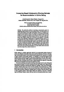
nes were applied according to the specFigure Figure 1.1: Sound transmission measuredat loss of a window with 6(16)6 mm 5. Soundreductionindex four laboratorieswitb -3. panes, measured at four laboratories with ISO 140 (from Pedersen ISO 140. Averagefor two paths of a moving loudspeaker x two time of reverberant receiving rooms was rotatingmicrophonesin eachroom.Windowwith 6-I6-6mm panes. et al. [2000]). g to ISO 140-3, but with an enlarged obtained with several loudspeaker and . -+-DELTA and but also on··.··PTB the dimensions of both the d pressure level at the test object waswall material properties - .• - CSTB - ->+-. IBP wall and the adjacent rooms. Therefore, a fundamental understanding rce room side for 12 fixed microphone 40 istributed over the entire surface of of the the sound-structure interaction and the influence of finite dimensions of rooms and structure on this interaction is essential for sound nce between test object and microphone transmission and sound radiation problems. The problem of calculat. For each microphone position the in30 the sound transmission and sound radiation of composite structures t least 30 s. Further, if a moving ing loudalso important in the automotive and aerospace industries and for the integration time covered a is whole

other noise control applications. In this context, a novel prediction tool

om the radiated normal intensityhas from been developed to analyze the sound-structure interaction between 20 easured as an average for horizontal and and composite building structures, like double walls or sandwich rooms erns as described in ISO/FDIS 15186-1. plates, in a broad frequency range. was steady and within the range 0.110 each scan was at least 60 s. Further, 250 125 63 500 f [Hz] ker was applied, the time of each1.2 scan State-of-the-art ber oftraverses. The accepted difference the 6. geometry, three basicindex approaches emFigure Intensity sound reduction measured atare four commonly laboranormal intensity level for the twoRegarding scans ployed in torieswith analysisnewtechniqueof of sound transmission problems. (i) The first apmeasurement.Absorbingback-wallsin receiving Averagefor two paths of of ainfinite moving loudspeaker. proach ofrooms. considering structures lateral dimensions. alls were obtained with for example a consists Source room measurementclose to test object. Windowwith 6-16(ii) In a second view a finite-sized structure is placed in an infinite yer of mineral wool with a specific flow 6mmpanes. rigid mately 10 kPa s/m2 . It is by theory pos-baffle, so finite sizes of the structure are accounted for. (iii) In the third er consisting of a thin porous layer with approach, the finite dimensions of the rooms on emitting and/or face) and the above accepted difference between two scans. the hard surface of the back-wall, but Further, it must be specified as in ISO 140-3, that if the test has not been specified or investigated object has one surface which is significantly more absorbent part of the work. 2 than the other, the surface with the higher absorption shall sequence of the new technique is that face the source room. mount of flanking transmission, the mead reduction index will in principle also increasing amount of sound energy is 5.2. Comparison of results from different test facilities receiving room to the test object through Measurements were carried out at the four laboratories taking face. This is particularly true if the test part in the work. Main data for the facilities and test objects in the receiving room. Another conseare given in Appendix AI. ssion of energy back to the test object is Test objects were windows with two frames used for a preof the intensity measurement increases. vious intercomparison [1]. The frames were provided with ission was controlled according to the 6-16-6 mm panes or 4/4-6-8 mm laminated panes. Other test /FDIS 15186-1 for the field indicator

1.2 State-of-the-art

receiving side are taken into account. In this work, problems involving sound transmission between two rooms are solved. Analytical models are well suited to solve sound transmission problems of the first kind. The assumption of infinitely extended structures makes analytical calculations possible for most types of structures encountered in buildings [Pellicier and Trompette, 2007]: single walls, double walls, sandwich panels and multilayered structures consisting of elastic, poro-elastic and/or fluid layers. If finite dimensions of structure and/or rooms are incorporated, one has to switch to semi-analytical or numerical models. Modal expansion techniques have been used. Problems with finite geometry can also be solved with finite and boundary element methods, which are well adapted to model complex structures and geometries, for example inhomogeneous brick walls. Nevertheless, the main drawback of these numerical methods comes from the significant computational time required. Alternatively, to solve the room-structure-room problem, statistical methods can be used at high frequencies [Craik, 1996].

1.2.1

Analytical models

The main assumptions of analytical models based on the wave approach are the infinite lateral dimensions of the structure and plane wave excitation. These assumptions make relatively simple, analytical calculations possible, thereby reducing the computational time. The focus in the analytical methods is on the material characteristics. That’s why these models are particularly useful for parameter studies on material properties. Dominant physical phenomena - such as mass law, critical frequency and mass-spring-mass resonance - are taken into account [Tadeu and Ant´ onio, 2002; António et al., 2003]. However, boundary conditions, adjacent enclosures and flanking transmission are not accounted for. The method cannot be applied to non-homogeneous panels. Assuming a plane wave excitation, transmission loss is calculated for one angle of incidence. To predict the STL of structures between two rooms, as measured in laboratory or in situ, one has to take an average transmission coefficient over all incident angles. Often, a diffuse sound field is assumed. As a perfect diffuse sound field is not encountered in reality, approximation errors are introduced in this way.

3

1 Introduction

Single walls The simplest and oldest model for sound transmission through single walls is the model of an infinite, thin, ideally limp wall, i.e. the wall has no flexural rigidity. The model results in the well-known “mass law” for transmission loss [Cremer et al., 2005]. Cremer [1942] was the first to incorporate the flexural rigidity of the plate by using the Kirchhoff’s thin plate theory. Trace matching between the bending waves on the plate and the incident air waves leads to coincidence. This is possible at and above the so-called critical frequency of the plate. The thin plate theory is applicable when the thickness is negligible compared to the bending wave length. At higher frequencies, rotary inertia and shear deformation can become important. The STL reaches a plateau with dips due to thickness resonances across the plate. Ljunggren [1991] for example used models based on the Mindlin plate theory and general elasticity equations for solids to predict the acoustic behavior of thick walls. Heckl [1960] was the first to extend the thin plate theory to infinite, homogeneous orthotropic walls. Double walls Analytical models have also been used extensively in literature to predict the sound transmission through infinite double walls. First studies concerned double walls without structural connections, with or without a sound sound-absorbing material inside the cavity. Beranek and Work [1949] used an impedance approach to calculate sound transmission at normal incidence of double walls. Sound-absorbing materials inside the cavity are modeled as equivalent fluids. Mulholland et al. [1967] extended the model to oblique incidence. London [1950] used a progressive-wave method to calculate sound transmission at oblique incidence. Formula were given for the associated diffuse field transmission loss. The analytical models show the presence of a mass-spring-mass resonance and cavity resonances [Fahy and Gardonio, 2007]. More recently, Kropp and Rebillard [1999] used simple analytical models to optimize the sound insulation of double wall constructions. Several researchers provided theoretical models for the sound transmission through infinite double partitions with periodically placed studs. The models are based on a spatial Fourier transform technique [Rumerman, 1975]. Simple models which describe the studs as rigid bodies [Lin and Garrelick, 1977] have been extended to account for the flexibility of the studs [Brunskog and Hammer, 2003b; Wang et al., 2005] and the finite dimensions of the cavities between the studs [Brun-

4


skog, 2005]. Multilayered structures One of the most commonly investigated multilayered structures are sandwich structures, consisting of two plates with a core in between. The core has been modeled as a locally reacting, resilient material [Heckl, 1981]. Kurtze and Watters [1959] included the effect of shear deformation in the core. Dym and Lang [1974] and Nilsson [1990] deduced analytic expressions for transmission loss of sandwich panels including both shear deformation and rotational inertia in the core. The existence of symmetric and antisymmetric motions of vibration were demonstrated, leading to symmetric and antisymmetric coincidence phenomena. The first symmetric coincidence is related to the double wall resonance frequency characterized by the stiffness of the core and the mass of the face sheets. Antisymmetric coincidence is related to shear deformation in the core. Moore and Lyon [1991] extended the models to orthotropic core materials, like for example honeycomb cores. The wave approach can also be extended to other types of multilayered structures. Au and Byrne [1987] used the impedance approach of Beranek and Work [1949] to predict the insertion loss of a wide variety of acoustic lagging structures, consisting of porous layers, thin plates, damping layers and air spaces. As far as analytical methods go, the transfer matrix method (TMM) is a very complete method because of the ability to model acoustic fields in multilayered media including thin plates, elastic, poro-elastic and fluid layers. The method assumes infinite layers and represents the plane wave propagation in different media in terms of transfer matrices. Because of its generality, the TMM covers the whole range of structures discussed above: thin and thick single walls, double walls and sandwich structures. Acoustical applications of the TMM have focussed on multilayered structures containing porous materials [Lauriks et al., 1992; Allard and Atalla, 2009; Brouard et al., 1995; Bolton et al., 1996], where the propagation of sound through poro-elastic materials is described with the Biot-theory [Biot, 1955]. Extensions to the TMM have been proposed to increase its possibilities. Villot et al. [2001] presented a spatial windowing technique to take into account the finite size of a plane structure. Geebelen [2008] implemented point source and point force excitations in the TMM using a Fourier-Bessel transformation. Point force excitation was used to predict the improvement

5

1 Introduction

in structure-borne sound insulation of floating floor structures. Recently, Vigran [2010b] presented a method to take into account finite structural connections in the TMM, to predict the effect of studs or ties between the leaves of double walls.

1.2.2

Statistical models

Statistical energy analysis (SEA) can be used for solving vibro-acoustic problems involving rooms and structures of finite extent. In SEA, the system under consideration is partitioned into components or modal subsystems and the response of each subsystem is described in function of its mean energy. Energy balance equations are set up in function of modal densities, internal loss factors and coupling loss factors, which describe the transmission of energy between two subsystems. The method is only valid when modal density of all systems (rooms, plates, cavities, . . .) is high enough, which limits its validity to the medium and high frequency range. A fundamental assumption of SEA is that the response of the subsystems is determined by resonant modes, i.e. only resonant transmission can be modeled. Forced transmission or non-resonant transmission, resulting in the mass-law for single walls, can only be taken into account artificially. Similarly the mass-springmass resonance mechanism in double walls has to be taken into account explicitly. Crocker and Price [1969] were the first to use SEA for the prediction of the STL of a single partition placed between two rooms. The coupling between room and plate modes is described by the panel radiation resistance, for which theoretical values of Maidanik [1962] were used. The model was then extended to double walls by considering a room-plate-cavity-plate-room system [Price and Crocker, 1970]. As the cavity is modeled as a resonant system, the mass-spring-mass resonance frequency of double walls could not be predicted. Brekke [1981] included the non-resonant coupling between the panels through the air stiffness in the cavity and used SEA to investigate the STL of triple partitions. Craik [1996] has given an overview of the use and possibilities of SEA in building acoustical applications. SEA models of double walls were extended to incorporate sound transmission across metal ties in masonry cavity walls [Craik and Wilson, 1995] or studs in lightweight partitions [Craik and Smith, 2000]. While structure-borne transmission paths could be well predicted, the SEA models had difficulties to predict transmission into (and out of) a cavity.

6


1.2.3

Numerical models

The medium- and high-frequency transmission is well mastered by analytical models and statistical models. This is not the case in the lowfrequency range, where aspects like the finite size of the panel and the boundary conditions are important. The sound transmission through a structure placed in an infinite baffle or placed between two rooms has been investigated. The related problem of a cavity-backed plate has also been studied to see the effect of coupling between plate modes and room modes. Numerical models employed to solve these sound transmission problems include finite and boundary element methods. To decrease the computational effort modal analysis techniques have been used. Coupled models where the partition is modeled with the finite element method and a modal approach is used for the fluid domains, are a third option [Kropp et al., 1994]. 1.2.3.1

Modal expansion technique

Plate in an infinite baffle Classical modal analysis of sound transmission through a baffled plate consists of expanding the solution, i.e. the transverse displacement of the structure, in the basis of the in vacuo modes. Sewell [1970a] used a modal expansion technique to calculate the STL of a single-leaf partition placed in a baffle. Using the modal radiation resistance formulas for simply supported, clamped or free plates of Maidanik [1962] and neglecting the intermodal coupling, he derived an analytical expression for the forced vibration below coincidence. The same methodology was used for sound transmission through a two-dimensional double wall in an infinite baffle [Sewell, 1970b]. Restricting the solution to partitions with similar leaves and assuming that the edges of the cavity are open, approximate formula were derived for diffuse incidence transmission below and above coincidence. Leppington et al. [1987] improved Sewell’s analytical formula for the non-resonant transmission of a simply supported panel, but intermodal interaction was still neglected. Analytical formulations for the resonant contribution below, near and above coincidence were also given. The model was extended to more general partitions, like double-leaf partitions and anisotropic panels [Leppington et al., 2002]. More recently,

7

1 Introduction

the modal expansion technique has been used to look at the significance of resonant sound transmission in single partitions [Lee and Ih, 2004]. Takahashi [1995] and Kernen and Hassan [2005] used the technique to study the effect of panel size and panel damping on resonant and non-resonant transmission of single panels. Most studies dealing with transmission have been restricted to the case of simply supported or clamped plates. General boundary conditions were considered by Woodcock and Nicolas [1995] using a variational approach and a nonorthogonal polynomial basis. They also showed the influence of intermodal coupling. Buzzi et al. [2003] used a similar model to predict the diffuse STL of orthotropic panels like steel cladding. Xin et al. [2008] developed a modal expansion model for clamped double-panel partitions. Results were restricted to single angles of incidence. Clamped boundary results were compared with results of simply supported panels to see the implication of boundary conditions [Xin and Lu, 2009]. Cavity-backed plates and room-plate-room models Models dealing with sound transmission through a plate in an infinite baffle take into account the modal behavior of the plate and the associated resonant transmission. However, the models have a similar drawback as the analytical methods: only the plane wave transmission coefficient is calculated and assumptions have to be made regarding the directional distribution of incident energy. Especially at lower frequencies, the assumption of a diffuse field which is often made is not valid, as the sound pressure field in the source room is dominated by standing waves. To better represent the real conditions of transmission, room-plate-room models have been employed. The sound transmission problem of a single rectangular plate placed between two rectangular rooms has been solved with modal expansion techniques. A modal decomposition of the pressure fields in the in vacuo room modes is combined with a modal decomposition of the plate velocity in the in vacuo plate modes. First, the effect of rooms on the STL was assessed globally. Josse and Lamure [1964] deduced simplified expressions for the band-averaged STL of simply supported panels, assuming that enough room and plate modes are present in each frequency band. Nilsson [1972] used the modal expansion technique to predict the effect of clamped boundaries versus simply supported mounting and the influence of non-diffuse sound field in the source room. Kihlman [1967] concentrated on the coupling between

8


bending modes on a plate and room modes. The negative effect on the STL when source and receiving room have the same dimensions was indicated. Afterwards, room-plate-room models have been used to assess sound insulation at low frequencies, where transmission is controlled by individual modes in the rooms and the panel. Round-robin tests showed high deviations between sound insulation of identical panels when measured at different facilities. Theoretical studies were presented to explain this spread in measurements. Mulholland and Lyon [1973] were among the first to show the importance of individual resonant room modes on the STL at low frequencies. Guy [1979] used a model of a simply supported panel backed by a rectangular room to introduce the modal behavior of the receiving room. The STL was calculated for a plane wave excitation at normal or oblique incidence. The model was then extended to double panels [Guy, 1981]. The influence of the backing room depth on the mass-spring-mass resonance of the double panel was shown. Recently, Cheng et al. [2005] used the modal approach for a double wall coupled to a room, investigating the influence of a mechanical link on sound transmission. Gagliardini et al. [1991] used a variational approach for the sound transmission between two rooms, expanding the room pressures and wall velocities in an orthogonal functional basis. A general framework for multiple walls was given, but the model was only elaborated for a single, simply supported plate between two rooms. The authors focussed on difficulties met in the truncation of the series expansions. Kropp et al. [1994] used the modal approach to investigate the STL at low frequencies, with focus on the influence of rooms. The partition was modeled as a locally reacting mass, neglecting the boundary conditions and plate modes. Osipov et al. [1997] investigated low-frequency sound transmission through single partitions. Room-plate-room results were compared with infinite plate and baffled plate results. The important influence on the low-frequency STL of geometry of the entire room-plate-room system was shown. Room-plate-room models have been used to investigate the influence of source position, room volume, wall size and reverberation time on the predicted STL [Gagliardini et al., 1991; Kropp et al., 1994; Osipov et al., 1997]. Bravo and Elliott [2004] investigated the relative importance of source and receiving room on the measured STL by comparing a fully coupled room-plate-room model with room-plate models, neglecting the effect of either source

9

1 Introduction

or receiving room. Jean and Rondeau [2002] described a decoupled modal calculation of sound transmission between rooms. For singlelayered walls, the consideration of full coupling between room modes and bending wave modes of the plate is not necessary in many cases. For multilayered structures like double walls, the interaction between the vibrations of the panels and the acoustic pressure in the air gap cannot be neglected. Chazot and Guyader [2007] extended existing mobility methods for structural coupling to vibro-acoustic surface coupling. The coupling surfaces are discretized in patches. The coupling terms or patch mobilities are calculated from modal expansions for plate displacements and room pressures. The method was used to simulate sound transmission through double walls with empty cavity or filled with a porogranular material [Chazot and Guyader, 2009], taking into account the source room characteristics. 1.2.3.2

Finite element method

method

and

boundary

element

In comparison to the modal expansion techniques, the finite element method (FEM) and boundary element method (BEM) have not been extensively used for sound transmission problems in building acoustics. These techniques require the discretization of the volumes which leads to a high number of elements and a high computation time at higher frequencies. Applications are limited to lower frequencies, especially if full 3D modeling is used [Maluski and Gibbs, 2000]. An advantage of these methods is that all details of interest in the structure can be described and included in the model, and at the same time the finiteness of the real structure is taken into account. Therefore the FEM and BEM were used to solve sound transmission problems through more complex structures containing elastic porous materials [Kang and Bolton, 1996; Panneton and Atalla, 1996]. Langer and Antes [2003] used a coupled finite and boundary element method to predict sound transmission through double windows with different gas-fillings or laminated panes. Brunskog and Davidsson [2004] calculated sound transmission through double walls with studs, placed inside a waveguide. A FE model was used for the structure, while a modal approach was used to model the pressure field in the waveguide. Zhou and Crocker [2010] used the BEM to predict sound transmission of composite sandwich panels with orthotropic cores placed inside a baffle.

10

1.3 Research objectives

1.3

Research objectives

There is a lack of calculation techniques in building acoustics which can be used in the entire frequency range of interest (50-5000 Hz). Statistical and analytical models can only be used at higher frequencies. Models taking into account the finite dimensions and modal behavior are restricted to the lower frequency range, especially if one wants to investigate more complex structures with finite element techniques. Modal models looking at the room-structure-room transmission problem only deal with single panels and parametric studies regarding the variability in STL measurements were restricted to few cases or very low frequencies. The aim of this research is to develop a prediction tool for building acoustical purposes which can be used in a broad frequency range. The tool is based on the wave based method which has already been used successfully for a range of vibro-acoustic problems. A full room-structure-room description allows reliable predictions in the lowfrequency range. The superior convergency rate of the wave based method compared to finite element models makes computations possible up to higher frequencies. The purpose of this tool is to get a better understanding of the sound transmission and sound radiation of more complex finite-sized structures. The focus of the dissertation will be on finite double and triple walls with empty cavities. The vibro-acoustic behavior of this type of walls is not fully understood yet [Hongisto, 2006]. The tool is further extended to composite structures like sandwich panels, thick walls and panels with orthotropic properties. The developed tool is used to investigate acoustic behavior of composite structures and the influence of finite dimensions on sound transmission in a broad frequency range, the relative importance of the source and the receiving room in the determination of the STL and for improving the understanding of the problem related to variability in (low-frequency) STL measurements.

1.4

Dissertation outline

Chapter 2 handles the theory of the developed wave based model for building acoustical predictions. First, the basic concepts of the wave based method (WBM) for steady-state, interior acoustic problems are introduced. The considered problem of direct sound trans-

11

1 Introduction

mission through a multilayered structure placed between two rooms is described. The wave based methodology is used to solve the acoustic part of the problem. A modal approach, based on the Rayleigh-Ritz method, is adopted to describe the plate response. With this model, airborne sound insulation, impact sound insulation and sound radiation of finite-sized single, double and triple isotropic or orthotropic panels can be predicted. The full coupling between the bending modes of the plate and the modes of rooms and cavity is taken into account. The model forms a useful framework which can be extended to model related building acoustical problems. Two extensions are presented: multilayered walls consisting of elastic and porous layers are incorporated by means of a transfer matrix description. A model to account for sound-structure interaction is also presented. A convergence study of the model and numerical validation examples are shown. In chapter 3, the developed model is validated with STL and impact sound level measurements performed in the transmission chambers. The model for single panels is validated with measurement on a single steel plate and a single plexiglass panel. Several double and triple lightweight walls have been measured. The hybrid wave based - transfer matrix model is used to predict the measured STL of a thick wall and a sandwich panel. Measurements of single and double orthotropic panels are discussed and compared with simulations. The wave based model is used in chapter 4 to investigate both the repeatability and reproducibility in building acoustical measurements. The theoretical WBM allows numerical experiments to be carried out in a quick and ‘clean’ way. The influence of measurement setup in a given laboratory is discussed. To achieve the desired repeatability, a reliable measurement procedure is important. Therefore, the influence of the number of microphone positions, source position, averaging in frequency bands, is investigated. The two-room method will also be compared with the intensity method. The reproducibility of STL measurements in different laboratories is further investigated by looking at the influence of geometrical parameters like room dimensions, plate dimensions and aperture dimensions. The sensitivity of the STL to boundary conditions and structural damping is examined. Finally, the STL of finite lightweight multilayered structures with thin air layers is studied in chapter 5. Measurement results of double fiberboard walls and sandwich panels are discussed to show the influence of thin air layers. The importance of the vibro-acoustic coupling

12

1.4 Dissertation outline

between the plate modes by the cavity modes is elaborated in view of modeling sound transmission through double walls with empty cavities. Furthermore, the influence of absorption due to viscothermal effects in thin air layers and friction at the cavity walls is discussed. A simplified model is proposed for absorption in thin, empty, air-filled cavities.

13

14

Chapter 2

Wave based method for building acoustical applications In this chapter, a novel wave based model for building acoustical applications is presented. The purpose is to predict the direct airborne sound transmission and the impact sound insulation of rectangular multilayered structures, placed between two rooms. First, the basic concepts of the wave based method are outlined. In Sec. 2.2, the newly developed model is described in detail. The direct sound transmission through a multiple wall - composed of a number of thin plates separated by air cavities - is modeled. The wave based methodology is used to solve the acoustic part of the problem. A modal approach, based on the Rayleigh-Ritz method, is adopted to describe the structural responses. A hybrid model based on the wave based method and a transfer matrix technique is presented to study multilayered walls. In Sec. 2.3, numerical validation examples are shown for the wave based model, together with a convergence study. Comparison is made with a finite element model and an analytical model for infinite layers.

2.1

Basic concepts of the wave based method

This section describes briefly the basic principles of the wave based method (WBM). An introduction of the method is given based an a schematic case of an interior acoustic problem. Detailed descriptions of

15

2 Wave based method for building acoustical applications

Figure 2.1: A schematic case of an interior acoustic problem, partitioned into convex subdomains for the related wave based model.

the method can be found in literature [Desmet, 1998; Pluymers, 2006]. The WBM is an indirect Trefftz method. The field variables are approximated by an expansion of wave functions, which exactly satisfy the governing dynamic equations. The participation factors in the expansions are determined by the boundary and continuity conditions. The boundary and continuity condition errors are forced to zero in an integral sense through the application of a Galerkin-like weighted residual formulation.

2.1.1

Problem description

Figure 2.1 shows the considered 3D interior acoustic problem. The cavity boundary surface Ω of the acoustic cavity V = V (1) ∪ V (2) , filled with a fluid (density ρ0 and speed of sound c0 ), consists of three parts. Ωp , Ωw and ΩZ are the part of the boundary where prescribed pressure, normal displacement and normal impedance distributions are imposed, respectively. The air in the cavity is excited by an acoustic volume velocity point source at position ~rs (xs , ys , zs ) with an acoustic volume distribution q and a circular frequency ω. A time dependence ejωt is chosen. The steady-state acoustic pressure p at any position ~r(x, y, z) in the cavity is determined by the inhomogeneous Helmholtz equation: ∇2 p(~r) + k 2 p(~r) = −jωρ0 qδ(~r, ~rs ),

(2.1)

with k = ω/c0 the wave number in the fluid and δ the dirac function.

16

2.1 Basic concepts of the wave based method

The acoustic boundary conditions are given by p(~r) = p(~r), wn (~r) = wn (~r), p(~r) , vn (~r) = Z n (~r)

~r ∈ Ωp , ~r ∈ Ωw ,

(2.2) (2.3)

~r ∈ ΩZ ,

(2.4)

where p, wn and Z n are prescribed pressure, normal displacement and normal impedance functions, respectively. The particle displacements wn and velocities vn can be determined from 1 ∂p(~r) , ∂n j ∂p(~r) . vn (~r) = ωρ0 ∂n

wn (~r) =

(2.5)

ω 2 ρ0

(2.6)

n denotes the direction, normal to the boundary surface. Convexity of the cavity domain is a sufficient condition for the WBM approximations to converge towards the exact solution [Desmet, 1998]. Partitioning of the considered problem in convex subdomains (i,j) is therefore the first step in the WBM. At the interface ΩI of two subdomains V (i) and V (j) , appropriate continuity conditions have to be imposed. In the case of two fluid domains, continuity of pressure and normal displacement must be satisfied, p(i) (~r) = p(j) (~r), wn(i) (~r)

=

−wn(j) (~r),

(i,j)

~r ∈ ΩI ~r ∈

,

(2.7)

(i,j) ΩI ,

(2.8)

where 1 ∂p(i) (~r) , ω 2 ρ0 ∂n(i) 1 ∂p(j) (~r) wn(j) (~r) = 2 . ω ρ0 ∂n(j) wn(i) (~r) =

(2.9) (2.10)

n(i) and n(j) are the outward normals to subdomain V (i) and V (j) , respectively (see Fig. 2.1). Pluymers [2006] proposed an alternative way of coupling: the equivalent normal velocity coupling. The method is based on the introduction of artificial damping into the numerical system to obtain a higher stability.

17


2.1.2

Field variable expansion

In each subdomain, the unknown pressures p(i) are approximated by the following expansion: (i)

(i)

p (~r) ≈ pˆ (~r) =

(i) N X

(i) c(i) r) + pˆ(i) r), n ϕn (~ s (~

(2.11)

n=1

with ϕ(i) r) the expansion functions which satisfy the homogeneous n (~ part of the Helmholtz equation and c(i) n the contribution coefficients. (i) N is the number of expansion functions used in the expansion series. pˆ(i) r) is a particular solution function for the external acoustic source s (~ term in the inhomogeneous right-hand side of the Helmholtz equation (2.1). Desmet [1998] proposes the free field Green’s function, i.e. the free field solution of a point source. Following set of expansion functions are used for each subdomain in the WBM (divided in three types of wave functions, the r-, s- and t-set):  −jk x  ϕn,r (~r) = e x,r cos(ky,r y) cos(kz,r z) ϕn (~r) = (2.12) ϕ (~r) = cos(kx,s x)e−jky,s y cos(kz,s z) ,  n,s ϕn,t (~r) = cos(kx,t x) cos(ky,t y)e−jkz,t z with q ny,r π nz,r π 2 2 2 (kx,r , ky,r , kz,r ) = ± k − ky,r − kz,r , , , Ly Lz nx,s π q 2 n π 2 − k 2 , z,s (kx,s , ky,s , kz,s ) = , ± k − kx,s , z,s Lx Lz nx,t π ny,t π q 2 2 2 , , ± k − kx,t − ky,t , (kx,t , ky,t , kz,t ) = Lx Ly

(2.13) (2.14) (2.15)

and ny,r , nz,r , nx,s , ny,s , nx,t , ny,t = 0, 1, 2, . . .. Lx , Ly and Lz are the dimensions of the smallest rectangular bounding box circumscribing the considered subdomain.

2.1.3

Evaluation of boundary and continuity conditions

The approximation errors that are induced on the boundary and continuity conditions of subdomain V (i) are represented by the following

18

2.1 Basic concepts of the wave based method

residual error functions: R(i) r) = pˆ(i) (~r) − p(~r), p (~ R(i) r) w (~

=

w ˆn(i) (~r)

− wn (~r),

(i)

RZ (~r) = vˆn(i) (~r) −

~r ∈ Ωp(i) ,

(2.16)

(i) Ωw ,

(2.17)

~r ∈

pˆ(i) (~r) , Z n (~r)

(i)

~r ∈ ΩZ ,

(i,j)

~r ∈ ΩI

(i,j)

~r ∈ ΩI

RIp (~r) = pˆ(i) (~r) − pˆ(j) (~r), ˆn(i) (~r) + w ˆn(j) (~r), RIw (~r) = w (i)

(2.18)

(i,j)

,

(2.19)

(i,j)

,

(2.20)

(i,j)

(i) with Ωp(i) , Ωw , ΩZ and ΩI the part of the boundary of subdo(i) main V on which respectively the pressure, normal displacement, normal impedance and the continuity conditions (with subdomain V (j) ) are prescribed. For each subdomain V (i) , the error residual functions (2.16)-(2.20) are orthogonalized with respect to a weighting function p˜(i) ,

Z (i)

Ωp

Z Z 1 ∂ p˜(i) (i) 1 (i) (i) (i) (i) p ˜ R dΩ + R dΩ + p˜ RZ dΩ w p 2 (i) (i) (i) ρ0 ω ∂n ΩZ jω Ωw XZ XZ 1 ∂ p˜(i) (i,j) (i,j) RIp dΩ + + p˜(i) RIw dΩ = 0. (i,j) (i,j) ρ ω 2 ∂n 0 ΩI ΩI j

j

(2.21) According to the Galerkin weighting procedure, the weighting functions are chosen as an expansion of the same basis functions used for the pressure approximations: (i)

p˜ (~r) =

(i) N X

(i) c˜(i) r). n ϕn (~

(2.22)

n=1

Because equation (2.21) should hold for any set of weighting function (i) contribution factors c˜(i) equations in the unknown n , a system of N contribution factors arises. A system with NV subdomains yields a NV X wave based model with N = N (i) algebraic equations. i=1

19


2.1.4

Truncation criteria

The expansion series have to be truncated for numerical calculations. A first possible truncation approach is to apply a fixed number of wave functions for all frequencies of interest. From a computational point of view, it is more interesting to use a frequency dependent truncation rule. The general frequency-dependent WBM truncation criterium is based on the physical consideration that the smallest wavelength components may not be larger than the smallest natural wavelength in the system λmin at the considered frequency, divided by a truncation factor atr , 2L λmin λnmax = ≤ . (2.23) nmax atr This rule leads to a set that is composed of wave functions that have wave number components smaller than or equal to the maximum natural wave number kmax times the truncation factor, nπ ≤ atr kmax . L

(2.24)

For low frequencies, these criteria will lead to extremely low numbers of wave functions used in the solution sets. These extremely low numbers of wave functions will usually not be enough to accurately describe the pressure field inside the rooms. Therefore, these criteria are not valid at low frequencies and it is advisable to select at low frequencies a minimum number of wave functions.

2.2

Wave based model for building acoustical problems

In this section, a newly developed model is presented to solve the coupled vibro-acoustic problem of a structure placed between two rooms. First, the framework - based on the original room-plate-room model of Osipov et al. [1997] - is described. The wave based methodology is used to solve the acoustic part of the problem. A modal approach, based on the Rayleigh-Ritz method, is adopted to describe the plate response. A weighted residual formulation of the acoustic boundary conditions and the plate bending wave equations results in a matrix of equations. The model takes into account the full coupling between the bending modes of the plate and the acoustic modes of rooms and cavities. Afterwards,

20

2.2 Wave based model for building acoustical problems

Figure 2.2: Building acoustical model: geometry of the considered problem.

some extensions of the basic framework are given: (i) the incorporation of multilayered structures with a hybrid wave based - transfer matrix model and (ii) source-structure interaction in structure-borne sound problems.

2.2.1

Problem description

The geometry of the considered problem is shown in Fig. 2.2. A rectangular structure with dimensions Lpx and Lpy , consisting of N plates separated by air cavities, is placed between two rectangular 3D rooms. The source room has dimensions Lx1 × Ly1 × Lz1 , the receiving room has dimensions Lx,N +1 × Ly,N +1 × Lz,N +1 . The structure is placed in the common wall with offsets (∆xp,1 ,∆yp,1 ) and (∆xp,N +1 ,∆yp,N +1 ) in source and receiving room respectively. For airborne sound transmission problems, a velocity point source is placed in the source room at position (Xs , Ys , Zs ). For impact sound level calculations, the structure is excited by a harmonic point force F . The boundary conditions of the plates are assumed simply supported, clamped or free. The side and back walls of the rooms and cavities are assumed to be rigid. To simplify some expressions, local coordinate systems are used. For the source room (V (0) and V (1) ), the origin of the local axes is placed at the front wall, (x, y, z) = (X, Y, Z − Zp1 ). For each cavity

21


V (i) (i = 2 . . . N ), a local coordinate system is defined with the origin of the axes in the low left back corner, (x, y, z) = (X − ∆xp,1 , Y − ∆yp,1 , Z − Zp,i−1 ). For the receiving room V (N +1) , (x, y, z) = (X − ∆xp,1 + ∆xp,N +1 , Y − ∆yp,1 + ∆yp,N +1 , Z − ZpN ). Also for the plates, local coordinates are introduced, with the origin in the low left corner, (x, y) = (X − ∆xp,1 , Y − ∆yp,1 ). 2.2.1.1

Rooms and air cavities

The source room is divided into two subdomains by a plane through the point source, parallel to the back wall. The steady-state acoustical in each (sub)room and air cavity V (i) (i = 0. . . N +1) is pressure p(i) a governed by the homogeneous Helmholtz equation: ∇2 p(i) (X, Y, Z) + ka2 pa(i) (X, Y, Z) = 0. a

(2.25)

ω is the acoustic wave number in air, with ω the circular freca quency and ca the speed of sound in air. In source and receiving room, uniform spatial damping is introduced by making the acoustic wave number complex: 1 2.2 (i) k a = ka 1 − j , (2.26) 2 f T (i)

ka =

(i) where √ T is the reverberation time of the room. f is the frequency, j = −1. (i) (i) The air particle displacements u(i) a , v a and w a in x-, y- and zdirection respectively, can be determined from the pressure distribution through (i)

1 ∂pa , 2 ω ρa ∂X (i) 1 ∂pa v (i) (X, Y, Z) = , a ω 2 ρa ∂Y (i) 1 ∂pa w(i) . (X, Y, Z) = a ω 2 ρa ∂Z u(i) a (X, Y, Z) =

2.2.1.2

(2.27) (2.28) (2.29)

Thin, isotropic plates

For homogeneous, isotropic, acoustically thin plates, the transverse displacement w(i) p of the plates (at position Z = Zpi , i = 1 . . . N ) fulfils

22


Kirchhoff’s thin plate bending wave equation: 4 (i) ∇4 w(i) p − kB,i w p =

+

Fi δ(x − xFi , y − yFi ) Bi0 (X, Y, Zpi ) − pa(i+1) (X, Y, Zpi ) p(i) a Bi0

,

(2.30)

where the bending wave number kB,i and the plate bending stiffness Bi0 are defined as s m00 ω 2 Ei h3i kB,i = 4 i 0 and Bi0 = , (2.31) Bi 12(1 − νi2 ) with m00i = ρi hi the surface mass density of plate i, hi the plate thickness. The material of plate i has a density ρi , a Young’s modulus Ei and a Poisson ratio νi . Fi is the amplitude of the point force acting on the plate at local position (x, y) = (xFi , yFi ). 2.2.1.3

Thin, homogeneous orthotropic plates

For thin, homogeneous orthotropic plates, four independent elastic constants are required to characterize the plate material: Ex , Ey , Gxy and νxy . The transverse (bending) displacement wp(i) now fulfils following equation of motion: (i)

0 Bx,i

(i)

(i)

(i)

4 4 2 ∂ 4 wp 0 ∂ wp 0 ∂ wp 00 ∂ wp + 2H + B + m i y,i i ∂x4 ∂x2 ∂y 2 ∂y 4 ∂t2

(i+1) = Fi δ(x − xFi , y − yFi ) + p(i) (X, Y, Zpi ), a (X, Y, Zpi ) − pa 0

where H =

νxy By0

+

0 2Bxy ,

0 Bx/y

(2.32)

Ex/y h3 Gxy h3 0 = , Bxy = and 12(1 − νxy νyx ) 12

νxy Ey = νyx Ex . In the thin plate bending wave equations (2.30) and (2.32), the influences of rotary inertia and transverse shear are neglected. This approximation is valid only when the thickness of the plate h is small compared to the bending wavelength λB . A typically used condition is λB > 6h [Cremer et al., 2005]. Plate damping is incorporated by making the bending and shear stiffness complex: B 0 = B 0 (1 + jη)

and

G0 = G0 (1 + jη),

(2.33)

23


with η the loss factor.

2.2.2 2.2.2.1

Field variable expansion Room pressures

Because the side walls of the rooms and cavities are assumed rigid, only the t-set of expansion functions is withheld in the pressure expansions. The acoustic pressures are approximated in terms of the following acoustic wave function expansion: XX (i) (i) −jkzmn z (i) jkzmn z (i) pˆ(i) (x, y, z) = e P Q + e ϕ(i) mn mn (x, y), (2.34) a mn m

n

where ϕ(i) mn (x, y) and k (i) zmn

=

s

mπ nπ = cos x cos y Lxi Lyi (i) 2 ka

−

mπ Lxi

2

−

nπ Lyi

(2.35)

2 ,

(2.36)

with m, n = 0,1,2,. . .. Lxi and Lyi are the cross-sectional dimensions of the room or cavity. The wave functions are exact solutions of the homogeneous Helmholtz equation (2.25). Physically, equation (2.34) denotes that the pressure in each room is written as a summation of oppositely traveling plane waves. Eq. (2.34) leads to the following wave function expansion for the particle displacement in the z-direction: w ˆ (i) a (x, y, z) = −

(i) j X X (i) k zmn (e−jkzmn z P (i) mn 2 ω ρa m n (i)

−ejkzmn z Q(i) )ϕ(i) (x, y), mn mn

(2.37)

with ρa the density of air. The proposed pressure expansions satisfy a priori the rigid side wall boundary conditions,

24

u ˆ(i) ˆ(i) a (0, y, z) = u a (Lxi , y, z) = 0,

(2.38)

vˆ(i) ˆ(i) a (x, 0, z) = v a (x, Lyi , z) = 0.

(2.39)


2.2.2.2

Plate displacements

The transverse displacement of the plates is written as an expansion series: XX (i) A(i) (x, y) = (2.40) w ˆ (i) p pq ϕppq (x, y). p

q

Following the Rayleigh-Ritz approach, the plate displacement expansion functions are chosen so that they satisfy a priori the simply supported, clamped or free boundary conditions. For simply supported plates, the transverse displacement wp and bending moment M p must be zero at the boundaries. wp = 0,

M px = 0

x = 0, Lpx

(2.41)

wp = 0,

M py = 0

y = 0, Lpy

(2.42)

For clamped plates, the transverse displacement wp and rotation φp must be zero at the boundaries. ∂wp =0 ∂x ∂wp = =0 ∂y

wp = 0,

φpx =

x = 0, Lpx

(2.43)

wp = 0,

φpy

y = 0, Lpy

(2.44)

For free plates, the generalized shear force V p and bending moment M p must be zero at the boundaries. V px = 0,

M px = 0

x = 0, Lpx

(2.45)

V py = 0,

M py = 0

y = 0, Lpy

(2.46)

The transverse shear forces Qp , bending moments M p and generalized shear forces V p can be determined from the plate displacements

25


via following relations, Qpx Qpy M px M py

∂ 2 wp ∂ 2 wp + ∂x2 ∂y 2

!

∂ 2 wp ∂ 2 wp + = −B ∂y ∂x2 ∂y 2 ! ∂ 2 wp ∂ 2 wp 0 = −B +ν , ∂x2 ∂y 2 ! ∂ 2 wp ∂ 2 wp 0 +ν , = −B ∂y 2 ∂x2

!

∂wp = −B 0 ∂x 0 ∂w p

M pxy = −B 0 (1 − ν)

,

(2.47)

,

(2.48)

∂ 2 wp , ∂x∂y

∂M pxy , ∂x ∂M pxy = Qpy + . ∂y

(2.49) (2.50) (2.51)

V px = Qpx +

(2.52)

V py

(2.53)

Following the Rayleigh method as described in [Warburton, 1954] and [Leissa, 1969] for example, the plate displacement functions are written as a product of beam functions, ϕppq (x, y) = X(x)Y (y),

(2.54)

where X(x) and Y (y) are chosen as the fundamental mode shapes of beams having the boundary conditions of the plate. This choice of functions then exactly satisfies all boundary conditions for the plate, except in the case of the free edge, where the shear condition is approximately satisfied. The three possible boundary conditions along the edges x = 0 and x = Lx are satisfied by the following mode shapes: • Simply supported at x = 0 and x = Lx , X(x) = sin

26

pπ x Lx

p = 1, 2, 3, . . .

(2.55)


• Clamped at x = 0 and x = Lx , x 1 sin (γ1 /2) x 1 − + − X(x) = cos γ1 cosh γ1 Lx 2 sinh (γ1 /2) Lx 2 p = 1, 3, 5, . . . (2.56) where the values of γ1 are obtained as roots of tan(γ1 /2) + tanh(γ1 /2) = 0

(2.57)

and x 1 sin (γ2 /2) x 1 X(x) = sin γ2 − − − sinh γ2 Lx 2 sinh (γ2 /2) Lx 2 p = 2, 4, 6, . . . (2.58) where the values of γ2 are obtained as roots of tan(γ2 /2) − tanh(γ2 /2) = 0.

(2.59)

• Free at x = 0 and x = Lx , X(x) = 1

X(x) =

x 1 − 2 Lx

p=1

p=2

(2.60)

(2.61)

1 sin (γ1 /2) 1 x x − − cosh γ1 − X(x) = cos γ1 Lx 2 sinh (γ1 /2) Lx 2 p = 3, 5, 7, . . . (2.62) and x 1 sin (γ2 /2) x 1 X(x) = sin γ2 − + sinh γ2 − Lx 2 sinh (γ2 /2) Lx 2 p = 4, 6, 8, . . . (2.63) with γ1 and γ2 as defined in equations (2.57) and (2.59). The functions Y (y) are similarly chosen by replacing x by y, Lpx by Lpy , and p by q in equations (2.55) to (2.63).

27


2.2.3

Method of solution

(i) The contribution coefficients P (i) mn and Qmn in the pressure expansions are determined by the boundary and continuity conditions. Because (i) of the simple geometry, the factors P mn and Q(i) can be calculated mn (i) analytically in function of the primary unknowns Apq . The equation of motion of each plate is written in function of the plate eigenfrequencies, determined from Warburton’s expressions. A weighted residual formulation of the equations of motion of the plates then results in a symmetric system of linear equations in the unknowns A(i) pq .

2.2.3.1

Boundary and continuity conditions in source room

In the source room, a rigid back wall is assumed, w ˆ (0) a (x, y, −Lz1 ) = 0.

(2.64)

At the source plane Z = Zs , continuity of pressure and particle velocity is imposed, pˆ(0) (x, y, zs ) = pˆ(1) (x, y, zs ), (2.65) a a jω w ˆ (0) ˆ (1) a (x, y, zs ) + δ(x − xs , y − ys ) = jω w a (x, y, zs ),

(2.66)

with the local coordinates of the velocity point source (xs , ys , zs ) = (Xs , Ys , Zs − Lz1 ). Equations (2.64) to (2.66) are solved by means of the weighted residual formulation (see Sec. 2.1.3). Using ϕ(1) mn as weighting functions, (0) (1) , Q and P can be eliminated analytically. the coefficients P (0) mn mn mn (11) (1) (12) P (1) mn = C mn Qmn + C mn ,

(2.67)

Q(0) = Q(1) + C (13) mn , mn mn

(2.68)

(11) (0) P (0) mn = C mn Qmn ,

(2.69)

with (1)

−2jkzmn Lz1 C (11) , mn =e (1) ωρa 1 −jk(1) jkzmn |zs | zmn |zs | C (12) + C (11) ) (1) F , mn = (e mn e (1) mn 2 k zmn Nmn 1 jk(1) ωρa zmn |zs | C (13) F , mn = e (1) (1) mn 2 k zmn Nmn

28

(2.70) (2.71) (2.72)


and (1) Nmn

Z

Lx1

Z

Ly1

= 0

Z

i2 ϕ(1) mn (x, y) dxdy,

(2.73)

0 Lx1

Z

Fmn = 0

h

Ly1

ϕ(1) mn (x, y)δ(x − xs , y − ys )dxdy

0

=ϕ(1) mn (xs , ys ). 2.2.3.2

(2.74)

Boundary conditions in receiving room

In the receiving room, the rigid back wall assumption gives following boundary condition: +1) w ˆ (N (x, y, Lz,N +1 ) = 0. a

(2.75)

+1) Using the same procedure as in previous section, with ϕ(N as weightmn (N +1) ing functions, the coefficients Qmn can be eliminated, +1) +1,1) (N +1) Q(N = C (N P mn , mn mn

(2.76)

with (N +1)

+1,1) =e−2jkzmn C (N mn

2.2.3.3

Lz,N +1

.

(2.77)

Continuity conditions at the plates surfaces

At the plates surfaces, continuity of transverse displacement is imposed, w ˆ (i) ˆ (i) p (x, y) = w a (x, y, Lzi ),

(2.78)

w ˆ (i) ˆ (i+1) (x, y, 0). p (x, y) = w a

(2.79)

The thickness of the plates is neglected according to thin plate theory. Equation (2.78) - with weighting functions ϕ(i) mn - and Eq. (2.79) (i+1) with weighting functions ϕmn - are solved with the weighted residual

29


(i) (i) can be solved for: formulation. The room coefficients P mn and Qmn (12)

Q(1) mn

=

−C mn (11) C mn

+

−1

jω 2 ρa P (i) mn = (i) (i) k zmn Nmn −

C (i2) mn

=

1

XX

(i1) C mn

XX p

+1) P (N = mn

(11) C mn

−1 X X

(i2) C mn

p

p

(r1 p1 ) A(1) pq Pmnpq , (2.80)

q

(ri pi ) A(i) pq Pmnpq

q

(ri pi−1 ) A(i−1) Pmnpq pq

(i = 2 . . . N ),

X X

1

(i) (i) k zmn Nmn

−

−

XX

(2.81)

q

jω 2 ρa

C (i1) mn

1

(1) (1) k zmn Nmn

(i1) C mn

p

Q(i) mn

jω 2 ρa

−

(i2) C mn

p

(ri pi ) A(i) pq Pmnpq

q

(ri pi−1 ) A(i−1) Pmnpq pq

(i = 2 . . . N ),

(2.82)

q

−jω 2 ρa

1

(N +1) (N +1) k zmn Nmn

XX

(N +1,1) C mn

−1

p

(r

N +1 ) A(N pq Pmnpq

pN )

,

(2.83)

q

where (i)

−jkzmn Lzi C (i1) , mn =e

C (i2) mn =e

(i) jkzmn Lzi

.

The norms of the room wave functions are defined as Z Lxi Z Lyi h i2 (i) ϕ(i) Nmn = mn (x, y) dxdy, 0

(2.84) (2.85)

(2.86)

0

and the plate-room projection coefficients: Z Lpx Z Lpy (ri pj ) (j) ϕ(i) Pmnpq = mn (x + ∆xpi , y + ∆ypi )ϕppq (x, y)dxdy. (2.87) 0

0

∆xpi and ∆ypi are the offsets between the plate and room mode in xand y-direction respectively. Analytical expressions can be found for (ri pj ) (ri pj ) Pmnpq . The plate-room projection coefficient Pmnpq gives the amount (i) of geometrical coupling between the acoustic mode ϕmn of room i with (ri pj ) the bending wave mode ϕ(j) ppq of plate j. A value Pmnpq ≡ 0 means that (j) room mode ϕ(i) mn will not excite the plate mode ϕppq and vice versa.

30


For source and receiving room, the part of the common wall apart from the aperture is assumed rigid. In the weighted residual formulation, this boundary condition is taken into account simultaneously with the displacement continuity condition at the plate surface. For the source room one gets the following equation: Z h i (1) w ˆ (1) ˆ (1) a (x, y, 0) − w p (x, y) ϕmn (x, y)dS Sp Z (1) (2.88) + w ˆ (1) a (x, y, 0)ϕmn (x, y)dS = 0, Sr

with Sp the plate surface and Sr the rigid part of the common wall. Rearranging the above equation gives: Z Z (1) (1) (1) w ˆ a (x, y, 0)ϕmn (x, y)dS − w ˆ (1) p (x, y)ϕmn (x, y)dS = 0. Sp +Sr

Sp

(2.89) Similar equations can be formulated for the receiving room. It follows from the above equation that when the integration for the wave function (1) (N +1) and Nmn is carried out over the entire room section, both norms Nmn continuity conditions at the common wall are accounted for. 2.2.3.4

Equations of motion of the plates

Inserting the pressure expansions (2.34) and plate expansions (2.40) into the bending wave equation (2.30) for isotropic plates or (2.32) for orthotropic plates, yields: XX (i) (i) 2 ϕppq (x, y) m00i (ωpipq − ω 2 )Apq p

q

= Fi δ(x − xFi , y − yFi ) + pˆ(i) (x, y, Lzi ) − pˆ(i+1) (x, y, 0). a a

(2.90)

For simply supported boundary conditions, the eigenfrequencies are: ( )2 π 4 Bi0 p 2 q 2 2 ωpipq = + , (2.91) m00i Lpx Lpy for the isotropic case and π4 p 4 p 2 q 2 q 4 2 0 0 0 + 2Hi + By,i , ωpipq = 00 Bx,i mi Lpx Lpx Lpy Lpy (2.92)

31


Clamped

p 1 2,3,4,. . .

Free

0 1 2 3,4,5,. . .

Gp 1.506 1 p+ 2 0 0 1.506 3 p− 2

Hp 1.248

2 1− πGp 0 0 1.248 2 2 Gp 1 − πGp G2p

Jp 1.248 Hp

G2p

0 1.216 5.017

6 1+ πGp

Table 2.1: Coefficients in Eq. (2.94) to calculate eigenfrequencies of a free or clamped plate.

for homogeneous orthotropic plates. For free or clamped boundary conditions, the eigenfrequencies are estimated with the approximate solutions from Warburton [1954] and Dickinson [1978]: Gp 4 Gq 4 π4B 0 2 ωpipq = + m00i Lpx Lpy 2 + νHp Hq + (1 − ν)Jp Jq , (2.93) (Lpx Lpy )2 for the isotropic case and Gp 4 Gq 4 π4 2 0 0 ωpipq = 00 Bx,i + By,i mi Lpx Lpy 2 0 0 + H Hp Hq + 2Bxy (Jp Jq − Hp Hq ) , (2.94) (Lpx Lpy )2 for orthotropic plates. Gp , Hp and Jp are functions determined from Table 2.1. The quantities Gq , Hq and Jq are obtained from Table 2.1 by replacing p by q. For simply supported plates, the plate expansion functions and associated eigenfrequencies are analytically correct. In this case, the Rayleigh method will yield the same solutions as the wave based method for plates as proposed by Desmet [1998]. For other boundary conditions, the Rayleigh method imposes additional constraints on

32


a system, so that the resulting frequencies are higher than those given by an exact analysis. According to Warburton [1954] and Dickinson [1978], for clamped plates the approximate frequencies are within 1 % of the true values. For free edges, the approximate frequencies are usually within 1 % of the true values but sometimes up to 5 % too high. These accuracies are sufficient for the purposes of the model, as the exact boundary conditions are usually not known in building acoustics. Jean and Rondeau [2002] also used Warburton’s approximations in a modal model. Comparison with FE calculations for clamped plates showed good agreement. The plate equations (2.90) are solved by means of a weighted residual formulation, with weighting functions ϕ(i) pmn . This results in a final set of linear equations in the primary unknowns A(i) pq . For plate 1: ( XX (1) 2 m001 ωp1pq − ω 2 Nppq δmnpq p

−

q

X X r

+

(r1 p1 ) (r1 p1 ) C (14) rs Prspq Prsmn

) A(1) pq

s

( XX XX p

+

(r2 p1 ) (r2 p1 ) C (24) rs Prspq Prsmn

q

r

) (r2 p2 ) (r2 p1 ) C (23) rs Prspq Prsmn

A(2) pq

s

= F ϕ(1) pmn (xF1 , yF1 ) +

X X 2C (12) rs r

s

(11) C rs

−1

(r1 p1 ) Prsmn ,

(2.95)

with 1 jk(1) ωρa zmn |zs | C (13) F , mn = e (1) (1) mn 2 k zmn Nmn C (14) mn

=

jω 2 ρa (1)

(1)

(11)

C mn + 1 (11)

.

(2.96)

k zmn Nmn C mn − 1

δmnpq = 1 if mn ≡ pq, otherwise δmnpq = 0.

33


For plates i = 2 . . . (N − 1): ( ) XX XX (i3) (ri pi−1 ) (ri pi ) C rs Prspq Prsmn A(i−1) pq p

q

r

s

( +

XX p

(i) 2 m00i ωpipq − ω 2 Nppq δmnpq

q

) X X (i4) (ri pi ) (ri pi ) (i+1,4) (ri+1 pi ) (ri+1 pi ) C rs Prspq Prsmn + C rs − A(i) Prspq Prsmn pq r

+

s

( XX XX p

=

q

r

) (ri+1 pi+1 ) (ri+1 pi ) Prspq Prsmn C (i+1,3) rs

A(i+1) pq

s

0,

(2.97)

with C (i3) mn =

−ω 2 ρa

(i) (i) k zmn Nmn −ω 2 ρa C (i4) mn = (i) (i) k zmn Nmn

For plate N: ( XX XX p

q

r

1 (i) sin(k zmn Lzi )

,

coth(k (i) zmn Lzi ).

(2.98)

) 3) (rN pN −1 ) (rN pN ) C (N Prsmn rs Prspq

−1) A(N pq

s

( XX (N ) 2 2 + m00N ωpN pq − ω Nppq δmnpq p

−

q

X X r

=

) 4) (rN pN ) (rN pN ) +1,4) (rN +1 pN ) (rN +1 pN ) ) A(N Prsmn + C (N Prspq Prsmn C (N rs Prspq rs pq

s

0,

(2.99)

with +1,4) C (N mn

34

=

jω 2 ρa (N +1) (N +1) k zmn Nmn

C mn

(N +1,1)

+1

(N +1,1) C mn

−1

,

(2.100)


and (N +1) Nmn =

Z

Lx,N +1

0

Z

Ly,N +1

h

i2 +1) dxdy. ϕ(N (x, y) mn

(2.101)

0

(i) The norms Nppq of the plate modes are defined as (i) Nppq

Z

Z

= 0

2.2.4

Lpx

Lpy

h

(i) ϕppq (x, y)

i2

dxdy.

(2.102)

0

Numerical implementation

The wave based model is implemented using Fortran 95r . First, the wave numbers of the pressure expansion functions and the wave numbers and eigenfrequencies of the plate modes are calculated. In the construction of the wave based model, analytical solutions of the in(ri pj ) (i) (i) tegrals (in the expressions for Nmn , Nppq and Pmnpq ) are used. The expansion series have to be truncated for numerical calculations. The truncation criteria used will be discussed during a convergence study of the model (see Sec. 2.3.2). The system matrix, composed of the linear equations (2.95)-(2.97)-(2.99), is complex and symmetric. The system is solved with the Bunch-Kaufman diagonal pivoting method (ZSPTRF-routine of LAPACKr ). The input of the model is straightforward. Geometrical parameters required are the number of plates, the dimensions of different rooms and plates and the off-set of the plates in the common wall. Material properties required are the density, speed of sound and reverberation time of each room and cavity. In this way, other fluids next to air can be incorporated (for example gas-filling of cavity in double walls). Boundary conditions and material properties of each plate are asked: density, Young’s modulus and damping. The numerical implementation automatically forms the matrix of equations for an arbitrary number of plates. Solutions are given per frequency. Post-processing in the Fortran program includes the analytical integration of pressure over room volumes and velocity over plate surfaces for each frequency. Further post-processing is done with MATLABr to calculate the acoustical properties of interest (sound transmission loss, normalized impact sound level, sound radiation) for each frequency or averaged values over different frequency bands. More information on the post-processing can be found in the next chapter.

35


2.2.5

Multilayered structures

Multilayered systems consisting of elastic, poro-elastic and fluid layers are very interesting for applications in building acoustics and noise control. Sandwich roof elements and building structures with floating floors or suspended ceilings can be described as multilayered systems. Noise control in automobile, aircraft and other engineering applications is based on the use of poro-elastic foams or fibrous materials in combination with thin elastic layers. The prediction of the vibro-acoustic behavior of this type of structures is therefore useful for a whole range of applications such as design engineering and experimental validation. In some cases, wave propagation through multilayered structures containing porous materials can be described in a simplified way. Open porous materials with a motionless or rigid frame can be considered to behave as a fluid with an adjusted density and a higher damping. The steady-state acoustical pressure ppor in the equivalent fluid is then governed by the homogeneous Helmholtz equation, ∇2 ppor (x, y, z) + k 2por · ppor (x, y, z) = 0.

(2.103)

k por is the acoustic wave number in the porous material;

k por

v u u ρ˜por (ω) ω = ωt . = ˜ por (ω) cpor (ω) K

(2.104)

˜ por (ω) the complex effective ρ˜por (ω) is the complex effective density, K bulk modulus of the equivalent fluid. Several theories can be used to calculate the wave number and complex density of a porous material with a motionless frame, like the theory of Biot-Johnson-Allard [Allard and Atalla, 2009], or empirical models like that of Delany and Bazley [1970], where only the ratio of frequency to airflow resistivity is required to predict the acoustic performance. Regarding sandwich structures and double walls, a porous material between two plates can be modeled as a locally reacting material [Heckl, 1981]. The coupling between the plates is represented by the stiffness per unit area s00 , h i (i-1) (i) s00 w(i) (x, y) − w (x, y) = ppor,eq (x, y). (2.105) p p

36


ppor,eq is the equivalent acoustic pressure in the porous material. The dynamic stiffness is determined from the layer thickness d, the Young’s modulus Epor and the loss factor ηpor of the porous material, s00 =

Epor (1 + jηpor ). d

(2.106)

The shear stiffness and the thickness resonances in the porous material are neglected. This mass-spring-mass model can be a good approximation for sandwich panels where the porous material is glued to the plates. In that case the sound transmission is mostly determined by the dynamic stiffness of the frame. These two simplified models can be easily incorporated in the framework of the wave based model. When the assumptions in the above described models are not valid any more, more elaborate theories are necessary. Generally, three waves - two longitudinal waves and one shear wave - can propagate in poroelastic materials with a flexible frame [Biot, 1955]. The full Biot model was adapted by Allard and Atalla [2009] for acoustic purposes. This model, called the Biot-Allard model, has to be used when the frame of the porous material is subjected to mechanical excitations. The vibro-acoustic behavior of multilayered systems with poro-elastic materials can be modeled with full numerical methods such as the FEM [Panneton and Atalla, 1996]. The main limitation of the FEM is the computational cost. To increase the computational efficiency, these finite element models can be coupled with modal representations of the sound field in the rooms [Kang and Bolton, 1996]. Alternatively, an FE model for the multilayered structure could be combined with a wave based approach for the room pressures in a hybrid wave based - finite element model [van Hal et al., 2005]. Deckers et al. [2011] have developed wave based methods for 2D problems with poro-elastic materials. In the poro-elastic domain, three sets of solution expansions are used, one for each wave type. In this section, a hybrid wave based - transfer matrix model (WBTMM) is presented to incorporate multilayered structures in the wave based model. In this extended model, the structure is described by means of the transfer matrix method (TMM). The combination of the TMM with modal models was for example suggested in Allard and Atalla [2009]. First, the basic concepts of the TMM will be introduced. Next, the hybrid wave based - transfer matrix method is elaborated.

37


2.2.5.1

Basic concepts of the transfer matrix method

The TMM is a general method for modeling acoustic fields in layered media which include fluid, elastic and poro-elastic layers. Several acoustical applications were published in literature [Lauriks et al., 1992; Brouard et al., 1995; Bolton et al., 1996; Allard and Atalla, 2009]. The method assumes infinite layers and represents the plane wave propagation in different media in terms of transfer matrices. Interface matrices describe the continuity conditions between different layers depending on the nature of the two layers. A combined use of transfer matrices of each layer and interface matrices allows for the TMM to be used as a black box and only retrieve the information required such as sound absorption or airborne sound insulation. The framework of the TMM for acoustical applications is described in App. A. An advantage of the TMM is that the modeling is general in the sense that it can handle automatically arbitrary configurations of layered media. It is also relatively straight-forward to incorporate more complex layers. Vashishth and Khurana [2004] derived the transfer matrices for anisotropic poro-elastic and anisotropic elastic solid layers. Lin et al. [2007] used the TMM to study sound transmission through specially orthotropic laminates, where the material properties in thickness direction are different from those in in-plane directions. Because of the computational efficiency of the method and the straight-forward modeling of multilayered structures with different types of layers, the TMM is often used as a prediction tool for direct sound transmission in building acoustics. The sound transmission coefficient of infinitely extended structures, as calculated with the TMM, is also a good reference for calculation results of more complex models which take into account finite plate dimensions and/or adjacent rooms. Transmission coefficient With the TMM, the sound transmission coefficient τ (θ) of an infinite multilayered structure for plane wave excitation at an angle θ can be calculated. To predict the STL of structures between two rooms, as measured in the laboratory or in situ, one has to take an average transmission coefficient τ over all incident angles. Diffuse field assumption leads to R π/2 τ (ω, θ) sin θ cos θdθ τ d (ω) = 0 R π/2 . (2.107) sin θ cos θdθ 0

38


The assumption of a diffuse incident sound field is not realistic, especially at lower frequencies where the modal behavior is dominant. But also at higher frequencies, deviations from a perfect diffuse incident sound field are visible. Simulation results with ray-tracing models for different source room geometries show that grazing angles of incidence are less present [Kang et al., 2000]. To give better agreement between measured and predicted STL, the integration is therefore often limited to a maximum angle of incidence θlim [Sharp, 1978]: R θlim τ (ω) =

0

τ (ω, θ) sin θ cos θdθ . R θlim sin θ cos θdθ 0

(2.108)

Typical values used for θlim lie between 78◦ and 85◦ . Kang et al. [2000] have proposed a Gaussian distribution of incident energy G(θ): 2

G(θ) = e−βθ .

(2.109)

β is a factor within the range of 1 and 2, depending on the source room characteristics. This leads to the following prediction formula for the average transmission coefficient: R π/2 G(θ)τ (ω, θ) sin θ cos θdθ τ (ω) = 0 R π/2 . (2.110) G(θ) sin θ cos θdθ 0 Villot et al. [2001] have presented a spatial windowing technique of plane waves to take into account the finite size of a plane structure in sound radiation and sound transmission calculation. This finite size correction term takes into account the diffraction effects of the boundaries. Modal behavior of the structure is not incorporated. The basic principles of this technique are explained in App. A. As an example, the STL of a single plexiglass panel with thickness 15 mm is predicted with the TMM. Prediction results are compared with the measured STL of a 1.23 m × 1.48 m panel (see Sec. 3.1). Material properties used in the simulations are ρ = 1275 kg/m3 , E = 3950 MPa, ν = 0.34 and η = 0.06. These material properties give following critical frequency for the panel: r c2a m00 fc = = 2310 Hz. (2.111) 2π B 0

39


55 TMM (diffuse) TMM (max = 78°)

sound transmission loss [dB]

50

TMM (Gauss  = 1.0) TMM (windowed) Measurement

45 40 35 30 25 20 15 10

125

250

500 1000 frequency [Hz]

2000

4000

Figure 2.3: STL measurement and TMM simulations of a 15 mm plexiglass panel with dimensions 1.23 m × 1.48 m.

The measurement and simulation results are given in Fig. 2.3. The coincidence dip around the critical frequency is clearly visible. Below coincidence, sound transmission is determined by the surface mass density of the panel, resulting in the well-known mass law. Above the critical frequency, the TMM prediction results for infinite layers and diffuse incidence are in good agreement with the measurement results. However, the STL is underestimated in the frequency range below and around the critical frequency. Two types of corrections are used to improve simulations: (i) a non-diffuse incident sound field, either with a maximum angle of incidence or a Gaussian distribution of incidence energy, and (ii) a spatial window to include the diffraction effects. Figure 2.3 shows that both corrections improve the predictions. The STL is increased below and at coincidence, giving better agreement with measurement. In case of a diffuse sound field excitation of a structure, especially the waves at grazing incidence will be transmitted below the critical frequency. Spatially windowing a structure will make the grazing incident waves leak more strongly into the domain of free wave transmission. Free waves transmit less energy than forced waves and thus spatial windowing will lower the transmission beneath the critical frequency. The effects of eliminating near-grazing angles of incidence and spatial windowing have therefore a similar influence. At the lowest frequencies, the increase in transmission loss is larger for the spatially windowed results. In reality, a combination of these factors contribute

40


to the discrepancy between measured results and infinite plate results below coincidence. Above coincidence, using a maximum angle of incidence of 78◦ in the integration or a spatial window does not affect STL predictions. The use of a Gaussian distribution of incident energy overestimates the STL slightly. For single-layered walls, the analytical TMM gives satisfactory results. Agreement between measurement and model is usually good - especially after applying correction terms. Analytical methods assuming infinite structures can only handle non-resonant sound transmission. The modal behavior of the plates resulting from standing wave modes in the structure is not taken into account, therefore resonant sound transmission is neglected. Sound transmission through single panels is dominated by non-resonant transmission, except for very lightly damped, lightweight, stiff panels of small surface area [Fahy and Gardonio, 2007]. Therefore, the TMM with corrections often gives satisfactory results for most single-layered walls. On the other hand, Kurra and Arditi [2001] have shown that the use of similar corrections for double walls with empty cavity and multilayered walls, gives unrealistic simulation results. 2.2.5.2

Hybrid wave based - transfer matrix model

Multilayered structures are incorporated in the framework of the wave based model by a black box approach. The unknowns in the hybrid WB-TMM are the transverse displacements of the structure at emitting and receiving side, wpe and wpr . These displacements are expanded in a series expansion, XX (2.112) wpe (x, y) = Aepq ϕppq (x, y), p

wpr (x, y) =

q

XX p

Arpq ϕppq (x, y).

(2.113)

q

Identical wave functions ϕppq (x, y) are chosen for wpe and wpr . Following the Rayleigh method, the plate displacement functions are written as a product of beam functions, ϕppq (x, y) = X(x)Y (y),

(2.114)

where X(x) and Y (y) are chosen as the fundamental mode shapes of beams having the boundary conditions of the multilayered structure

41


(simply supported, clamped or free). This leads to the same wave functions as used for thin plates (see Sec. 2.2.2.2). To determine the contribution coefficients Aepq and Arpq in the expansion series, two relations are required to describe the dynamic behavior of the structure. The transfer function H v gives the relation between displacement at emitting and receiving side, Hv =

wpe v pe = . v pr wpr

(2.115)

Following impedance equation is used to relate the exciting pressure difference to the resulting plate velocity: (i) (i+1) (x, y, 0). Z pi jωw(i) pr = Fi δ(x − xFi , y − yFi ) + pa (x, y, Lzi ) − pa (2.116)

The velocity transfer function H v and mechanical impedance Z p of the multilayered structures are calculated with the TMM, assuming infinite layers. Details about the TMM methodology and equations can be found in App. A. As an example, Fig. 2.4 shows the velocity transfer function and mechanical impedance of a sandwich structure (material properties used are given in Table 2.2). TMM calculations are made for normal incidence (θ = 0◦ ) and oblique incidence (θ = 60◦ ). These properties give information about the wave propagation in the multilayered structure. At low frequencies, the sandwich element behaves as a single mass (Hv ' 1). Around 1250 Hz (almost independent of incidence angle), a mass-spring-mass resonance phenomenon is visible. The outer panel displacements are out of phase. At higher frequencies, coincidence dips are related to thickness resonances in the core. These depend on the angle of incidence, with lowest coincidence frequency for normal incidence. In the limit for acoustically thin plates, wpe ≡ wpr or H v ≡ 1. Furthermore, for thin plates, Eq. (2.116) is equivalent to the thin plate bending wave equation (2.30). The mechanical impedance of a Kirchhoff plate is given by ka4 sin4 θ 00 Z p,thin = jωm 1 − . (2.117) k 4B Figure 2.5(a) compares the mechanical impedance of a 6 mm glazing

42


8

4

10

10

 = 0°  = 60°

7

10

 = 0°  = 60°

|Zp| [Pa.s/m]

2

10

6

|Hv| [−]

10

5

10

0

10

4

10

3

10

−2

125

250

500 1000 2000 frequency [Hz]

4000

10

8000

3

3

2

2

1

1

0 −1

500 1000 2000 4000 8000 frequency [Hz]

 = 0°  = 60°

0 −1

−2 −3

250

(b) Velocity transfer function amplitude

 (Hv)

 (Zp)

(a) Mechanical impedance - amplitude

125

−2

 = 0°  = 60° 125

250

500 1000 2000 frequency [Hz]

4000

8000

(c) Mechanical impedance - phase

−3

125

250

500 1000 2000 frequency [Hz]

4000

8000

(d) Velocity transfer function - phase

Figure 2.4: Dynamic properties of an infinite sandwich panel (5 mm fiberboard - 100 mm EPS - 5 mm fiberboard).

for an angle of incidence θ = 60◦ , calculated both with the TMM and thin plate theory. Agreement is good in the entire frequency range of interest, indicating that the thin plate assumption is valid. Only slight deviations can be seen around and above the coincidence frequency due to thick plate behavior (shear deformation). The deviation from thin plate behavior at higher frequencies is also clear from the predicted velocity transfer function [see Fig. 2.5(b)]. Following the WBM methodology, equations (2.115) and (2.116) are solved by means of a weighted residual formulation, with weighting functions ϕpmn . Because of the orthogonality of the plate modes,

43


7

10

1,014

Kirchhoff TMM

10

1,01 1,008

5

|Hv|

|Zp| [Pa.s /m]

Kirchhoff TMM

1,012

6

10

1,006 1,004

4

1,002

3

0,998

10

1 10

125

250

500 1000 2000 frequency [Hz]

4000

8000

(a) Mechanical impedance

125

250

500 1000 2000 4000 8000 frequency [Hz]

(b) Velocity transfer function

Figure 2.5: Dynamic properties of a 6 mm glazing excited by a plane wave with angle of incidence θ = 60◦ . TMM and thin plate calculations. the velocity transfer function equation leads to the following relation between the plate coefficients Aepq and Arpq for each structure, (i) A(i) epq = H vipq Arpq ,

i = 1...N

(2.118)

where H vipq is the modal velocity transfer function of structure i. The impedance equations for the multilayered structure result in a set of linear equations. Inserting relation (2.118) in these equations leads to following set of equations in the primary unknowns A(i) rpq . For structure 1: ( XX X X (1) (r1 p1 ) (r1 p1 ) jωZ p1pq Nppq δmnpq − H v1pq C (14) rs Prspq Prsmn p

q

r

s

) (24) (r2 p1 ) (r2 p1 ) + C rs Prspq Prsmn A(1) rpq +

( XX XX p

q

r

) (r2 p2 ) (r2 p1 ) H v2pq C (23) A(2) rs Prspq Prsmn rpq

s

= F ϕ(1) pmn (xF1 , yF1 ) +

X X 2C (12) rs r

44

s

(11) C rs

−1

(r1 p1 ) Prsmn .

(2.119)


For structure i = 2 . . . (N − 1): ( ) XX XX (i3) (ri pi−1 ) (ri pi ) C rs Prspq Prsmn A(i−1) rpq p

q

r

s

( +

XX p

(i) jωZ pipq Nppq δmnpq

q

r

+ + =

q

r

(ri pi ) (ri pi ) H vipq C (i4) rs Prspq Prsmn

s

(ri+1 pi ) (ri+1 pi ) Prspq Prsmn C (i+1,4) rs

( XX XX p

−

X X

) (i) Arpq )

(i+1,3) (ri+1 pi+1 ) (ri+1 pi ) H v(i+1)pq C rs Prspq Prsmn

s

0.

(2.120)

For structure N: ( XX XX p

q

A(i+1) rpq

r

) 3) (rN pN −1 ) (rN pN ) C (N Prsmn rs Prspq

−1) A(N rpq

s

( X X XX (N ) 4) (rN pN ) (rN pN ) δmnpq − Prsmn + jωZ pN pq Nppq H vN pq C (N rs Prspq p

q

r

s

) +1,4) (rN +1 pN ) (rN +1 pN ) ) A(N Prsmn + C (N Prspq rs rpq =

0.

(2.121)

Zppq is the modal mechanical impedance of the respective structure. The modal velocity transfer function Hvpq and modal mechanical impedance Zppq are calculated with the TMM with a trace wave number kpq , given by the modal wave number of the panel (see also App. A). s pπ 2 qπ 2 + (2.122) kpq = Lpx Lpy in the case of a simply supported structure and s γy 2 γx 2 kpq = + Lpx Lpy

(2.123)

45


1,005

Kirchhoff TMM

6

4

10

−1

2

10

kpq= 10 m−1 63

125

kpq= 20 m−1

|Hvpq| [−]

|Zppq| [Pa.s/m]

10

1 kpq = 30 m−1

kpq= 30 m

Kirchhoff TMM

250 500 1000 2000 4000 8000 frequency [Hz]

(a) Mechanical impedance

kpq = 20 m−1 kpq = 10 m−1

0,995

63

125 250 500 1000 2000 4000 8000 frequency [Hz]

(b) Velocity transfer function

Figure 2.6: Dynamic properties of a 6 mm glazing for three modes (as input for hybrid WB-TMM). TMM and thin plate calculations. for free or clamped boundary conditions. γx and γy are the factors used in the plate expansion functions as defined in Sec. 2.2.2.2. To illustrate the concept of the modal properties, the mechanical impedance and velocity transfer function of a 6 mm glazing are calculated with the TMM for three modes. In Fig. 2.6(a), the results are compared with the modal mechanical impedance of a thin Kirchhoff plate, given by ! 4 k pq (2.124) Z ppq,thin = jωm00 1 − 4 . kB The modal impedances for this thin plate are correctly predicted by the TMM. A clear dip is visible at the resonance frequencies of the modes, where kpq = kB . However, no coincidence is possible at these frequencies because the modes are evanescent (kpq > ka ). Slight deviations from thin plate behavior are visible in Hv -predictions at higher frequencies [see Fig. 2.6(b)].

2.2.6

Structure-borne sound source interaction

One of the main problems in the prediction of structure-borne sound is the characterization of the sound source [Petersson and Gibbs, 2000; Gibbs et al., 2007; Sp¨ ah and Gibbs, 2009]. In contrast with an airborne sound source, which can be characterized by its airborne sound power

46


level, the power injected in a structure by a structure-borne sound source depends on both source and receiver characteristics. Therefore, in general, a more elaborate description of the mechanical source is necessary. However, the process of structure-borne sound transmission is complicated. Machines have multiple contacts to the receiver, including line and area contact. Up to six components of excitation at each contact, three translational and three rotational, can contribute to the overall emission. 2.2.6.1

Single contact point, single component

The complex power W transmitted to a receiving structure due to a single component of excitation at a contact point is given by 1 W = F ∗ v. 2

(2.125)

F ∗ is the complex conjugate of the contact force and v is the contact velocity. Ultimately, one is interested in the real part of the complex power. The power can be expressed in terms of the free velocity v sf of the source, the complex source mobility Y s and receiver mobility Y R , 1 0.0016. For the fiberboard panel, resonant transmission is important below coincidence, especially for small values of structural damping. At the plate resonance frequencies, the depth of the STL dips is dependent on η [see Fig. 4.15(c)]. The amplitudes of the resonant modes are largely influenced by the total damping. Between the plate resonance frequencies, the STL is independent of η, indicating that non-resonant transmission determines the STL. Because the one-

128

4.2 Influence of measurement setup

50

 = 0.01  = 0.04  = 0.10

50



60

40 30 20 10 0

125

250


2000

4000

 = 0.01  = 0.04  = 0.10

40 30 20 10 0

125

250


2000

4000

(b) WBM (1.25 m × 1.5 m)

(a) TMM infinite


45 40 35 30 25 20

 = 0.01  = 0.04  = 0.10

15 10

125

250


2000

4000

(c) WBM 1/48-octave

Figure 4.15: Influence of structural damping on STL simulations a 25 mm fiberboard panel (small transmission opening). third octave band values are mostly determined by the dips in the STL, damping has a significant influence. Similar to infinite plate results, a global shift in the STL can be seen at and above coincidence. 4.2.6.3

Double glazing

The influence of the total loss factor on STL simulation results of a double glazing 6(12)8 mm is shown in Fig. 4.16. TMM simulations for infinite structures predict a minor influence of structural damping on the STL [see Fig. 4.16(a)]. Only around the critical frequencies of the glass panes (1600 and 2130 Hz), there is an increase in the STL by increasing the total loss factors of the panels. In the low frequency

129

4 Repeatability and reproducibility in building acoustical measurements

TMM  = 0 TMM  = 0.025 TMM  = 0.10

60 50 40 30 20 10 0

63

125

250 500 1000 2000 4000 frequency [Hz]

(a) TMM (θlim = 90◦ , windowed)

70 sound transmission loss [dB]


70

WBM  = 0 WBM  = 0.025 WBM  = 0.10

60 50 40 30 20 10 0

63

125

250 500 1000 2000 4000 frequency [Hz]

(b) WBM

Figure 4.16: Influence of structural damping on STL simulations of double glazing 6(12)8 mm (small transmission opening). range and around the mass-spring-mass resonance frequency of 200 Hz, damping has no influence on TMM prediction results, as resonant sound transmission is neglected. WBM simulations show that resonant sound transmission is dominating total sound transmission [see Fig. 4.16(b)]. This could be expected from criterium (4.19) derived for single panels. The influence of the total loss factor is large, especially between the mass-spring-mass resonance frequency and the coincidence dips. WBM simulation results with no structural damping (η = 0) predict a STL of the same order of magnitude as the TMM. When structural damping is introduced, the WBM predicts a significant increase in the STL in the entire frequency range of interest. Even a small amount of damping (η = 0.025) already increases the STL above the mass-spring-mass resonance frequency by 10 to 15 dB. This is in accordance with results of Sewell’s simplified model where it was found that resonant transmission in double partitions is very sensitive to the loss factor and higher values of η are required to eliminate resonant transmission, compared to a single partition [Sewell, 1970b]. 4.2.6.4

Gypsum block wall

The influence of damping on the STL above and below coincidence was investigated experimentally. A gypsum block wall of 10 cm thickness was built twice in the large transmission opening. The structural

130



0.06

total loss factor [−]

0.05 0.04 0.03 0.02 0.01 0

63

125

250 500 1000 2000 4000 frequency [Hz]

(a) Measured total loss factor

50 45 40 35 30 25 20

63

125

250 500 1000 2000 4000 frequency [Hz]

(b) Measured STL

Figure 4.17: Influence of structural damping on measured STL of 10 cm gypsum block wall (• wall 1, × wall 2).

coupling losses were changed by inserting different types of soft layers under the wall and at the edges. As a result, the total loss factor is changed [see Fig. 4.17(a)]. In the frequency range 63-630 Hz, the second wall has the largest loss factor. From 800 Hz, the damping values of the second wall are lower. The measured STL of the two walls is given in Fig. 4.17(b). Although the same type of gypsum blocks were used for the two walls, the measurement results indicate some distribution in material properties. The coincidence dip of the first wall lies around 200-250 Hz. The second wall has a coincidence dip around 315 Hz. Consequently, it is difficult to compare the two measurements in this frequency range. From 800 Hz, the influence of the total loss factor is clearly visible. The higher loss factor of the first wall results in higher STL values. This is in accordance with infinite plate theory. However, also in the frequency range below the coincidence dips, the influence of damping can be seen. In this case, resonant transmission is also important. This cannot be predicted with infinite plate theory, whereas deterministic methods like the WBM, which take into account modal behavior and resonant transmission, can explain this phenomenon. Damping can significantly influence STL values of real structures with finite dimensions, also below the critical frequency.

131


4.2.7

Plate boundary conditions

The boundary conditions of a panel or a wall are often not known exactly in building acoustics. Real structures mostly have boundary conditions in between simply supported and clamped conditions. Therefore, it is interesting to know whether these boundary conditions have a significant influence on the STL. Nilsson [1972] studied the STL analytically for a wall between two rectangular rooms with the same cross section. It was found that the transmission loss is 3 dB higher for a simply supported panel than for a clamped panel when f < fc . For f > fc the transmission loss is independent of the boundary conditions. Xin and Lu [2009] compared the STL of a 0.3 m × 0.3 m aluminum double panel clamp mounted in an infinite rigid baffle to that of a simply supported one, both experimentally and analytically. Because of the small dimensions, the STL was dominated by the modal behavior and eigenfrequencies, which are lower in the simply supported case. In Fig. 4.18, the effect of simply supported versus clamped boundary conditions for single panels is investigated with the WBM. For a 2 mm steel panel with dimensions 1.25 m × 1.50 m, the influence of boundary conditions is negligible above 125 Hz [see Fig. 4.18(a)]. The STL is dominated by non-resonant sound transmission, which is independent of boundary conditions. At low frequencies, where plate modal density is lower, the change in eigenmodes and -frequencies gives variations up to 3 dB in 1/3-octave band values. For a small single glazing of thickness 8 mm, resonant sound transmission becomes important below coincidence [see Fig. 4.18(b)]. As resonant sound transmission is determined by plate modes, of which the resonance frequencies are within the frequency band of interest, this is affected by the boundary conditions. Below coincidence, the STL is higher for a simply supported panel, as predicted by Nilsson [1972]. For frequencies around and above the coincidence dip, the STL is independent of boundary conditions. As can be expected, the influence of the boundary conditions decreases with increasing area [see Fig. 4.18(c)] or increased plate damping [see Fig. 4.18(d)]. In both cases, non-resonant transmission becomes more important than resonant transmission. The plate boundary conditions have a larger influence for double panels (see Fig. 4.19). Especially around the mass-air-mass resonance frequency, approximately 195 Hz for the double steel panel and 186 Hz for the double glazing, large variations are predicted. Generally, the

132




45 40 35 30 25 20

125

250 500 1000 frequency [Hz]

25 20 125


2000



30

(b) Glazing 8 mm (small transmission opening)

45 40 35 30 25 20 15

35

15

2000

(a) Steel 2 mm (small transmission opening)

40

125


2000

(c) Glazing 8 mm (large transmission opening)

45 40 35 30 25 20

125


2000

(d) Glazing 8 mm (small transmission opening, η = 0.25)

Figure 4.18: Influence of boundary conditions on STL of single panels. WBM simulations: ◦ simply supported, × clamped.

mass-air-mass resonance dip is more pronounced for simply supported panels. Furthermore, the results indicate that the vibro-acoustic coupling between the two plates by the air cavity in the mid-frequency range between mass-spring-mass and coincidence dip is weaker for the clamped case. For the double steel panel, this results in a higher STL for the clamped panels as the STL of single panels is independent of the boundary conditions. For the double glazing, the lower STL of a single clamped glazing combined with the weaker vibro-acoustic coupling, results in approximately similar STL values for a clamped or a simply supported double glazing.

133




60 50 40 30 20 10

125


2000

(a) Steel 2(12)2 mm (small transmission opening)

60 50 40 30 20 10

125


2000

(b) Glazing 6(12)8 mm (small transmission opening)

Figure 4.19: Influence of boundary conditions on the STL of double panels. WBM simulations: ◦ simply supported, × clamped.

4.3 4.3.1

Influence of geometrical parameters Room dimensions

The room dimensions determine the eigenfrequencies of sending and receiving room and in this way the modal coupling between modes in both rooms. Therefore, sound transmission through a structure and the measured STL will depend on the dimensions of source and receiving room. Discrepancies between different laboratories are partly attributed to different room volumes and dimensions [Kihlman and Nilsson, 1972]. Osipov et al. [1997] for example noticed a large difference in the frequency range from 45 to 65 Hz, up to 25 dB, between the STL of a glass plate measured at two test facilities. Based on simulations with a room-plate-room model, they showed that the large difference is due to different room dimensions, giving different eigenfrequencies. However other factors, like different mounting conditions or aperture dimensions, are often more important factors contributing to systematic differences. It is not practical to determine the influence of room dimensions on the STL experimentally. Cops et al. [1987] reduced the volume of one of the transmission rooms at the Laboratory of Acoustics from the K.U.Leuven from 87 m3 to 72 m3 . From 200 Hz on, no significant influence was noticed on the STL of a laminated glass. In the measuring facility, the two transmission rooms have equal

134

4.3 Influence of geometrical parameters

volumes, but unequal shapes (see Fig. 3.1). Therefore, the strong coupling which can exist between equal transmission rooms, resulting in lower STL values, was not observed. Modal models, simulating direct sound transmission through a plate between two rooms, have been used to investigate the influence of room dimensions [Gagliardini et al., 1991; Kropp et al., 1994; Osipov et al., 1997]. These parametric studies were limited to few examples or low frequencies due to the high computational effort required. Gagliardini et al. [1991] calculated the STL of a heavy wall for 4 different source and receiving room volumes (between 27 and 96 m3 ), concluding that transmission is only slightly dependent on rooms’ sizes (differences less than 3 dB). Kropp et al. [1994] calculated the STL of a lightweight panel for 100 different room combinations up to 125 Hz. The variation amounts to several dB’s. Lowest sound insulation was found for rooms with identical dimensions, with deviations up to -10 dB. The WBM is used to calculate the STL of a 4 mm single glazing and a 4(12)4 mm double glazing for 81 different source rooms and 81 different receiving rooms. The panel dimensions (1.25 m × 1.50 m) are the same in all configurations. The height of the rooms is 2.7 m. The width Lx is varied from 2.0 to 4.0 m. The length Lz is varied from 3.0 to 5.0 m. When changing the dimensions of one room, the dimensions of the other room are kept constant (Lx = 3.0 m, Ly = 2.7 m, Lz = 3.5 m). The reverberation time in the rooms is kept constant at 1.50 s in all cases. One-third octave band values for the single glazing are shown in Fig. 4.20 for different receiving room dimensions. At low frequencies, very large differences can be seen. Here, the STL depends strongly on the room dimensions, indicating the importance of specific room modes. Generally the STL is lowest for rooms with identical lengths, i.e. when the length of receiving room is 3.5 m. The width of the receiving room plays a minor role compared to the depth. At frequencies above the Schroeder limit (610 Hz for the smallest room and 330 Hz for the largest room), where modal density in the rooms is high enough, the influence of room size is limited with variations smaller than 1 dB. Only when source and receiving room have exactly the same dimensions, the STL still shows a distinct minimum. Similar rooms are strongly coupled at the interface due to identical acoustic mode shapes and resonance frequencies. The mean, minimum and maximum values of the STL for the 81 different source rooms and 81 different receiving rooms are shown in

135


4

width of receiving room [m]


4

3.5

3

2.5

2 3

3.5 4 4.5 length of receiving room [m] 10

15

20

25

3.5

3

2.5

2 3

5 30


(a) 50 Hz

26

28

30

32

(b) 63 Hz 4


4


24

5

3.5

3

2.5

2 3


20

22

24

(c) 80 Hz

26

5 28

3.5

3

2.5

2 3


25

5

30

(d) 100 Hz

Figure 4.20: Influence of receiving room dimensions on the STL of 4 mm glazing (dimensions 1.25 m × 1.50 m), 1 step = 2 dB.

Fig. 4.21. The standard deviation is also given. It can be noted that both source and receiving room dimensions can significantly influence the STL. Overall, the spread and the standard deviation for source

136


4



4

3.5

3

2.5

2 3 18


22

24

26

3.5

3

2.5

5

2 3

28

18


22

(e) 125 Hz



28

4

3.5

3

2.5

18

26

(f) 160 Hz

4

2 3

24

5


22

(g) 250 Hz

24

3.5

3

2.5

5

2 3

26

28


30

31

5 32

(h) 1000 Hz

Figure 4.20: (continued)

rooms is slightly larger. Below 250 Hz, very large variations occur with differences of more than 20 dB between minimum and maximum values. Standard deviations increase from 1 dB at 250 Hz to more than 5 dB at 50 Hz. Above 250 Hz, standard deviations become smaller than 1

137

40

8

7

35

7

30

6

30

6

25

5

25

5

20

4

20

4

15

3

15

3

10

2

10

2

5

1

5

1

0

0

63

125


1000

(a) 81 different source rooms

0

63

125


1000

standard deviation [dB]

8

35


40




0

(b) 81 different receiving rooms

Figure 4.21: Influence of room dimensions on the STL of 4 mm glazing (dimensions 1.25 m × 1.50 m). • mean value, 4 minimum value, 5 maximum value, × standard deviation.

dB and decrease with increasing frequency as expected. However, the minimum value, obtained for equal source and receiving room, stays significantly lower (approx. 3 dB), even at higher frequencies. Whenever eigenfrequencies in source and receiving room coincide or when they are very close to each other the sound insulation will be low. A perfect matching of the eigenfrequencies and mode shapes (i.e. identical dimensions) will lead to the lowest values of STL [Kihlman, 1967]. An average over a number of room combinations leads to a result which only depends on the partition as long as there are no other parameters present which influence the coupling between the modes in the source and receiving room [Kropp et al., 1994]. In order to reduce the influence of the case specific conditions as room size one can increase the damping in the rooms. This way the modal overlapping is improved but it can still be insufficient. The influence of room sizes on the STL of the double glazing is given in Fig. 4.22. The theoretical mass-spring-mass resonance frequency at normal incidence of the double glazing is 163 Hz. Standard deviations are larger compared to single glazing, especially in the frequency range above fmsm,0 . Whereas the lowest STL of single panels is found in the case of identical room dimensions, this effect is much less pronounced for the double glazing. This can be explained by the fact that no direct coupling exists between the two rooms.

138

50

10

9

45

9

40

8

40

8

35

7

35

7

30

6

30

6

25

5

25

5

20

4

20

4

15

3

15

3

10

2

10

2

5

1

0

63

125


1000

(a) 81 different source rooms

0

5 0


10

45


50




1 63

125


1000

0

(b) 81 different receiving rooms

Figure 4.22: Influence of room dimensions on the STL of double glazing 4(25)4 mm (dimensions 1.25 m × 1.50 m). • mean value, 4 minimum value, 5 maximum value, × standard deviation.

4.3.2

Plate dimensions

The influence of panel dimensions on the STL of single panels has been studied extensively in literature, e.g by Fahy and Gardonio [2007], Takahashi [1995] and Kernen and Hassan [2005]. The panel dimensions will affect both the non-resonant or forced transmission and the resonant transmission. The influence of the panel size on the non-resonant sound transmission through single panels has been described by several authors [Sewell, 1970a; Rindel, 1975; Villot et al., 2001]. The boundaries cause diffraction effects, which can be described by a ‘spatial windowing’ effect. Forced-wave motion exists physically only within the boundaries of the plate. Therefore the number of forced wavelengths between the boundaries is limited. This windowing effect spreads the wave number spectrum of forced vibration. Beneath the critical frequency, especially the waves at grazing incidence will be transmitted. Spatially windowing a structure will make the grazing incident waves leak more strongly into the domain of free wave transmission. Free waves transmit less energy than forced waves and thus spatial windowing will lower the transmission loss beneath the critical frequency. Physically, this can be related to the fact that a finite partition radiates less efficiently at high angles compared to an infinite structure. Second, the panel dimensions will of course influence its eigenmodes

139


and -frequencies and therefore the resonant sound transmission. Resonant sound transmission through a single, finite panel mounted in an infinite baffle has been studied by several authors, e.g. Leppington et al. [1987], Takahashi [1995] and Lee and Ih [2004]. Below coincidence, the panel size will affect the radiation efficiency of panel modes [Maidanik, 1962; Wallace, 1972; Fahy and Gardonio, 2007]. For the so-called oddodd modes with the same wavelengths, which radiate most efficiently in the subcritical region, the radiation efficiency is inversely proportional to the area of the panel. Therefore, resonant sound transmission will be larger for smaller panels. Thus, the total STL depends on two functions varying with the plate area in a different way. The resonant transmission decreases with increasing area in contrast to the behavior of forced-wave transmission which increases with increasing area. Since non-resonant transmission normally dominates in large panels, the low-frequency STL of small panels is likely to be larger than that of larger panels of the same material. Modal models describing the sound transmission through a single panel between two rooms, including both resonant and forced transmission, have also been used to investigate the influence of plate dimensions. Gagliardini et al. [1991] for example studied the influence of the size of a thick concrete wall. Large variations of more than 10 dB were found at low frequencies where modal density is very low. At higher frequencies, deviations up to 3 dB were predicted. Both the surface area and the ratio of the panel dimensions can influence the STL. Here, only the effect of the area is investigated. The WBM is used to predict the STL of single and double panels with three different areas: 1.25 m × 1.50 m, 2.00 m × 2.40 m and 3.00 m × 3.60 m. The ratio Lpx /Lpy is kept constant. As a reference, the STL of an infinite structure, calculated with the TMM, is also given. The STL of the single glass panels, shown in Fig. 4.23(a) and 4.23(b), is almost independent of panel dimensions above coincidence. Below coincidence, the effect of the panel size is different for both thicknesses. Sound transmission through the 8 mm glazing is dominated by nonresonant transmission. Therefore, the STL increases when reducing the size of the glass pane. As expected, the STL of the finite panels converges to TMM predictions for infinite panels when increasing the area [de Bruijn, 1970]. For the 20 mm glazing, the STL increases below coincidence when reducing the panel dimensions from 3.00 m × 3.60

140


WBM 1.25 m x 1.50 m WBM 2.00 m x 2.40 m WBM 3.00 m x 3.60 m TMM infinite structure

40

30

20

10

63

125



50

40 30 20 10

250 500 1000 2000 4000 frequency [Hz]

(a) Single glazing 8 mm


50 40 30 20 10

63

125

250 500 1000 2000 4000 frequency [Hz]

(c) Double glazing 6(12)8 mm

63

125

250 500 1000 2000 4000 frequency [Hz]

(b) Single glazing 20 mm 70 sound transmission loss [dB]


60


50

WB−TMM 1.25 m x 1.50 m WB−TMM 2.00 m x 2.40 m WB−TMM 3.00 m x 3.60 m TMM infinite structure

60 50 40 30 20 10 0

31.5

63

125 250 500 1000 2000 4000 frequency [Hz]

(d) EPS sandwich panel

Figure 4.23: Influence of plate dimensions Lpx × Lpy . WBM simulations and TMM simulations for infinite structures.

m to 2.00 m × 2.40 m, because non-resonant transmission decreases. Further reducing its dimensions, will again decrease the STL in most frequency bands. Resonant sound transmission, which increases with decreasing panel size, now dominates the total sound transmission. For the double glazing structure, the panel size only affects the STL below the coincidence dip [see Fig. 4.23(c)]. As for the 8 mm single glazing, the STL increases when increasing the dimensions. The mass-springmass resonance dip is more pronounced for the smaller panels. Opposite to single panel results, the STL of the largest double glazing still differs strongly from infinite plate results between the mass-spring-mass resonance dip and the coincidence dip. The effect of panel dimensions is also larger in this frequency range. This shows the importance of

141


the specific vibro-acoustic coupling between the bending modes of the panels by the cavity modes. Figure 4.23(d) gives the influence of the dimensions on the STL of the EPS sandwich panel, described in Sec. 3.5, as predicted with the WB-TMM. In the low frequency range, reducing the dimensions greatly increases the STL. Below the first resonance frequency of a panel, sound transmission is determined by its stiffness. Because of the high stiffness to mass ratio, the first resonance frequencies are fairly high. The first resonance frequency of the panels can be estimated, assuming a simply supported plate with an equivalent bending stiffness, as follows: " r 2 # 0 π Beq 1 2 1 f11 = + , (4.20) 2 m00 Lx Ly with 0 Beq

'

Bf0 b

hEP S 0 3 1+ + BEP S ' 160 · 10 Nm. 2hf b

(4.21)

The first resonance frequencies of the panels are 230 Hz, 89 Hz and 40 Hz for dimensions 1.25 m × 1.50 m, 2.00 m × 2.40 m and 3.00 m × 3.60 m, respectively. At these frequencies, the transition from stiffness to mass behavior in the STL can be clearly seen. These results indicate that the hybrid WB-TMM is able to predict the major influence of the finite dimensions of the sandwich panel on its STL.

4.3.3

Niche effect

In the WBM described in Chap. 2 and in the validations in Chap. 3, the thickness of the common wall has been neglected. In reality, because the thickness of the measurement aperture is usually much larger than that of the test panel itself, a niche is formed on one or both sides of the panel. In this section, the effect of a niche on the measured STL of single and double panels is studied. Several experimental studies have shown the importance of the niche effect [Kihlman and Nilsson, 1972; Guy and Sauer, 1984; Martin, 1986; Halliwell and Warnock, 1985; Cops and Soubrier, 1988]. In a study on the influence of the design of transmission rooms on the sound transmission of glass, the position of the sample in the niche had the most important influence on the STL [Cops and Soubrier, 1988]. Also

142


the size and depth of the aperture influences the STL [Kihlman and Nilsson, 1972; Cops et al., 1987]. Experiments in large transmission openings (around 10 m2 ) show that the niche effect is clearly visible if the niche depth is at least 60 cm [Martin, 1986]. Almost all experimental results show that the niche effect is clearly visible below coincidence, while the position of the sample in the niche has no significant influence above the critical frequency. Moreover, the lowest STL values are obtained when the panel is located at the center of the niche. When the panel is located at one of the edges of the aperture, the highest STL values are measured. Most experiments were carried out with lightweight single walls. Cops and Soubrier [1988] and Guy and Sauer [1984] also reported measurements on double panels. The same tendencies were visible as for single glazing measurements. When analytically calculating the STL, the niche effect is often incorporated by using a maximum angle of incidence. In this way, the shielding of the test element surface from sound waves that impinge upon the element at near-grazing angles of incidence is taken into account [Hopkins, 2007]. This gives reasonable results when applied to single-layered structures. The method, however, gives unrealistic results for double-layered partitions, because the STL of double walls is highly dependent on the angle of incidence [Kurra and Arditi, 2001]. Only recently, theoretical approaches to study the niche effect have been published. Kim et al. [2004] calculated the transmission loss for a 1D single panel placed in a niche in an infinite baffle. Vinokur [2006] tried to give a physical explanation of the niche effect, which he defined as the difference in STL for the center and edge locations of√the specimen. The model, approximately valid for frequencies f < ca / S, with ca the speed of sound in air and S the aperture area, indicates that the niche effect does not depend on the specimen parameters but only on the aperture dimensions and frequency. 4.3.3.1

Wave based model with niche

The geometry of the considered problem is shown in Fig. 4.24. A rectangular plate with dimensions Lpx and Lpy is placed in a niche between two rectangular 3D rooms. The niche has a depth Lzne at emitting side and a depth Lznr at receiving side. A wave based model, analogous to the one described in Chap. 2, is used to solve the problem. The problem is subdivided in five subdomains: two in the source room, niche at emitting side, niche at receiving

143


Figure 4.24: A single wall placed in a niche between two reverberant rooms: WBM geometry.

side and receiving room. In each subdomain, the pressure is approximated by an acoustic wave function expansion following Eq. (2.34). The plate displacement is written as an expansion series following Eq. (2.40). At the interface between the niche and the source room, continuity of pressure and normal particle displacement is imposed, (1) (2) pa = pa , (4.22) Z=Lze

w(1) a

Z=Lze

Z=Lze

= w(2) a

Z=Lze

.

(4.23)

Similar continuity conditions have to be fulfilled at the niche-receiving room interface, (4) p(3) = p , (4.24) a a Z=Zp3

w(3) a

Z=Zp3

Z=Zp3

= w(4) a

Z=Zp3

,

(4.25)

with Zp3 = Lze +Lzne +Lznr . For the interface conditions (4.22)-(4.25), (3) two auxiliary variables w(1) p and w p are introduced. The particle displacement at the interfaces is expanded in a series similar to the plate displacement expansions, XX (i) w ˆ (i) A(i) (4.26) p (x, y) = pq ϕpmn (x, y), p

144

q


with ϕ(i) pmn (x, y)

= sin

pπ qπ x sin y . Lpx Lpy

(4.27)

Consequently, one gets an equivalent problem with 3 plates, separated by air cavities, for a single wall placed in a niche. The particle displacement continuity conditions (4.23) and (4.25) are replaced by 4 equivalent continuity conditions of the forms (2.78)-(2.79). The pressure continuity conditions (4.22) and (4.24) can be interpreted as an equivalent equation of motion of the form (2.30), with the left-hand side put to zero. The model can be easily extended to double or multilayered structures placed inside a niche. 4.3.3.2

Continuity and convergence analysis

In order to validate the WBM with niche, a two-dimensional case is examined. The geometry can be seen in Fig. 4.25. In the source room with dimensions 3.0 m × 2.5 m, a point source is placed at position (xs ,zs ) = (1.0 m, 0.5 m). The receiving room has dimensions 3.5 m × 3.0 m. A glass pane with thickness 9.5 mm and length 1.5 m is placed at a position 2:1 within a niche with depth 0.6 m. Material properties used for the glass are ρ = 2420 kg/m3 , E = 62000 MPa, ν = 0.23 and η = 0.025. Figure 4.25 shows the pressure predictions at 200 Hz, obtained with a wave based model, consisting of 300 acoustic wave functions in each (sub)room and niche, and 300 structural wave functions for each (auxiliary) plate displacement. The figure illustrates that the pressure continuity conditions at the room-niche interfaces are accurately represented. The fact that the pressure contour lines are perpendicular to the rigid walls, indicates that the boundary conditions are also accurately represented. The most critical approximation error is the continuity of normal particle displacement at the interfaces source room - niche and niche receiving room. At these interfaces there is a discontinuity in particle displacement. For example at z = 2.5 m, wa = 0 at the rigid wall of the source room, whereas at the niche interface wa 6= 0. To accurately describe the particle displacement, one needs enough expansion functions [see Fig. 4.26(a)]. If one increases the number of functions, the approximation error reduces, so convergence to the right solution is achieved. Overall values like room-averaged pressure levels and the

145


0.01 2 0.005

1  STL [dB]

air particle displacement, real part [m]

Figure 4.25: 9.5 mm glass in niche (2D): pressure at 200 Hz. Source position (xs ,zs ) = (1.0 m, 0.5 m).

0

0 −1

−0.005

N=5 N = 20 N = 50

−2 −0.01 0

1

x [m]

2

3

(a) Particle displacement at source room - niche interface at 200 Hz

50

100

150 frequency [Hz]

200

(b) Sound transmission loss

Figure 4.26: 9.5 mm glass in niche (2D): convergence. ∆ STL is the difference in STL with the reference solution (N = 300). N is the number of room-, plate- and nichemodes used in the expansions.

146


STL converge faster to the exact solution [see Fig. 4.26(b)]. Therefore, accurate STL values (error less than 0.1 dB) can be obtained with a reasonable number of expansion functions. Convergence analysis showed that convergence is guaranteed if (i) a minimal number of expansion functions, depending on frequency, is used and (ii) the number of auxiliary plate modes (which gives the number of continuity condition equations imposed) is lower or equal to the number of room and niche modes. 4.3.3.3

Experimental validations

Fiberboard plate The STL of a single fiberboard plate with dimensions 1.25 m × 1.50 m was measured. The measurement setup is shown in Fig. 4.27, with detailed sections of the measurement aperture. The staggered niche of the laboratory has been changed to a flat one at both sides of the panel, creating a tunnel with dimensions 1.25 m × 1.50 m and a depth of 0.40 m. The fiberboard plate is placed in the tunnel, resulting in niche-depths Lzne = 0.15 m at emitting side and Lznr = 0.25 m at receiving side. At the receiving side, the outer niche was also partly covered with a plasterboard construction. The results are compared with a wave based model with and without niche. In the WBM with niche, the outer niche (with dimensions 1.80 m × 1.90 m) is neglected as a first approximation. The WBM without niche - neglecting the thickness of the measurement aperture - gives reasonable predictions [see Fig. 4.28(a)]. However, there are some slight discrepancies. In the low frequency range, the STL is overestimated at the resonance dips, resulting in a global overestimation in one-third octave bands. In the mid-frequency range, the predicted STL is very smooth, whereas the measurement results show dips and peaks in a range of 8 dB. Thirdly, the measured coincidence dip is broader in comparison with WBM results. Figure 4.28(b) shows that the niche effect can largely explain these differences. The depth of the resonance dips is better predicted in the low frequency range. The niche can also explain the dips and peaks in the mid-frequency range and the broadening of the coincidence dip. Orthotropic properties of the fiberboard can be another explanation of the broader coincidence dip.

147


(a) 9.5 mm fiberboard with dimensions 1.25 m × 1.50 m

(b) Vertical section

(c) Horizontal section

Figure 4.27: Niche measurement setup.

Laminated glass panel Cops et al. [1987] measured the STL of a laminated glass panel in the transmission chambers of the Laboratory of Acoustics at the K.U.Leuven. The laminated glass panel had dimensions 1.60 m × 1.30 m and 4 mm glass - 0.76 mm buthyl - 4 mm glass thickness. The influence of the placement of the glass in the measurement opening was investigated. The panel was placed in an extreme position (niche depth 0.00 m and 0.70 m) and nearly centrally placed (niche depth 0.30 m and 0.40 m). The measurement results are shown in Fig. 4.29. The two measurement setups are also simulated with the WBM. The laminated glass panel is simulated as a single glazing with a thickness

148


60 Measurement WBM


50 40 30 20 10 0

63

125


2000

4000

(a) Without niche 60 Measurement WBM


50 40 30 20 10 0

63

125


2000

4000

(b) With niche

Figure 4.28: Measured and simulated STL of a 9.5 mm fiberboard panel with dimensions 1.25 m × 1.50 m.

149



50

Measurement edge position Measurement center position WBM edge position WBM center position

45 40 35 30 25 20 15

125

250


2000

4000

Figure 4.29: STL of a laminated glass 4.4 mm, dimensions 1.60 m × 1.30 m: measurement (from Cops et al. [1987]) and WBM predictions for edge location and center location.

of 8 mm, a density ρ = 2500 kg/m3 , an equivalent Young’s modulus Eeq = 52 000 MPa and a total loss factor η = 0.10. In the model for the edge position, niche depths Lzne = 0.05 m and Lznr = 0.65 m are used. This is more realistic and gives better agreement with measurement results. The agreement between the measured and predicted STL values is good, especially for the nearly central position of the panel (see Fig. 4.29). The wave based model is able to predict the influence of the position of the panel in the niche. Below the coincidence dip, the significant difference between edge and central placement can be seen in both measurement and simulations. Around coincidence, the WBM overestimates the STL for the edge position. A possible explanation can be the overestimation of the total loss factor for this configuration. 4.3.3.4

Niche effect for single and double glazing

In the following sections, a parametric study is carried out to investigate the niche effect on the STL of a single glazing (thickness 9.5 mm) and a double glazing (9.5(12)9.5 mm) with dimensions 2.4 m × 2.4 m. The study is based on a reported study by Kim et al. [2004] for single glazing to facilitate comparison. The material properties used are the same as those used for the glass in the continuity and convergence analysis. The panels are placed inside a niche with depth 0.6 m at three locations: the edge position (Lzne ,Lznr ) = (0 m, 0.6 m), the normal position (0.2 m,

150




40 35 30 25 20 15

125

250


2000

(a) Single glazing 9.5 mm

4000

40

30

20

10

63

125

250 500 1000 2000 4000 frequency [Hz]

(b) Double glazing 9.5(12)9.5 mm

Figure 4.30: Comparison of the STL with and without niche. • WBM without niche. WBM with niche (depth 0.6 m): 4 edge position, 2 position 1:2, ◦ center position. × TMM infinite.

0.4 m) and the center position (0.3 m, 0.3 m). The prediction results are given in Fig. 4.30. As a reference, the STL calculated for the same source and receiving room without niche is shown. The diffuse transmission loss for infinite layers, calculated with the TMM, is also given as a comparison. The 1/3-octave band prediction results for single glazing are similar to the results reported by Kim et al. [2004] [see Fig. 4.30(a)]. The niche effect is most obvious below the critical frequency (around 1250 Hz). Lowest STL values are obtained for the center position. The edge position gives higher values compared to the WBM reference case without niche. This is in contrast with the model of Kim et al. [2004], where the STL was always lower in the case with niche. The STL is hardly affected by the existence of a niche above the coincidence. The niche effect results in a less pronounced, but broader coincidence dip. The results for double glazing exhibit the same tendencies [see Fig. 4.30(b)]. At the mass-spring-mass resonance frequency around 160 Hz, the dip is more pronounced in the case with niche, also for the edge position. This phenomenon was also seen in measurements on double glazing done by Yoshimura [Hopkins, 2007]. In the mid-frequency range, the niche effect reduces the STL, except for the edge position. The dip around the coincidence of the glass panes is broadened. Figure 4.31 shows the difference between the STL for edge and cen-

151


STLedge − STLcenter [dB]

10

Single glazing Double glazing

5

0

−5

31.5

63

125 250 500 1000 2000 4000 frequency [Hz]

Figure 4.31: The niche effect for single and double glazing (aperture dimensions 2.4 m × 2.4 m, depth 0.6 m). WBM simulations.

ter position, both for the single and double glazing. It can be seen that in the low frequency range, this difference is approximately independent of the specimen type, as predicted by Vinokur [2006] for √ frequencies f < ca / S = 143 Hz. The niche effect is negligible around and above the coincidence dips of the glass panels at 1250-1600 Hz. In the mid-frequency range, the double glazing differences are 3-4 dB larger compared to single glazing results. This can be expected, as the STL of the double wall is highly dependent on the angle of incidence in this frequency range. Around the mass-spring-mass resonance dip of the double wall, the difference is small, as both the edge and center position decrease the STL. Influence of panel location in the niche The influence of the panel location in the niche is investigated. The same single and double glazing is placed in a niche with depth Lzn = 0.6 m at various positions. Figure 4.32 shows the STL difference between the cases with and without a niche. The changes in STL are shown as a function of normalized panel location, Lzne /Lzn , for a couple of one-third octave band values. For the single glazing, typical behavior as reported in literature is found below coincidence [see Fig. 4.32(a)]. The STL is minimal for a central location in the niche and maximum for both edge locations. Equal volumes of the niches at both sides of the transmitting panel increase the transmission of energy through the panel, especially at its eigenfrequencies, due to the strong coupling of the equal niches on

152

5

5

0

0  STL [dB]

 STL [dB]


−5

−10 0

100 Hz 200 Hz 400 Hz 800 Hz 1600 Hz

0.2 0.4 0.6 0.8 1 Normalized location of the panel, Lzne/Lzn


−5

−10 0

100 Hz 200 Hz 400 Hz 800 Hz 1600 Hz

0.2 0.4 0.6 0.8 1 Normalized location of the panel, Lzne/Lzn


Figure 4.32: ∆ STL variations with panel location in niche with depth Lzn = 0.6 m.

both sides [Cops et al., 1987]. This strong coupling cannot occur for the edge positions. The coupling can be decreased by the introduction of a staggered niche instead of a flat niche [Cops and Soubrier, 1988]. The artificial modification of the measurement opening by placing a diametrically reflecting plate in the opening has also shown the negative influence of this coupling between the two niches on the STL [Cops et al., 1987]. At the coincidence dip (1250-1600 Hz), the niche improves the STL slightly (1-2 dB), almost independent of the panel location. In the low frequency range, for example at 100 Hz, the STL is determined by the modal behavior of rooms, niches and plate. The number of modes and the amount of coupling between the various modes influences sound transmission. Therefore, large differences can occur, but no general behavior can be indicated. The results for double glazing show the same trends [see Fig. 4.32(b)]. This confirms the conclusion of Vinokur [2006] that to a reasonable approximation, the niche effect does not depend on the specimen parameters but depends on the aperture dimensions and frequency. However, it can be seen that the niche effects are more pronounced for the double glazing. Influence of niche depth The influence of the aperture depth on the niche effect is investigated in detail by increasing the depth from 0 to 1 m. Figure 4.33 shows ∆ STL

153

5

5

0

0

−5

−10 0

 STL [dB]

 STL [dB]


100 Hz 200 Hz 400 Hz 800 Hz 1600 Hz

0.2

0.4 0.6 Niche depth [m]

0.8

−5

−10 0

1


100 Hz 200 Hz 400 Hz 800 Hz 1600 Hz

0.2


0.8

1


5

5

0

0  STL [dB]

 STL [dB]

Figure 4.33: ∆ STL variations with niche depth when panel is located at the edge of the niche.

−5

−10 0

100 Hz 200 Hz 400 Hz 800 Hz 1600 Hz

0.2

−5

−10 0.4 0.6 Niche depth [m]

0.8


1

0

100 Hz 200 Hz 400 Hz 800 Hz 1600 Hz

0.2


0.8

1


Figure 4.34: ∆ STL variations with niche depth when panel is located at the center of the niche.

when the single or double glazing is placed at the source room edge of the niche. For the single glazing, the variation of the niche depth has a limited influence (± 2 dB) on the STL. Only in the low-frequency range, larger variations are visible. The influence of the niche depth is larger for double glazing results, variations between -4 dB and +2 dB are visible. When the panels are located in the center of the tunnel, the niche effect is more pronounced (see Fig. 4.34). For small niche depths (compared to the wavelength), generally it can be seen that the

154


reduction in the STL below coincidence by the niche, increases with increasing niche depth. When the depth is further increased, the STL remains more or less the same or is even improved again. Two opposing effects of deeper niches can explain these results [Hopkins, 2007]. For niche depths < λa /2, the niche can be modeled as if the plate lies in the plane of the baffle. With niche depths ≥ λa /2, the niche forms a baffle perpendicular to the plate perimeter, doubling the radiation efficiency of the plate modes below coincidence. As a result, resonant transmission is increased with increasing niche depth. On the other hand, non-resonant transmission is decreased for deeper niches due to the shielding of near-grazing angles by the niche.

Conclusion When a single panel is placed inside a niche, STL values are generally decreased below coincidence, compared to STL values without niche. This can be explained by the strong coupling between the modes at both sides of the tunnel and the interaction with the structural modes, especially for a central placement. For edge positions, this coupling cannot occur. Therefore, the predicted STL is highest for both edge positions. Around and above the coincidence frequency, the niche effect is negligible. The position of the plate in the niche and the niche depth have no influence. Globally, the coincidence dip is broader and less pronounced when a plate is placed in a niche. In the low frequency range, where modal density is low, the niche effect is largely depending on the specific situation. No general behavior can be indicated. The same tendencies are visible for double walls. However, the effect of the niche on the STL of a double wall is larger. Differences in one-third octave band STL values between edge and central positions tend to be 3 to 4 dB higher than for the single wall in the mid-frequency range. This can be expected, as sound transmission of the double wall is highly dependent on the angle of incidence in this frequency range. The mass-spring-mass resonance dip is more pronounced in comparison with the case without a niche.

155


4.4

Conclusions

The WBM, developed in Chap. 2, has been used to investigate the fundamental repeatability and reproducibility of STL measurements. Measurement uncertainty caused by equipment - which influences experimental studies like round-robin tests - is excluded in this theoretical analysis. Previous parametric studies were limited to low frequencies or few examples due to computational effort. Most studies are concerned with single panels. In this chapter, the variability in the STL of single and double partitions up to 3150 Hz has been studied. Concerning the repeatability of the results in a certain laboratory, some parts of the measurement procedure have been examined, like the number of microphone positions used to determine the space average SPL, the source position and the source spectrum. WBM results confirm that especially below the Schroeder frequency of the rooms, the repeatability is limited due to the modal behavior. An interesting aspect investigated is that different ways of frequency averaging can lead to significant variations in band-averaged values at low frequencies. Furthermore, if a sound source is placed in the vicinity of a common wall - as is often the case with televisions and stereo speakers - the STL below coincidence is some 3 dB lower. High reproducibility in STL measurements can only be guaranteed if diffuse field conditions are present in source and receiving room. The Schroeder frequency, which is determined by the room volume and the reverberation time, marks the transition from modal behavior to statistical behavior in the reverberant rooms. The reproducibility is of course lowest at low frequencies, when the sound field in the room is not diffuse anymore. STL simulations with the WBM indicate that the Schroeder frequency is a good indicator: below this frequency, the STL of structures shows strong fluctuations due to the modal behavior of the rooms. As a result, the STL depends on parameters which do not belong to the partition itself. All elements that change the modal composition of the sound field in source or receiving room - like the room dimensions, the source position or the reverberation time - influence the STL. Also factors that change the modal coupling between the two rooms are important. Geometrical coupling is determined by the geometry of the interface, the size and position of the test element and the presence of a niche. The matching of eigenfrequencies between both rooms is determined by the dimensions. Above the Schroeder fre-

156

4.4 Conclusions

quency, WBM predictions show that the influence of these factors is low, with standard deviations smaller than 1 dB. Below the Schroeder frequency, the reproducibility can be improved by increasing the room damping. The higher modal overlapping makes the STL less case specific. From simulations for different types of structures, it follows that the reproducibility is also determined by the modal density of the test element. When lightweight partitions are considered, the modal density of the rooms is the limiting factor. For heavy walls, the low modal density of the plate leads to a greater spread in STL predictions, also above the Schroeder frequency of the rooms. The more complex behavior of double panels gives a higher variability in STL results. WBM results show that especially in the frequency range between the massspring-mass resonance dip and the coincidence dip of the panels, the STL is more sensitive to the parameters investigated. As the STL is strongly dependent on the angle of incidence, the influence of niche and room dimensions - which determine the directional distribution of incident energy - is more pronounced. The boundary conditions and plate damping can also influence the STL, even below coincidence because they change the resonant transmission. The relative contribution of resonant transmission depends on plate damping, size and thickness. It is however not easy to reproduce identical boundary conditions and boundary losses in different test facilities. For finite-sized double walls, the influence of plate damping is large between the mass-spring-mass resonance dip and the coincidence dip because resonant sound transmission is pronounced. The boundary conditions will also change the vibro-acoustic coupling between the two panels by the cavity modes. WBM results show that the coupling is weaker for clamped panels compared to simply supported mounting conditions. A change of the measurement procedure will hardly increase the repeatability and reproducibility. Theoretically the intensity method gives the same STL results as the pressure method, because of the nature of the phenomena involved. In both the pressure and the intensity method, the incident intensity cannot be measured directly. The assumption of a diffuse field in the source room introduces errors in both methods. Even if it were possible to measure the incident intensity, the problem of reproducibility remains. The theoretical sound reduction index R - defined as the ratio between incident and transmitted sound

157


power - is also influenced by all the parameters which determine the modal composition of the sound fields and the modal coupling. The low number of room and structural modes in the lowest 1/3-octave bands limits the repeatability and reproducibility. One way to reduce the variations in low-frequency STL measurements, is the use of octave band values. As more modes are present in an octave band, variations in the STL values will be smaller. This extensive parametric study shows why it is difficult to accurately measure and predict the STL of structures in the lowest frequency bands. A lot of parameters, which cannot be exactly determined or described in the WBM due to the assumptions made, influence the low-frequency STL. A small change in one of these parameters can already significantly affect the STL. Figure 4.35 shows the influence of some parameters on the WBM predictions of two measured structures. In the validation examples of Chap. 3, the WBM typically overestimates the STL in the lowest frequency bands. Different factors can explain the overestimation at low frequencies: an overestimation of the room damping at the resonance frequencies, the neglected thickness of the measurement aperture and the resulting niche effect or the use of averaged room dimensions. A combination of variations in different parameters can reinforce or cancel the individual effects of single parameters on the STL. Furthermore, the parameter study gives information to what extent it is possible to predict the sound insulation in situ by laboratory results. In the low-frequency range it is very difficult to extrapolate laboratory results to situations with different geometry and dimensions for the rooms or the partition. At higher frequencies, differences in plate damping must be accounted for, especially above coincidence. Below coincidence, differences in plate size and a different placement in a niche can significantly change the STL.

158

4.4 Conclusions


45 40 35 30 25 20 15 10

63

125 frequency [Hz]

250

(a) 2 mm steel panel (see Sec. 3.3.1)


45 40 35 30 25 20 15

63

125 frequency [Hz]

250

(b) Double glazing 6(12)8 mm (see Sec. 3.4.1.1)

Figure 4.35: Influence of different parameters on low-frequency WBM simulations of measured panels. • measurement, WBM simulations: × reference (see Chap. 3), • 8 microphone position, N T = 3.0 s, variation in room dimensions of 5 %, ◦ clamped boundary conditions, 4 staggered niche, staggered niche and T = 3.0 s.

159

160

Chapter 5

Sound transmission loss of lightweight multilayered structures with thin air layers 5.1

Introduction

The STL of finite lightweight multilayered structures with thin air layers is studied in this chapter. In aerospace and car industry, economic and ecologic stimuli have increased the use of lightweight structures like composite sandwich panels. However, the combination of low mass and high stiffness typically results in a lower STL over a large frequency band. Also in modern buildings, lightweight structures are used frequently. For this, several reasons can exist such as flexibility, cost, construction time, etc. Sufficient airborne and structure-borne sound insulation throughout these buildings generally can only be created when multilayered structures are used. A specific type of multilayered structures often encountered in buildings are double walls, for example double glazing and double gypsum board walls. The sound transmission through multilayered structures and double walls with large air cavities has been extensively investigated in literature - both numerically and experimentally. However, less is known about sound transmission through structures with thin air layers. Hongisto [2006] has made an extensive study of double wall pre-

161

5 Sound transmission loss of lightweight multilayered structures with thin air layers

diction models. Double walls with and without studs, and with and without cavity absorption were examined. Comparison between existing analytical models and experimental results showed a very high variation, even for the simplest type of walls without studs and cavity absorption. Models based on SEA have difficulties to properly describe the coupling between the cavity walls and air cavity, making SEA predictions of cavity walls with empty cavity unreliable [Craik and Smith, 2000]. For multilayered structures like double walls, the interaction between the vibrations of the panels and the acoustic pressure in the air gap cannot be neglected. There is an obvious need for better understanding of the behavior of double walls with air gaps. The most problematic situation, which none of the models investigated by Hongisto can deal with, is very thin and empty cavities (cavity depth < 30 mm). It is extremely difficult to determine the effective cavity absorption in such cases. Bolton et al. [1996] showed the importance of the way of mounting a poro-elastic material inside a double wall. They used a transfer matrix approach to see the effect of thin air layers between the porous material and the plate, i.e. the difference between bonded and ‘unbonded’ configurations. If the poro-elastic material is directly attached to the panels, frame and shear waves will dominate the sound transmission. In the ‘unbonded’ configuration, only air waves will be present in the porous material. It will act as an absorbing material in the cavity and thus increase the STL. The effect of a thin air layer on the damping of a plate has been in¨ vestigated experimentally and analytically by Onsay [1993]. The attenuation and frequency shift of the plate’s resonances were demonstrated for a cavity backed plate. Attention was given to the influence of the thickness of the air layer. When the air layer thickness is reduced, there is increased damping in the system. The viscous shear forces, induced in the air layer near the enclosing surfaces, become more effective at relatively smaller gaps, and thus increase the damping. Basten et al. [2001] developed a modal model for double walls while taking into account the viscothermal effects in the air layer. It was shown that the damping of the so-called pumping modes of the plate can be largely increased by decreasing the thickness of the air layer. However, the influence of the viscothermal effects on the transmission loss calculations was very small in the considered frequency range (0-180 Hz). Only around the eigenfrequencies of the panel were there small differences between the results with and without taking into account viscothermal

162

5.2 Experimental work

effects. The increased damping has only effect for resonant behavior of the panels and hardly influenced the overall transmission loss, which was in the low-frequency region determined by the non-resonant or forced transmission (mass-law). More recently, Akrout et al. [2008, 2009] studied the vibro-acoustic behavior of double panels and laminated double glazing with a finite element model, including the effects of viscosity and thermal conductivity of the cavity air. The numerical results showed the importance of the viscothermal effects in the case of thin air layers. In this chapter, double walls and multilayered walls with thin air layers are investigated. Section 5.2 describes the test samples examined and measurement results are shown and discussed. In Sec. 5.3, comparison is made with TMM and WBM prediction results, to discuss the influence of vibro-acoustic coupling and damping. Especially the influence of extra damping, created by viscothermal effects in the air layer and friction at the cavity walls, on the STL is discussed.

5.2

Experimental work

5.2.1

EPS sandwich panels

5.2.1.1

Test samples

Three types of sandwich panels with a core of expanded polystyrene (EPS) were investigated (see Fig. 5.1). As a reference, the STL of a basic EPS sandwich panel with dimensions 1.25 m × 1.50 m and thickness 150 mm was measured in the small transmission opening. The panel consists of a core of EPS with a 4 mm fiberboard plate glued on each side (sandwich type 1). In the second configuration, one of the fiberboard plates is decoupled from the EPS core with 5 mm thick strips of felt at two edges, creating a thin air cavity between fiberboard plate and EPS (sandwich type 2). The second EPS panel has dimensions 1.25 m × 1.50 m and a total thickness of 150 mm. A third type of sandwich panel was measured in the large transmission opening (3.25 m × 2.95 m). Three 1.02 m × 2.95 m panels were placed in the opening. The gaps at the edges and between the panels were filled with mineral wool and covered with plasterboard. The panels have a total thickness of 143 mm. The fiberboard plates, glued to the EPS core, have a thickness of 3 mm. The core consists of two 67 mm EPS layers, separated by three felt layers, so creating a 3 mm thin air

163


Figure 5.1: Schematic sections of EPS sandwich panels. (a) Type 1 (b) Type 2 (c) Type 3.

layer (sandwich type 3). 5.2.1.2

Measurement results

In Fig. 5.2, the STL measurements for the three types of sandwich panels are shown. The transmission loss of the standard sandwich panel (type 1) is low in a wide frequency range, resulting in a low single noise rating Rw . At low frequencies till approximately 250 Hz, the transmission loss is restricted by the low surface mass (approximately 9.0 kg/m2 ). In the mid-frequency range (250 - 1000 Hz), sound transmission is dominated by shear wave coincidence in the EPS core [Fahy and Gardonio, 2007]. This is the so-called shear-controlled frequency region. Around 1000-1250 Hz, the dilatation resonance of the two plates on the EPS core results in a dip in transmission loss. Above this massspring-mass resonance frequency, the STL significantly increases, until the thickness resonance dip (of longitudinal waves in the EPS) around 3150 Hz. Decoupling one of the sandwich plates (type 2) improves the transmission loss in almost the entire frequency range of interest. The massspring-mass resonance frequency is lower compared to the first sand-

164



60 50 40 30 20 10 0

125

250


2000

4000

Figure 5.2: Measured STL of EPS sandwich panels. ◦ type 1, 4 type 2, 2 type 3.

wich panel with both plates glued to the EPS. This can be explained by the stiffening effect of the glued plates on the core for sandwich panel type 1 [Bolton et al., 1996]. The thin air layer has a positive effect, increasing Rw by 5 dB. The improvement in transmission loss is largest in the shear-controlled frequency range and around the mass-spring-mass resonance frequency. When a thin air layer is introduced in the middle of the EPS core (type 3), the improvement is even larger. Although the total thickness of sandwich panel 3 is smaller and the fiberboards are thinner (3 mm compared to 4 mm), the single noise rating is increased by more than 10 dB. The resonance dip around 1000-1250 Hz is completely eliminated.

5.2.2 5.2.2.1

Double fiberboard walls Test samples

To further investigate the effect of thin air layers, a measurement series with double fiberboard walls was set up in the small transmission opening. For the double-leaf partitions, two types of fiberboard were used. The first type of fiberboard has a smooth surface [see Fig. 5.3(a)]. The second type has rough surfaces [see Fig. 5.3(b)]. All the plates have a thickness of 9.5 mm. The fiberboard with smooth surface has a surface mass of approximately 7.1 kg/m2 , the rough fiberboard weighs approximately 6.5 kg/m2 . The two plates of the double walls are separated from each other with soft strips at the edges of the plates [see Fig. 5.3(a)] to create an air cavity of respectively 3, 6 and 12 mm depth and

165


(a) Smooth surface

(b) Rough surface

(c) 2 mm felt layer

Figure 5.3: Fiberboard panels. to minimize the mechanical coupling between the two plates. The influence of cavity absorption was further examined by placing a 2 mm thick felt layer inside the air cavity. The felt layer was loosely attached to one of the plates (fiberboard with rough surfaces) [see Fig. 5.3(c)]. As a reference, the STL of the single fiberboard panels was also measured. 5.2.2.2

Measurement results

The STL measurement results for the double fiberboard partitions are shown in Fig. 5.4. The fiberboard partitions with smooth surface inside the cavities show results, comparable with measurement results of double glazing, see for example Quirt [1982] and Quirt [1983] . In the low frequency region, the STL increase from single to double walls is approximately 6 dB, according to the mass law. Depending on the cavity depth, a mass-spring-mass resonance dip is visible in the middle frequency range. The resonance frequency decreases when the cavity depth increases according to classical double wall theory. Around the resonance dip, the STL of the double partitions is lower than the single-leaf partition STL. At higher frequencies, the double-wall STL surpasses that of the single-leaf partition. The improvement is larger for wider cavities, as the double wall effect starts from the mass-springmass resonance frequency on. Around 3150 Hz the coincidence dip of the fiberboard plates is clearly visible. When the fiberboard partitions have a rough surface, the improvement in transmission loss above the mass-spring-mass resonance fre-

166

single plate 9.5 mm 9.5 − (3) − 9.5 mm 9.5 − (6) − 9.5 mm 9.5 − (12) − 9.5 mm

50




40 30 20 10

125

250


2000

(a) Type 1: smooth surface, empty cavity.


40 30 20 10

4000


50

125

250


2000

4000

(b) Type 2: rough surface, empty cavity.


50 40 30 20 10

125

250


2000

4000

(c) Type 3: rough surface, 2 mm felt layer in cavity.

Figure 5.4: Measured STL of fiberboard panels.

quency is almost independent of the air cavity depth [see Fig. 5.4(b)]. Only around the coincidence dip minor improvements show up when the cavity depth is increased. While the double partitions with smooth surface show a clear mass-spring-mass resonance dip, the rough finishing makes this dip less prominent. This may be linked to an increased amount of edge damping, resulting in a higher total loss factor (see Fig. 5.5). As a result, the STL of the double partitions is higher than that of the single fiberboard in almost all frequency bands. The double fiberboard walls with a 2 mm thick felt layer inside the cavity show a similar behavior [see Fig. 5.4(c)]: minor influence of cavity depth and a higher transmission loss compared to the single

167

0.08

0.08

0.06

0.06




0.04

0.02

0

Smooth Rough Rough + felt 125

250


2000

4000

(a) Influence of fiberboard type (12 mm air gap)

0.04 Single plate 3 mm air gap 6 mm air gap 12 mm air gap

0.02

0

125

250


2000

4000

(b) Influence of cavity depth (rough surface)

Figure 5.5: Fiberboard panels: measured values of total loss factor.

fiberboard in all frequency bands. As the felt layer introduces more absorption inside the cavity, the improvement in transmission loss above the mass-spring-mass resonance frequency is larger compared to empty cavity results. The total loss factor of the fiberboard partitions was also measured, to use as input parameters for the simulations. Some of the measurement results are given in Fig. 5.5 to show the influence of fiberboard type and cavity depth on loss factor. The total loss factors lie within a range of 0.04-0.06 for most of the fiberboard partitions in a broad frequency range. Above 2000 Hz, the loss factors decrease towards 0.02-0.03. For frequencies above 250 Hz, the loss factor of the smooth fiberboard is systematically lower compared to the rough fiberboard loss factor, though the difference is small [see Fig. 5.5(a)]. The loosely attached felt layer has no significant influence on plate damping. The plate loss factor is increased in most frequency bands for the doubleleaf partitions compared to the single-leaf partition [see Fig. 5.5(b)]. The influence of the air layers thickness is less important. Probably the damping is mostly increased by the coupling with the soft strips at the edges.

168

5.3 Simulations and discussions

Fiberboard (smooth) Fiberboard (rough) Fiberboard (sandwich) EPS 1 Measured values (see Fig. 5.5)

ρ [kg/m3 ] 750 675 850 15

E [MPa] 3500 3500 3500 13.1

η [-] ··· 1 ··· 1 0.01 0.05

ν [-] 0.46 0.46 0.46 0.10

Table 5.1: Material data for fiberboards and sandwich panels used in simulations.

5.3

Simulations and discussions

The STL of the fiberboard panels and the sandwich structures is simulated with both the TMM and the WBM. In all TMM simulations, a diffuse sound field excitation is assumed. For the WBM, the simplified geometry for the small transmission opening is used (see Chap. 3). For the reverberation times of the rooms, a representative value of 1.50 s is chosen. The material properties used for the fiberboards and sandwich elements are given in Table 5.1. The surface mass was measured, the stiffness properties of the fiberboard panels were estimated from single panel measurement results. To highlight certain phenomena, simulation results of two representative double fiberboard walls are discussed in detail in this section.

5.3.1 5.3.1.1

Vibro-acoustic coupling Double fiberboard panels

Simulation results for two double fiberboard walls are shown in Fig. 5.6: the double fiberboard wall with rough surface and 6 mm air gap and the one with smooth surfaces and 12 mm air gap. No cavity absorption is taken into account. For the double fiberboard walls, the TMM predicts a large dip in sound insulation around the theoretical mass-spring-mass resonance frequency (around 430 and 280 Hz respectively). As this phenomenon is far less prominent in measurements, a large discrepancy exists between measurements and simulations in the mid-frequency range. The simulation results show that this discrepancy cannot be explained by taking into account a Gaussian distribution of incident energy or the finite dimensions by spatially windowing

169


60

Measurement TMM TMM windowed TMM Gauss ( = 1.0) WBM

50 40



60

30 20 10 0

125

250


2000

4000

(a) Rough surfaces, 6 mm air gap

Measurement TMM TMM windowed TMM Gauss ( = 1.0) WBM

50 40 30 20 10 125

250


2000

4000

(b) Smooth surfaces, 12 mm air gap

Figure 5.6: Double fiberboard walls: TMM (θlim = 90◦ ) and WBM simulations without cavity absorption.

the results. This problem was already encountered with double panel structures (see Sec. 3.4). For the glass and PMMA panels investigated there, the WBM gave excellent agreement with measurement, showing the importance of modal behavior and coupling. For the fiberboard walls, the modal behavior can only partly explain the discrepancy. The discrepancy between WBM results and measurement is less compared with TMM results, but there is still an underestimation in the midfrequency range. Other effects encountered in this type of double walls with thin air layers must be taken into account. 5.3.1.2

Sandwich panels

The sandwich panels are modeled with the TMM. The EPS core is modeled as an elastic layer. The material properties used in the simulations are given in Table 5.1. These are optimized for the STL results of the first sandwich panel. Figure 5.7(a) shows the TMM results, assuming infinite plates. The improvement in the STL in the mid-frequency range when introducing air layers - especially seen for sandwich panel 3 - is not predicted. The TMM predicts a dip in sound insulation around the theoretical massspring-mass resonance frequency on the thin air layer. As shown for the double fiberboard walls investigated, the TMM usually underestimates the STL in the frequency range dominated by mass-spring-mass resonance. By taking into account the modal behav-

170




80

60

40

20

0

125

250


2000

4000

(a) TMM (infinite plate, θlim = 90◦ )

50 40 30 20 10 0

125

250


2000

4000

(b) WB-TMM

Figure 5.7: Simulated STL (without cavity absorption) of EPS sandwich panels. ◦ type 1, 4 type 2, 2 type 3.

ior of the plates and air cavity in the WBM, this discrepancy could be reduced. Therefore, the hybrid WB-TMM is used to simulate the STL of the finite-sized sandwich panels. For sandwich panel 2, the decoupled fiberboard plate is assumed acoustically thin. For the coupled EPS-fiberboard (in sandwich panel 2 and 3), a TMM description with two elastic layers is used. The thin air cavity is in both cases modeled as a separate subdomain in the WB-TMM. To reduce the computational effort, two wave based models were set up for sandwich panel 3. Up till 1000 Hz, the STL is calculated with a model for the large transmission opening, representing the measurement set-up. At higher frequencies, a second model is used, in which the dimensions of sandwich panel 3 are reduced to 1.25 m × 1.50 m. This is justified by the fact that diffraction effects are not important at higher frequencies, making the STL more or less independent of plate size. Comparison of results of the small and the large wave based model, showed indeed that differences in 1/3-octave STL values are smaller than 1 dB above 500 Hz. Taking into account the modal behavior only slightly increases the STL around the mass-spring-mass resonance frequency of the panels on the thin air layer [see Fig. 5.7(b)]. Important effects induced by the presence of the thin air layers are neglected by the classical TMM and WBM.

171


5.3.2

Cavity absorption

When modeling double walls, it is important to take into account the cavity absorption [Mulholland et al., 1967; Brekke, 1981; Kang et al., 2000; Chazot and Guyader, 2007; Vigran, 2009; Davy, 2010]. Especially in the frequency between the mass-spring-mass resonance frequency and the coincidence frequencies of the panels, cavity damping is very influential upon sound transmission. The addition of acoustical absorption to the cavity will reduce the amplitude of standing waves and will result in an increase in the STL. This can be realized by placing sound absorbing materials in the cavity, like glass wool or rock wool. In double glazing, evidently absorbing materials can only be placed at the perimeter of the cavity. The use of perimeter absorption can improve the STL, but gives lower STL values at high frequencies compared to an absorbent-filled cavity [Ford et al., 1967; Sharp, 1978]. Absorption of the inner surfaces of panels comes to play only at high frequencies. The effect of different placement of absorption can be understood from the modal behavior in the cavity [Price and Crocker, 1970; Hongisto, 2006]. The cavity acts like a room where lateral modes dominate at low frequencies, and perpendicular modes at high frequencies (λa < d/2, with d the cavity depth). Perimeter absorption is effective in damping the low-frequency lateral cavity modes, but cannot effectively damp the higher order cavity modes, perpendicular and oblique to the surface of the walls. As seen in the previous section, the transmission loss measurements for fiberboard partitions with a rough surface show similar behavior to the double walls with felt inside the cavity. This shows that for thin air layers, not only absorptive material inside the cavity, but also absorption at the cavity walls strongly influences transmission loss. 5.3.2.1

Modeling cavity absorption for empty cavities

The problem of modeling cavity absorption was already mentioned by Hongisto [2006]. The most problematic situation that none of the models investigated by Hongisto can deal with is very thin and empty cavities (d < 30 mm). In this case, the surface absorption of the panels can have a strong effect even at low frequencies because the in-plane sound fields cannot propagate freely in the cavity due to wall friction. It is extremely difficult to determine the effective cavity absorption in such cases. The application of nominal panel absorption coefficients

172


leads to strong underestimation of the STL in the models investigated by Hongisto. One difficulty in the determination of the effective absorption, is the presence of viscothermal damping. Due to the viscous and thermal effects, energy is dissipated in the air layer. The viscous shear and thermal conduction remove energy from the vibration of the plates, which is experienced as damping. For lightweight double wall panels with thin air layers, this viscothermal damping level can be much higher than structural damping in the plates and radiation damping due to sound radiation to the environment [Basten, 2001; Akrout et al., 2008, 2009]. In literature, one often introduces ad hoc cavity damping or cavity absorption when modeling double walls with empty cavities. Several assumptions can be made, regarding the spatial distribution of the cavity absorption and the frequency dependency. Uniform cavity absorption The extra damping in the air layer, caused by friction and visco-thermal effects, is localized at the inner surfaces of the plates. However, most models in literature introduce cavity damping by assuming a complex propagation constant for the air layer [Brunskog, 2005; Chazot and Guyader, 2007; Davy, 2010; Vigran, 2010a]. This can be done in the form of a complex wave number or a complex speed of sound [Cremer et al., 2005]: ω ηa k a = ka − jαa = 1−j , (5.1) ca 2 p ηa ca = ca 1 + jηa ' ca 1 + j , (5.2) 2 where αa is the attenuation constant, related to the air damping ηa . Envisaging the cavity as an equivalent reverberant space, the air damping is related to the reverberation time Teq of the cavity, ηa =

2.2 . f Teq

(5.3)

By use of a complex propagation constant, the damping is distributed uniformly over the cavity air. To validate this assumption, comparison is made with the multiple reflection theory [Mulholland et al., 1967]. In this model, sound incident on an infinite double panel

173




50 40 30 20 10 0

125

250


2000

4000

(a) Double fiberboard, rough surface, 6 mm air gap

40 30 20 10 0

125

250


2000

4000

(b) Double fiberboard, rough surface, 60 mm air gap

Figure 5.8: Effect of cavity absorption :

no absorption, ◦ local

absorption (αs =0.02), × uniform fluid damping.

is treated as a ray which is successively reflected by and transmitted through each panel. The absorption in the cavity is taken into account locally, by reducing the fraction reflected by a panel with a factor (1 − αs ), where αs is the absorption coefficient of the cavity walls. In Fig. 5.8 the influence of local absorption or uniform fluid damping on STL predictions of two infinite double fiberboard panels is given. Results for the 6 mm air gap show that distributing the absorption over the cavity is a good approximation for thin air layers [see Fig. 5.8(a)]. Up till 800 Hz, the difference is negligible. The approximation error increases with increasing frequency. At higher frequencies, the location of the absorption included in the model becomes more important. As expected, the approximation error is larger for wider cavities [see Fig. 5.8(b)]. For the same amount of total absorption, uniform fluid damping gives higher STL values. However for thin air layers, the assumption of uniform fluid damping is reasonable. Frequency dependency Regarding the frequency dependency of the energy losses in the cavity, a number of suggestions may be found in literature. A possibility is the use of a frequency independent absorption coefficient or reverberation time for the cavity. In this way, the attenuation constant αa is constant for all frequencies. Vigran [2009, 2010b] for ex-

174


ample used an attenuation constant of 0.2 m−1 . In his SEA models for double and triple glazing, Brekke [1981] used an equivalent absorption coefficient of 0.5 for the edges in the case of empty cavities smaller than 20 mm. Davy [2010] also proposed a constant absorption coefficient for the cavity, with values depending on cavity width. This gave good agreement with measurements for double glazed windows, but problems arose with empty double leaf gypsum plasterboard walls. The author questioned the assumption of a frequency independent absorption at higher frequencies. Brunskog [2005] and Chazot and Guyader [2007] used a frequency independent loss factor for the cavity air. With this assumption, the attenuation constant αa increases linearly with frequency. Brunskog [2005] chose a value ηa = 0.001 for a cavity depth of 95 mm, mainly for numerical reasons. Chazot and Guyader [2007] used a value of 0.035 for a double panel with cavity depth 10 mm, to adjust his patch-mobility model with experiment. Vigran [2010a] found that representing the air cavity by a porous material having a flow resistivity in the range 10-100 Ns/m4 , was suitable for the lightweight double walls he investigated. The porous material is represented by the equivalent fluid model of Delany and Bazley [1970], k a = βa − jαa (5.4) with ω ρa f −0.59 αa = 0.189 ca σa ! ω ρa f −0.70 βa = 1 + 0.0978 ca σa

(5.5) (5.6)

and σa the flow resistivity of the absorbent material representing the air in the cavity. The model is valid in a frequency range 0.01 ≤ ρa f /σa ≤ 1. By using an equivalent fluid model, the attenuation coefficient will slightly increase with frequency. The different ways of incorporating cavity absorption are compared in Fig. 5.9 for the double fiberboard wall with rough surfaces and an air cavity width of 12 mm. The STL is calculated with the TMM assuming infinite layers and a diffuse sound field excitation. STL simulations assuming a constant attenuation constant αa , a constant cavity

175



attenuation constant [m−1]

1 0.8 0.6 0.4 0.2 0

125

250


2000

(a) Attenuation constant

50 40 30 20 10 125

250


2000

4000

(b) STL of a double fiberboard panel, rough surface, 12 mm air gap

Figure 5.9: Effect of cavity absorption: × no absorption, ◦ constant attenuation coefficient (αa = 0.2 /m), 4 constant cavity damping (ηa = 0.035), 2 porous material (Delany-Bazley, σa = 12.5 Ns/m4 ).

damping ηa or a porous material with low flow resistivity σa are compared with the STL of the double panel without cavity absorption. αa , ηa and σa are chosen so that the attenuation constant is the same at 630 Hz [see Fig. 5.9(a)]. In this way, the values are similar to the ones used in literature. The presence of cavity absorption improves the STL between the mass-spring-mass resonance dip and the coincidence dip [see Fig. 5.9(b)]. The STL for a constant attenuation constant is similar to the results obtained with the Delany-Bazley model, with maximum differences of 1 dB. The attenuation constant of the porous material varies only slightly with frequency. A constant cavity damping leads to higher absorption at higher frequencies and therefore a higher STL. The difference will of course become larger for wider air cavities. The frequency dependency of the attenuation constant determines the slope of the STL between the mass-spring-mass resonance dip and the coincidence dip. Cavity absorption model in the WBM en the TMM Cavity damping depends on the air layer thickness. For thicker layers, effects of viscous and thermal dissipations will decrease leading ¨ to smaller cavity damping [Onsay, 1993; Chazot and Guyader, 2007]. Furthermore it should be expected that the absorption in the cavity should, at least slightly, increase with frequency [Vigran, 2010a].

176


To model the cavity damping in the TMM and the WBM, a frequency dependent absorption coefficient αs (f ) for the inner surfaces of the double panels is assumed. In this way, the fact that cavity damping decreases with increasing cavity depth is taken into account. As thin air layers are investigated in this chapter, the absorption is uniformly distributed over the air cavity (with volume V and depth d), by making the wave number in air k a complex: 1 2.2 2πf 1−j , (5.7) ka = ca 2 f Teq (f ) where Teq (f ) =

0.16V 0.16d = . Aeq(f ) 2αs (f )

(5.8)

Teq (f ) is the equivalent reverberation time and Aeq (f ) the equivalent absorption area of the cavity. The frequency dependency of the absorption coefficient is chosen such that the attenuation constant changes with frequency as given by the empirical model of Delany and Bazley [1970] for the wave propagation in porous materials, αa ∼ f 0.41 [see Eq. (5.5)]. Thus, αs (f ) = Cα f 0.41

(5.9)

The parameter to be determined, Cα , is related to the amount of damping present in the cavity. The amount of viscous damping is related to the roughness of the surfaces. In the case of viscous damping by friction at the surfaces, the cavity depth also plays a role. For very thin cavities, viscous shear forces become more effective at relatively ¨ smaller gaps [Onsay, 1993]. 5.3.2.2

Double fiberboard panels

Figure 5.10 shows the simulation results for the double fiberboard partition with rough surfaces and 6 mm air gap, when taking into account cavity absorption with Cα = 0.0011. This corresponds with an equivalent absorption coefficient for the inner surfaces of 0.0097 at 200 Hz and 0.025 at 2000 Hz. Low values of cavity absorption, which can be physically explained by friction at the surfaces and viscothermal effects in the air layer, already significantly increase WBM predictions

177


60

Measurement TMM TMM windowed TMM Gauss ( = 1.0)

50 40



60

30 20 10 0

125

250


2000

(a) TMM (θlim = 90◦ )

4000

Measurement WBM

50 40 30 20 10 0

125

250


2000

4000

(b) WBM

Figure 5.10: Double fiberboard wall, rough surface, 6 mm air gap. Simulations with cavity absorption (Cα = 0.0011).

for transmission loss [see Fig. 5.10(b)]. In the case of damping in the air layer, the TMM also predicts a significant increase in the STL [see Fig. 5.10(a)]. The resonances in the air gap are damped. The air layer damping especially reduces the obliquely incident waves. Basten et al. [2001] showed that viscothermal effects in a thin air layer could largely increase plate damping, but hardly influence transmission loss. Minor influence was seen around the resonance dips of the structure. However, only frequencies up to 180 Hz were investigated and damping introduced by friction at the surfaces was not incorporated in the model. Both TMM and WBM simulations show that, in the mid-frequency range, the additional damping by viscothermal effects and friction damping can significantly increase transmission loss. Damping decreases the dips at the plate’s and cavity’s resonances. In these frequency bands, there are sufficient eigenfrequencies to give damping a significant effect on the frequency-averaged transmission loss. For the fiberboard walls with smooth surface and an air gap of 12 mm, a value of 0.0005 for Cα gives the best agreement between measurement and WBM simulation results [see Fig. 5.11(b)]. TMM simulations still underestimate the STL in the mid-frequency range when taking into account the same amount of absorption [see Fig. 5.11(a)]. For the fiberboards with smooth surface, friction will be negligible. In this case, the low values of cavity damping can be related to the soft

178


60

Measurement TMM TMM windowed TMM Gauss ( = 1.0)

50 40



60

30 20 10 0

125

250


2000

4000

(a) TMM (θlim = 90◦ )

Measurement WBM

50 40 30 20 10 0

125

250


2000

4000

(b) WBM

Figure 5.11: Double fiberboard wall, smooth surface, 12 mm air gap. Simulations with cavity absorption (Cα = 0.0005).

Glass Fiberboard (smooth) Fiberboard (rough)

3 mm air gap 0.0005 0.0015

6 mm air gap 0.0005 0.0011

12 mm air gap 0.0 0.0005 0.0005

Table 5.2: Optimal values for absorption parameter Cα for empty air-filled cavities (based on WBM simulations of the STL).

strips at the edges of the cavity, used to decouple the plates. They create a small amount of perimeter absorption, which can effectively damp the lateral cavity modes. Table 5.2 gives the optimal values for the absorption parameter Cα for empty cavities. These are determined by adjusting WBM simulations with the measured STL (see Fig. 5.12 and Fig. 5.13). The example of 6(12)8 mm double glazing in Sec. 3.4 showed that no cavity absorption has to be taken into account for the double glazing in the WBM to obtain good agreement. In the measurement setup, absorption in the cavity is indeed negligible because both the glass surfaces and the concrete perimeter of the cavity are smooth and acoustically hard. For the fiberboard partitions with smooth surface, some cavity absorption has to be taken into account. The optimal value of cavity absorption is independent of cavity depth. The little amount of absorp-

179


tion present is probably created by the soft strips at the edges of the cavity. For the fiberboard partitions with rough surfaces more absorption needs to be taken into account for the smaller air gaps compared to the panels with smooth surface. Optimal Cα is highest for the 3 mm air layer. This indicates that viscous absorption by friction is important for the double fiberboard walls with rough surface. Viscothermal damping increases for smaller air gaps, in contrast with for example perimeter absorption. An overview of TMM simulation results with cavity absorption is also shown in Fig. 5.12 and Fig. 5.13. TMM predictions for infinite layers always underestimate the STL in the mid-frequency range when the same values for cavity absorption are used. The discrepancy is largest for empty cavities with no or little absorption. It also increases for wider air cavities. In most cases, the slope of the STL curves between mass-springmass resonance frequency and coincidence dip is well predicted by the WBM with cavity absorption. This indicates that the assumed frequency dependency of cavity absorption is a realistic approximation. Agreement between measurements and simulations is less good around the mass-spring-mass resonance dip of the double panels. Both the TMM and the WBM overestimate the resonance frequency, indicating a larger effective thickness of the air gap. This phenomenon was also encountered by Vigran [2009], where best agreement between simulations and measurement was obtained if one assumed that the effective thickness of the air gap was a little larger than the nominal one. The overestimation is most noticeable for the fiberboard partitions with cavity depth 3 mm. One difficulty is that the exact thickness cannot be measured for the installed panels. The nominal value of air thickness is based on the thickness of the soft strips at the edges. Furthermore the panels are not perfectly flat and level with each other. So variations in air thickness over the area of the double panels are possible. Small absolute changes result in large relative changes for the 3 mm air cavity. 5.3.2.3

Vibro-acoustic coupling with cavity absorption

Simulation results for double glazing and the double fiberboard walls show that discrepancies between simulations for infinite panels (TMM) and finite panels (WBM) are large when no cavity absorption is taken into account. The differences are however smaller for prediction results with cavity absorption. This is further investigated here for a

180


60

Measurement No absorption C = 0.0005

50



60

40 30 20 10 0

125

250


2000

40 30 20 10 0

4000

(a) 3 mm air gap, TMM 60


50 40 30 20 10 0

125

250


2000



20 10 250


2000

(e) 12 mm air gap, TMM

4000

30 20 10 125

60

30

125

2000

250


2000

4000

(d) 6 mm air gap, WBM

40

0


40

0

4000


50

250


50

(c) 6 mm air gap, TMM 60

125

(b) 3 mm air gap, WBM



60


50

4000


50 40 30 20 10 0

125

250


2000

4000

(f) 12 mm air gap, WBM

Figure 5.12: Double fiberboard panels with smooth surface. Influence of cavity absorption on TMM and WBM simulations.

181


60


50



60

40 30 20 10 0

125

250


2000

40 30 20 10 0

4000

(a) 3 mm air gap, TMM 60


50 40 30 20 10 0

125

250


2000



20 10 250


2000

(e) 12 mm air gap, TMM

4000

30 20 10 125

60

30

125

2000

250


2000

4000

(d) 6 mm air gap, WBM

40

0


40

0

4000


50

250


50

(c) 6 mm air gap, TMM 60

125

(b) 3 mm air gap, WBM



60


50

4000


50 40 30 20 10 0

125

250


2000

4000

(f) 12 mm air gap, WBM

Figure 5.13: Double fiberboard panels with rough surface. Influence of cavity absorption on TMM and WBM simulations.

182


TMM TMM windowed WBM

70 60 50 40 30 20 10

63

125

250 500 1000 2000 4000 frequency [Hz]

(a) Double glazing 6(12)8 mm, Cα = 0.001



80

TMM TMM windowed WBM

70 60 50 40 30 20 10

63

125

250 500 1000 2000 4000 frequency [Hz]

(b) Double glazing 6(12)8 mm, Cα = 0.010

Figure 5.14: Influence of cavity absorption on vibro-acoustic coupling in double glazing. TMM and WBM simulations.

6(12)8 mm double glazing with dimensions 1.25 × 1.5 m. In Fig. 5.14, TMM and WBM predictions are given when fictitious damping is introduced in the cavity. Increasing the amount of cavity damping decreases the difference between simulations for infinite panels (TMM) and finite panels (WBM). For heavily damped cavities, the difference between WBM and TMM results below coincidence can be entirely explained by the diffraction effects. As with single panels, spatially windowed TMM results coincide with WBM results [see Fig. 5.14(b)]. Only at very low frequencies, the modal behavior of the rooms results in some deviations. Analytical models assuming infinite layers cannot take into account the vibro-acoustic coupling between the glass pane modes, typical for finite-sized cavities. Thus discrepancies with the WBM (and measurements) occur when this modal coupling dominates sound transmission. High cavity absorption will reduce the coupling between the glass pane modes. As a result, WBM and TMM simulations will agree better. Besides cavity absorption, also filling the cavity with another gas or changing the boundary conditions of the plate will influence the amount of vibro-acoustic coupling in finite-sized double panels. Therefore, the influence of a gas filling cannot be predicted by infinite layer models, whereas the WBM can predict the correct tendencies (see Sec. 3.4.1.5). The boundary conditions change the mode shapes of the panel modes and thus the spatial coupling with the plate modes. As seen in Sec.

183


60


60



80

40

20

0

125

250


2000

4000

(a) Type 2 (1.25 m × 1.50 m)


50 40 30 20 10 0

125

250


2000

4000

(b) Type 3 (3.06 m × 2.95 m)

Figure 5.15: EPS sandwich panels: influence of cavity absorption on TMM simulations (θlim = 90◦ , with spatial windowing).

4.2.7, clamped boundary conditions result in a weaker coupling and thus a higher STL compared to simply supported ones. 5.3.2.4

EPS sandwich panels

For the third sandwich panel, the TMM and the WB-TMM predict a clear dilatation resonance dip on the thin air layer between 800 Hz and 1600 Hz (see Fig. 5.7). In the measurement of sandwich panel 3, no dip is visible. The absence of this resonance dip in the measurement can be related to the presence of extra damping in the thin air layer. As seen for the fiberboard partitions, for a thin air layer the damping can be significant due to viscothermal effects in the air layer and friction with the cavity walls. In the second panel, this phenomenon is also visible, but less clear. The absorption created by friction in the air cavity between the plate and the core is smaller. The surface of the plate is less rough than that of the EPS. In sandwich panel 3, two EPS surfaces are in contact with the air layer, whereas in sandwich panel 2 only one. Furthermore, the thickness of the air layer in sandwich panel 3 is smaller, leading to higher viscous damping. Figure 5.15 shows the influence of cavity absorption on spatially windowed TMM simulation results for sandwich panel 2 and 3. The dip between 500 and 1000 Hz, which was predicted for panel 2 with no cavity absorption, is less pronounced when little amounts of cavity

184

60


60 50




40 30 20 10 0

125

250


2000

4000

(a) Type 2 (1.25 m × 1.50 m)


50 40 30 20 10 0

125

250


2000

4000

(b) Type 3 (3.06 m × 2.95 m)

Figure 5.16: EPS sandwich panels: influence of cavity absorption on WB-TMM simulations.

absorption are included. The discrepancy between measurement and TMM simulations for the STL of panel type 3, can be partly explained by absorption in the thin air layer. However, much larger values of surface absorption have to be used to reduce the underestimation in the simulations. Figure 5.16 gives the influence of cavity absorption on WB-TMM results. Taking into account the modal behavior does not lead to an improved accuracy in this case. This could be expected. To obtain reasonable agreement between the TMM and measurement results, a lot of cavity absorption must be taken into account. As seen previously, in the case of high cavity absorption, spatially windowed TMM simulations and the WBM give similar results in the middle and high frequency range. Neither the TMM nor the WBM can predict the trends and slopes in the STL in the middle frequency range with good accuracy with this simplified model of cavity absorption. However, the results suggest that the large increase of the STL in the mid-frequency range by the addition of a very thin air layer in the EPS core is due to the double wall effect combined with significant absorption present in the thin air layer.

185


5.4

Conclusions

The transmission loss of finite lightweight double walls and multilayered structures with thin air layers is investigated in this chapter. Results show that it is important to take into account the modal behavior of lightweight double walls with thin air layers, when little absorption is present in the cavity. TMM predictions, where infinite structures are assumed, largely underestimate the STL in the mid-frequency range between the mass-spring-mass resonance frequency and the coincidence dip. The introduction of fictitious cavity damping, often done in analytical models to get a better agreement with measurement results, is not necessary when taking into account the finite dimensions. Furthermore, the STL of multilayered structures with thin air layers can be increased in this frequency range by adding structural damping or damping in the air layer. The structural damping decreases the resonant sound transmission through the panels, which is important in finite-sized double-leaf partitions. Cavity absorption will reduce the resonances in the air gap. The cavity absorption in thin air layers is the result of viscothermal damping and friction at the cavity surfaces, especially for rough surfaces. A simplified model to incorporate air damping in thin, empty cavities has been presented. Simulation results have shown that a little amount of absorption can already largely improve the STL. Experiments on double fiberboard walls and EPS sandwich panels have also confirmed the significant influence of absorption in thin air layers, created by friction and viscous effects, on the STL of finite panels.

186

Chapter 6

Conclusions In this chapter the results and conclusions are summarized and some suggestions for future research are given.

6.1

Overview of the work

In this dissertation, a newly developed model is presented to predict the vibro-acoustic behavior of a structure placed between two rooms. This fundamental problem of sound-structure interaction is important in building acoustics. With the model, direct sound transmission, sound radiation and structure-borne sound excitation of rectangular structures can be investigated. In contrast with analytical and statistical methods, the modal behavior of both rooms and structure is taken into account. This implies that the method is also valid in the low- and mid-frequency range where modal behavior can have a significant influence on measured and predicted acoustical properties. In the model, the wave based method (WBM) is applied to describe the acoustic pressures in the rooms and cavities. For the plate displacements, a modal approach based on the Rayleigh-Ritz method is used. Up till now, room-structure-room models based on modal expansion techniques have been primarily used for single walls. With the presented model, multiple walls consisting of an arbitrary number of plates can be investigated. Finite element models have been used to solve similar problems, but full 3D finite element models are limited to lower frequencies due to the high computational cost. The enhanced computational efficiency of the WBM, especially for the rectangular geometry

187

6 Conclusions

which makes analytical simplifications possible, allows calculations at higher frequencies. Validation measurements for a range of structures have been presented in chapter 3. Generally, agreement between the WBM and measurements is good in a broad frequency range. At low and mid frequencies, the dynamic range in sound transmission loss (STL) and impact sound level is well predicted by the WBM. For low-weight structures, the dynamic range is in the first place determined by the modal behavior of the rooms. Below the Schroeder frequency of the rooms, the sound field is dominated by standing waves. For heavy walls, the low plate modal density can result in STL fluctuations up to higher frequencies. The model still remains a simplified representation of reality. It only deals with direct sound transmission. Flanking transmission, which can become important in real buildings, is neglected. However, in the measurement setups, flanking transmission is negligible, unless the measurement involves double partitions which are mounted on a common frame. The reverberation chambers of the laboratory are not perfectly rectangular. The assumptions of perfectly rigid side and back walls in the rooms and ideal boundary conditions for the plates (free, clamped or simply supported) are further simplifications. As detailed information on these boundary conditions are usually not available, the assumptions are justified. However, these simplifications make deterministic predictions impossible in the lowest frequency bands. One-third octave band values are determined by the values at the resonance dips. These values are also very sensitive to different parameters, as the extensive and conclusive parametric study in chapter 4 has shown. In this chapter, the WBM has been used to investigate the fundamental repeatability and reproducibility of STL measurements. Previous parametric studies were limited to low frequencies or few examples due to computational effort. Most studies are concerned with single panels. In this dissertation, STL variability of single and double partitions up to 3150 Hz has been studied. The STL depends on parameters which do not belong to the partition itself. All elements that change the modal composition of sound field in source or receiving room - like room dimensions, the source position or reverberation times - influence the STL. Also factors that change the modal coupling between the two rooms are important. Geometrical coupling is determined by the geometry of the interface, the size and position of the test element

188

6.1 Overview of the work

and the presence of a niche. For lightweight single walls, the variability is largest at low frequencies as expected. Boundary conditions and plate damping can also influence the STL, even below coincidence because they change the resonant transmission. Reproducibility is also determined by the type of test element and its modal density. The more complex behavior of double panels leads to a higher variability in STL results. Especially in the frequency range between the massspring-mass resonance dip and the coincidence dip of the panels, the STL is more sensitive to the parameters investigated. As the STL is strongly dependent on angle of incidence, the influence of niche and room dimensions - which determine the directional distribution of incident energy - is more pronounced. The parameter study gives also information to what extent it is possible to predict the sound insulation in situ by laboratory results. In the low-frequency range it is very difficult to extrapolate laboratory results to situations with different geometry and dimensions for the rooms or the partition. Differences in plate damping must be accounted for above coincidence. Below coincidence, differences in plate size and different placement in a niche can significantly change the STL, also at higher frequencies. One of the main contributions of this research is the better understanding of double wall behavior. The prediction of double and triple walls with air cavities is a difficult problem. In SEA difficulties arise to correctly describe the coupling loss factors between a plate and a cavity. Analytic methods like the transfer matrix method (TMM) largely underestimate the STL between the mass-spring-mass resonance frequency and the coincidence dip. All WBM results for double wall measurements show superior accuracy compared to TMM predictions. Analytical and statistical models presented in literature often introduce additional cavity damping to improve the prediction accuracy in this frequency range. The WBM shows that this is not necessary when taking into account the finite dimensions, which result in a specific vibroacoustic coupling mechanism between the panel modes by the cavity modes. In the frequency range between the mass-spring-mass resonance frequency and the coincidence dip, the number of cavity modes is limited. The assumption of an infinite air layer in the TMM results in an overestimation of the coupling between the leaves, especially for grazing angles of incidence. In real structures, this unrealistic increase of air layer stiffness is not encountered, because the air cavity has finite lateral dimensions. The vibro-acoustic coupling between the panel

189

6 Conclusions

modes by the cavity modes is changed when filling the cavity with another gas than air or when absorption is present in the cavity. The boundary conditions of the plates will also change the vibro-acoustic coupling between the two panels by the cavity modes. The coupling is weaker for clamped panels compared to simply supported mounting conditions. The effect of the finite dimensions is especially important in lightweight double walls and multilayered structures with thin air layers. Results in chapter 5 show that it is important to take into account the modal behavior of lightweight double walls with thin air layers, when little absorption is present in the cavity. Furthermore, the STL of multilayered structures with thin air layers can be increased in this frequency range by adding structural damping or damping in the air layer. The cavity absorption in thin air layers is the result of viscothermal damping and friction at the cavity surfaces, especially for rough surfaces. Simulation results have shown that a little amount of absorption can already largely improve the STL. Experiments on double fiberboard walls and EPS sandwich panels have also confirmed the very significant influence of friction and viscous effects when thin air layers are involved in sound transmission. This dissertation shows that the developed model is an interesting tool which can be used for numerical investigation of building acoustical related problems in a broad frequency range. While focus has been on the STL of single and double partitions, some applications have shown further possibilities of the method. The framework can be extended in a straight-forward way to model other building acoustical problems. Some extensions of the model have been presented, like the coupling with the TMM to investigate finite-sized multilayered structures, the incorporation of structure-borne source-structure interaction and the influence of a niche on STL determination.

6.2

Suggestions for future research

The wave based model was extended in different ways, but more extensions are possible. In real double walls, the acoustic performance is often determined by structure-borne transmission through mechanical links between the two leaves, like studs or ties. Point- and lineconnections could be introduced in the double wall models to predict the influence of these structure-borne paths. Although the wave based methodology has been implemented for a rectangular geometry, which

190

6.2 Suggestions for future research

makes analytical simplifications possible, the generality of the method allows the investigation of other room and plate geometries. The wave based model can also be coupled with other prediction methodologies. First results of the hybrid wave based - transfer matrix model presented here, are promising, but the method should be further investigated and more examples are required. Another interesting possibility is the coupling of the wave based model with a finite element description of more complex structures. A hybrid wave based - finite element model could be interesting to examine inhomogeneous building elements like masonry walls or geometric orthotropic structures. In this work, wave based methods have been used to investigate fundamental sound-structure interaction problems. Another interesting topic in building and room acoustics is the determination of sound absorption. One issue still remaining is the size effect and the influence of the modal behavior on the measurement of sound absorption in a reverberation chamber. A related problem is the prediction of the efficiency of applying sound absorbing measures in real situations. The wave based methodology can be used to study these phenomena in a broad frequency range.

191

192

Bibliography Akrout, A., L. Hammami, M. B. Tahar, and M. Haddar (2009). Vibroacoustic behaviour of laminated double glazing enclosing a viscothermal fluid cavity. Appl. Acoust. 70, 82–96. Akrout, A., C. Karra, L. Hammami, and M. Haddar (2008). Viscothermal fluid effects on vibro-acoustic behaviour of double elastic panels. Int. J. Mech. Sci. 50, 764–773. Allard, J. F. and N. Atalla (2009). Propagation of Sound in Porous Media. Modelling Sound Absorbing Materials (2nd Edition). John Wiley & Sons, Ltd, Chichester. Ant´ onio, J. M. P., A. Tadeu, and L. Godinho (2003). Analytical evaluation of the acoustic insulation provided by double infinite walls. J. Sound Vib. 263, 113–129. Au, A. C. K. and K. P. Byrne (1987). On the insertion losses produced by plane acoustic lagging structures. J. Acoust. Soc. Am. 82 (4), 1325–1333. Basten, T. G. H. (2001). Noise reduction by viscothermal acoustoelastic interaction in double wall panels. Ph. D. thesis, University of Twente, Enschede, The Netherlands. Basten, T. G. H., P. J. M. van der Hoogt, R. M. E. J. Spiering, and H. Tijdeman (2001). On the acousto-elastic behaviour of double-wall panels with a viscothermal air layer. J. Sound Vib. 243 (4), 699–719. Beranek, L. L. and G. A. Work (1949). Sound transmission through multiple structures containing flexible blankets. J. Acoust. Soc. Am. 21 (4), 419–428.

193

Bibliography

Biot, M. A. (1955). Theory of propagation of elastic waves in a fluidsaturated porous solid. I and II. J. Acoust. Soc. Am. 28 (2), 168–191. Bolton, J., N. Shiau, and Y. Kang (1996). Sound transmission through multi-panel structures lined with elastic porous materials. J. Sound Vib. 191 (3), 317–347. Bravo, T. and S. J. Elliott (2004). Variability of low frequency sound transmission measurements. J. Acoust. Soc. Am. 115 (6), 2986–2997. Brekke, A. (1981). Calculation methods for the transmission loss of single, double and triple partitions. Appl. Acoust. 14, 225–240. Brouard, B., D. Lafarge, and J. F. Allard (1995). A general method of modelling sound propagation in layered media. J. Sound Vib. 183 (1), 129–142. Brunskog, J. (2005). The influence of finite cavities on the sound insulation of double-plate structures. J. Acoust. Soc. Am. 117 (6), 3727– 3739. Brunskog, J. and P. Davidsson (2004). Sound transmission of structures. A finite element approach with simplified room description. Acta Acust. united Ac. 90, 847–857. Brunskog, J. and P. Hammer (2003a). The interaction between the ISO tapping machine and lightweight floors. Acta Acust. united Ac. 89, 296–308. Brunskog, J. and P. Hammer (2003b). Prediction model for the impact sound level of lightweight floors. Acta Acust. united Ac. 89, 309–322. Buzzi, T., C. Courné, A. Moulinier, and A. Tisseyre (2003). Prediction of the sound reduction index: a modal approach. Appl. Acoust. 64, 793–814. Callister, J. R., A. R. George, and G. E. Freeman (1999). An empirical scheme to predict the sound transmission loss of single-thickness panels. J. Sound Vib. 222 (1), 145–151. Chazot, J.-D. and J.-L. Guyader (2007). Prediction of transmission loss of double panels with a patch-mobility method. J. Acoust. Soc. Am. 121 (1), 267–278.

194

Bibliography

Chazot, J.-D. and J.-L. Guyader (2009). Transmission loss of double panels filled with porogranular materials. J. Acoust. Soc. Am. 126 (6), 3040–3048. Cheng, L., Y. Y. Li, and J. X. Gao (2005). Energy transmission in a mechanically-linked double-wall structure coupled to an acoustic enclosure. J. Acoust. Soc. Am. 117 (5), 2742–2751. Cops, A. and M. Minten (1984). Comparative study between the sound intensity method and the conventional two-room method to calculate the sound transmission loss of wall constructions. Noise Control Eng. J. 22 (3), 104–111. Cops, A., M. Minten, and H. Myncke (1987). Influence of the design of transmission rooms on the sound transmission loss of glass - intensity versus conventional method. Noise Control Eng. J. 28 (3), 121–129. Cops, A. and D. Soubrier (1988). Sound transmission loss of glass and windows in laboratories with different room design. Appl. Acoust. 25 (4), 269–280. Cordonnier-Cloarec, P., S. Pauzin, and D. Biron (1992). Contribution to the study of sound transmission and radiation of corrugated steel structures. J. Sound Vib. 157 (3), 515–530. Craik, R. J. M. (1996). Sound Transmission through Buildings using Statistical Energy Analysis. Gower, England. Craik, R. J. M. and R. S. Smith (2000). Sound transmission through double leaf lightweight partitions part I: airborne sound. Appl. Acoust. 61, 223–245. Craik, R. J. M. and R. Wilson (1995). Sound transmission through masonry cavity walls. J. Sound Vib. 179 (1), 79–96. Cremer, L. (1942). Theorie der Schalldammung dunner Wande bei schragen Einfall. (Theory of the sound insulation of thin walls at oblique incidence). Akustika 7, 81–103. Cremer, L., M. Heckl, and B. A. T. Petersson (2005). Structure-Borne Sound: Structural Vibrations and Sound Radiation at Audio Frequencies (3rd Edition). Springer, Berlin.

195

Bibliography

Crocker, M. J. and A. J. Price (1969). Sound transmission using statistical energy analysis. J. Sound Vib. 9 (3), 469–486. Davy, J. L. (2010). The improvement of a simple theoretical model for the prediction of the sound insulation of double leaf walls. J. Acoust. Soc. Am. 127 (2), 841–849. de Bruijn, A. (1970). Influence of diffusivity on the transmission loss of a single-leaf wall. J. Acoust. Soc. Am. 47 (3A), 667–675. Deckers, E., B. Van Genechten, D. Vandepitte, and W. Desmet (2011). Efficient treatment of stress singularities in poroelastic wave based models using special purpose enrichment functions. Comput. Struct. 89 (11-12), 1117–1130. Delany, M. A. and E. N. Bazley (1970). Acoustical properties of fibrous materials. Appl. Acoust. 3 (2), 105–116. Desmet, W. (1998). A wave based prediction technique for coupled vibro-acoustic analysis. Ph. D. thesis, Katholieke Universiteit Leuven, Departement Werktuigkunde. Dickinson, S. M. (1978). The buckling and frequency of flexural vibration of rectangular isotropic and orthotropic plates using Rayleigh’s method. J. Sound Vib. 61 (1), 1–8. Dym, C. L. and M. A. Lang (1974). Transmission of sound through sandwich panels. J. Acoust. Soc. Am. 56 (5), 1523–1532. Fahy, F. and P. Gardonio (2007). Sound and structural vibration, 2nd edition: Radiation, transmission and response. Academic Press. Folds, D. L. and C. D. Loggins (1977). Transmission and reflection of ultrasonic waves in layered media. J. Acoust. Soc. Am. 62 (5), 1102–1109. Ford, R. D., P. Lord, and P. C. Williams (1967). The influence of absorbend linings on the transmission loss of double-leaf partitions. J. Sound Vib. 5 (1), 22–28. Gagliardini, L., J. Roland, and J. L. Guyader (1991). The use of a functional basis to calculate acoustic transmission between rooms. J. Sound Vib. 145 (3), 457–478.

196

Bibliography

Geebelen, N. (2008). Structure-borne sound sensitivity of building structures. Assessment of the aocustic performances of multilayered structures by simulation and measurement techniques. Ph. D. thesis, Katholieke Universiteit Leuven, Departement Burgerlijke Bouwkunde. Gibbs, B. M., N. Qi, and A. T. Moorhouse (2007). A practical characterisation for vibro-acoustic sources in buildings. Acta Acust. united Ac. 93, 84–93. G¨ osele, K., U. G¨ osele, and B. Lakatos (1977). Einfluss einer Gasf¨ ullung auf die Schalld¨ ammung von Isolierglasscheiben. (Influence of gass filling on the sound isolation of glass insulating panes). Acustica 38, 167–174. Guy, R. W. (1979). The steady state transmission of sound at normal and oblique incidence through a thin panel backed by a rectangular room - A multi-modal analysis. Acustica 43, 295–304. Guy, R. W. (1981). The transmission of airborne sound through a finite panel, air gap, panel and cavity configuration - a steady state analysis. Acustica 49, 323–333. Guy, R. W. and P. Sauer (1984). The influence of sills and reveals on sound transmission loss. Appl. Acoust. 17 (6), 453–476. Halliwell, R. E. and A. C. C. Warnock (1985). Sound transmission loss: Comparison of conventional techniques with sound intensity techniques. J. Acoust. Soc. Am. 77 (6), 2094–2103. Hansen, C. H. (1993). Sound transmission loss of corrugated panels. Noise Control Eng. J. 40 (2), 187–197. Heckl, M. (1960). Untersuchungen an orthotropen Platten. Acustica 10, 109–115. Heckl, M. (1981). The tenth Sir Richard Fairey memorial lecture: sound transmission in buildings. J. Sound Vib. 77 (2), 165–189. Hongisto, V. (2006). Sound insulation of double panels - comparison of existing prediction models. Acta Acust. united Ac. 92, 61–78. Hopkins, C. (2007). Sound insulation. Elsevier Ltd., Oxford, UK.

197

Bibliography

Hopkins, C. and P. Turner (2005). Field measurement of airborne sound insulation between rooms with non-diffuse sound fields at low frequencies. Appl. Acoust. 66, 1339–1382. ISO-10140-2 (2010). Acoustics − Laboratory measurement of sound insulation of building elements - Part 2: Measurement of airborne sound insulation. ISO-10140-5 (2010). Acoustics − Laboratory measurement of sound insulation of building elements - Part 5: Requirements for test facilities and equipment. ISO-140-1 (1997). Acoustics − Measurement of sound insulation in buildings and of building elements - Part 1: Requirements for laboratory test facilities with suppressed flanking transmission. ISO-140-3 (1995). Acoustics − Measurement of sound insulation in buildings and of building elements - Part 3: Laboratory measurements of airborne sound insulation of building elements. ISO-15186-1 (2000). Acoustics − Measurement of sound insulation in buildings and of building elements using sound intensity - Part 1: Laboratory measurements. ISO-3382 (1997). Acoustics − Measurement of the reverberation time of rooms with reference to other acoustical parameters. ISO-3740 (2000). Acoustics − Determination of sound power levels of noise sources – Guidelines for the use of basic standards. Jacqus, G., S. Berger, V. Gibiat, P. Jean, M. Villot, and S. Ciukaj (2010). Acoustic properties of hollow brick walls. In Proceedings of 20th International Congress on Acoustics (ICA 2010), Sydney, Australia. Jean, P. and J. F. Rondeau (2002). A simple decoupled modal calculation of sound transmission between volumes. Acta Acust. united Ac. 88 (6), 924–933. Jonasson, H. G. (1993). Sound intensity and sound reduction index. Appl. Acoust. 40, 281–293. Josse, R. and C. Lamure (1964). Transmission du son par une paroi simple. Acustica 14, 266–280.

198

Bibliography

Kang, H. J., J. G. Ih, J. S. Kim, and H. S. Kim (2000). Prediction of sound transmission loss through multilayered panels by using gaussian distribution of directional incident energy. J. Acoust. Soc. Am. 107 (3), 1413–1420. Kang, Y. J. and J. S. Bolton (1996). A finite element model for sound transmission through foam-lined double-panel structures. J. Acoust. Soc. Am. 99 (5), 2755–2765. Kernen, U. E. and O. A. B. Hassan (2005). Airborne sound insulation of a thin plate of finite dimensions. Acta Acust. united Ac. 91, 732–739. Kihlman, T. (1967). Sound radiation into a rectangular room. Applications to airborne sound transmission in buildings. Acustica 18, 11–20. Kihlman, T. and A. C. Nilsson (1972). The effect of some laboratory design and mounting conditions on reduction index measurements. J. Sound Vib. 24 (3), 349–364. Kim, B. K., H. J. Kang, J. S. Kim, H. S. Kim, and S. R. Kim (2004). Tunneling effect in sound transmission loss determination: Theoretical approach. J. Acoust. Soc. Am. 115 (5), 2100–2109. Kropp, W., A. Pietrzyk, and T. Kihlman (1994). On the meaning of the sound reduction index at low frequencies. Acta Acust. 2, 379–392. Kropp, W. and E. Rebillard (1999). On the air-borne sound insulation of double wall constructions. Acta Acust. united Ac. 85, 707–720. Kurra, S. and D. Arditi (2001). Determination of sound transmission loss of multilayered elements Part 1: Predicted and measured results. Acta Acust. united Ac. 87 (5), 582–591. Kurtze, G. and B. G. Watters (1959). New wall design for high transmission loss or high damping. J. Acoust. Soc. Am. 31 (6), 739–748. Lai, J. C. S. and D. Qi (1993). Sound transmission loss measurements using the sound intensity technique - Part I: The effects of reverberation time. Appl. Acoust. 40, 311–324. Langer, S. and H. Antes (2003). Analyses of sound transmission through windows by coupled finite and boundary element methods. Acta Acust. united Ac. 89, 78–85.

199

Bibliography

Lauriks, W., P. Mees, and J. F. Allard (1992). The acoustic transmission through layered systems. J. Sound Vib. 155 (1), 125–132. Lee, J.-H. and J.-G. Ih (2004). Significance of resonant sound transmission in finite single partitions. J. Sound Vib. 277 (4-5), 881–893. Leissa, A. W. (1969). Vibration of plates. Ohio State University, Columbus, Ohio. Leppington, F. G., H. K. H., and B. E. G. (2002). Resonant and nonresonant transmission of random noise through complex plates. Proc. R. Soc. Lond. A 458, 683–704. Leppington, F. G., H. K. H., B. E. G., and S. M. Mead (1987). Resonant and non-resonant acoustic properties of elastic panels. II. The transmission problem. Proc. R. Soc. Lond. A 412, 309–337. Lin, G.-F. and J. M. Garrelick (1977). Sound transmission through periodically framed parallel plates. J. Acoust. Soc. Am. 61 (4), 1014– 1018. Lin, H.-J., C.-N. Wang, and Y.-M. Kuo (2007). Sound transmission loss across specially orthotropic laminates. Appl. Acoust. 68, 1177–1191. Ljunggren, S. (1991). Airborne sound insulation of thick walls. J. Acoust. Soc. Am. 89 (5), 2338–2345. London, A. (1950). Transmission of reverberant sound through double walls. J. Acoust. Soc. Am. 22, 270–279. Machimbarrena, M. and F. Jacobsen (1999). Is there a systematic disagreement between intensity-based and pressure-based sound transmission loss measurements? Building Acoustics 6 (2), 101–111. Maidanik, G. (1962). Response of ribbed panels to reverberant acoustic fields. J. Acoust. Soc. Am. 34 (6), 809–826. Maluski, S. P. S. and B. M. Gibbs (2000). Application of a finiteelement model to low-frequency sound insulation in dwellings. J. Acoust. Soc. Am. 108 (4), 1741–1751. Martin, H. J. (1986). Sound transmission rooms - A comparison. Ph. D. thesis, Technische Universiteit Eindhoven.

200

Bibliography

Maysenh¨ older, W. and R. Haberkern (2003). Sound transmission through periodically inhomogeneous plates: solution of the general problem by a variational formulation. Acta Acust. united Ac. 89, 323–332. Moore, J. A. and R. H. Lyon (1991). Sound transmission loss characteristics of sandwich panel constructions. J. Acoust. Soc. Am. 89 (2), 777–791. Mulholland, K. A. and R. H. Lyon (1973). Sound insulation at low frequencies. J. Acoust. Soc. Am. 54 (4), 867–878. Mulholland, K. A., H. D. Parbrook, and A. Cummings (1967). The transmission loss of double panels. J. Sound Vib. 6 (3), 324–334. Myncke, H. (1967). Bouwkundige aspekten van de nieuwe akoestische meetruimten van de Katolieke Universiteit te Leuven. Het Ingenieursblad 21. Ng, C. F. and H. Zheng (1998). Sound transmission through double-leaf corrugated panel constructions. Appl. Acoust. 53 (1-3), 15–34. Nilsson, A. C. (1972). Reduction index and boundary conditions for a wall between two rectangular rooms. Part I: theoretical results and Part II: experimental results. Acustica 26, 1–23. Nilsson, A. C. (1990). Wave propagation in and sound transmission through sandwich plates. J. Sound Vib. 138 (1), 73–94. Novikov, I. I. (1998). Low-frequency sound insulation of thin plates. Appl. Acoust. 54 (1), 83–90. ¨ Onsay, T. (1993). Effects of layer thickness on the vibration response of a plate-fluid layer system. J. Sound Vib. 163 (2), 231–259. Ordubadi, A. and R. H. Lyon (1979). Effect of orthotropy on the sound transmission through plywood panels. J. Acoust. Soc. Am. 65 (1), 133–139. Osipov, A., P. Mees, and G. Vermeir (1997). Low-frequency airborne sound transmission through single partitions in buildings. Appl. Acoust. 52 (3/4), 273–288.

201

Bibliography

Panneton, R. and N. Atalla (1996). Numerical prediction of sound transmission through finite multilayer systems with poroelastic materials. J. Acoust. Soc. Am. 100 (1), 346–354. Pedersen, D. B., R. Jacques, G. Raabe, and W. Maysenhölder (2000). Measurement of the low-frequency sound insulation of building components. Acta Acust. united Ac. 86, 495–505. Pellicier, A. and N. Trompette (2007). A review of analytical methods, based on the wave approach, to compute partitions transmission loss. Appl. Acoust. 68, 1192–1212. Petersson, B. A. T. and B. M. Gibbs (2000). Towards a structure-borne sound source characterization. Appl. Acoust. 61, 325–343. Pluymers, B. (2006). Wave based modelling methods for steady-state vibro-acoustics. Ph. D. thesis, Katholieke Universiteit Leuven, Departement Werktuigkunde. Price, A. J. and M. J. Crocker (1970). Sound transmission through double panels using statistical energy analysis. J. Acoust. Soc. Am. 47 (3), 683–693. Quirt, J. D. (1982). Sound transmission through windows I. Single and double glazing. J. Acoust. Soc. Am. 72 (3), 834–844. Quirt, J. D. (1983). Sound transmission through windows II. Double and triple glazing. J. Acoust. Soc. Am. 74 (2), 534–542. Rindel, J. H. (1975). Die Schalldämmung von Wänden mit endlichen Ausdehnungen. (Sound insulation of walls with finite dimensions). In Proceedings of the 1st German Annual Conference on Acoustics (DAGA ’75), Braunschweig (Germany). Rumerman, M. L. (1975). Vibration and wave propagation in ribbed plates. J. Acoust. Soc. Am. 57 (2), 370–373. Schroeder, M. R. (1996). The ”Schroeder frequency” revisited. J. Acoust. Soc. Am. 99 (5), 3240–3241. Sewell, E. C. (1970a). Transmission of reverberant sound through a single-leaf partition surrounded by an infinite rigid baffle. J. Sound Vib. 12 (1), 21–32.

202

Bibliography

Sewell, E. C. (1970b). Two-dimensional solution for transmission of reverberant sound through a double partition. J. Sound Vib. 12 (1), 33–57. Sharp, B. (1978). Prediction methods for the sound transmission of building elements. Noise Control Eng. J. 11, 53–63. Sp¨ ah, M. M. and B. M. Gibbs (2009). Reception plate method for characterisation of structure-borne sound sources in buildings: Assumptions and application. Appl. Acoust. 70, 361–368. Tadeu, A. and J. M. P. António (2002). Acoustic insulation of single panel walls provided by analytical expressions versus the mass law. J. Sound Vib. 257 (3), 457–475. Takahashi, D. (1995). Effect of panel boundedness on sound transmission problems. J. Acoust. Soc. Am. 98 (5), 2598–2606. Utley, W. A. and B. L. Fletcher (1973). The effect of edge conditions on the sound insulation of double windows. J. Sound Vib. 26 (1), 63–72. van Hal, B., W. Desmet, and D. Vandepitte (2005). Hybrid finite element-wave-based method for steady-state interior structuralacoustic problems. Computers and Structures 83, 167–180. Vashishth, A. K. and P. Khurana (2004). Waves in stratified anistropic poroelastic media: a transfer matrix approach. J. Sound Vib. 277, 239–375. Vigran, T. E. (2009). Predicting the sound reduction index of finite size specimen by a simplified spatial windowing technique. J. Sound Vib. 325, 507–512. Vigran, T. E. (2010a). Sound insulation of double-leaf walls - Allowing for studs of finite stiffness in a transfer matrix scheme. Appl. Acoust. 71, 616–621. Vigran, T. E. (2010b). Sound transmission in multilayered structures - Introducing finite structural connections in the transfer matrix method. Appl. Acoust. 71, 39–44.

203

Bibliography

Villot, M., C. Guigou, and L. Gagliardini (2001). Predicting the acoustical radiation of finite size multi-layered structures by applying spatial windowing on infinite structures. J. Sound Vib. 245 (3), 433–455. Villot, M. and C. Guigou-Carter (2004). Airborne sound insulation: case of a small airborne sound source close to a wall. In Proceedings of the 18th International Congress on Acoustics (ICA 2004), Kyoto (Japan). Villot, M. and C. Guigou-Carter (2006). Using spatial windowing to take the finite size of plane structures into account in sound transmission. In Proceedings of the 6th European Conference on Noise Control (Euronoise 2006), Tampere (Finland). Vinokur, R. (2006). Mechanism and calculation of the niche effect in airborne sound transmission. J. Acoust. Soc. Am. 119 (4), 2211–2219. Vér, I. L. (1971). Impact noise insulation of composite floors. J. Acoust. Soc. Am. 50 (4), 1043–1050. Wallace, C. E. (1972). Radiation resistance of a rectangular panel. J. Acoust. Soc. Am. 51 (3B), 946–952. Wang, J., T. J. Lu, J. Woodhouse, R. S. Langley, and J. Evans (2005). Sound transmission through lightweight double-leaf partitions: theoretical modelling. J. Sound Vib. 286, 817–847. Warburton, G. B. (1954). The vibration of rectangular plates. Proc. Inst. Mech. Eng., Ser. A 168 (12), 371–384. Waterhouse, R. V. (1955). Interference patterns in reverberant sound fields. J. Acoust. Soc. Am. 27 (2), 247–258. Weise, W. (2001). Corrections of incident power in sound reduction index measurements. Acta Acust. united Ac. 87, 475–481. Woodcock, R. and J. Nicolas (1995). A generalized model for predicting the sound transmission properties of generally orthotropic plates with arbitrary boundary conditions. J. Acoust. Soc. Am. 97 (2), 1099– 1112. Xin, F. X. and T. J. Lu (2009). Analytical and experimental investigation on transmission loss of clamped double panels: implication of boundary effects. J. Acoust. Soc. Am. 125 (3), 1506–1517.

204

Bibliography

Xin, F. X., T. J. Lu, and C. Q. Chen (2008). Vibroacoustic behavior of clamp mounted double-panel partition with enclosure air cavity. J. Acoust. Soc. Am. 124 (6), 3604–3612. Zhou, R. and M. J. Crocker (2010). Boundary element analyses for sound transmission loss of panels. J. Acoust. Soc. Am. 127 (2), 829– 840.

205

206

List of publications International peer reviewed journal articles [1] A. Dijckmans, G. Vermeir and W. Lauriks, “Sound transmission through finite lightweight multilayered structures with thin air layers”, J. Acoust. Soc. Am., Vol. 128(6), pp. 3513-3524, 2010.

Full papers in proceedings of international conferences [1] A. Dijckmans, G. Vermeir and W. Lauriks, “A wave based model to predict the airborne and structure-borne sound insulation of finite-sized multilayered structures”, Proceedings of the International Conference on Acoustics (NAG/DAGA 2009), Rotterdam (The Netherlands), 2009. [2] P. Schevenels, A. Dijckmans, P. Van Der Linden and G. Vermeir, “Identification of structure-borne sound paths of service equipment in buildings using structural-acoustic reciprocity”, Proceedings of the 16th International Congress on Sound and Vibration (ICSV 16), Krak´ ow (Poland), 2009. [3] A. Dijckmans, G. Vermeir and J. Niggebrugge, “Optimization of the acoustic performances of lightweight sandwich roof elements”, Proceedings of the 38th International Congress and Exposition on Noise Control Engineering (INTER-NOISE 2009), Ottawa (Canada), 2009. [4] A. Dijckmans, G. Vermeir and W. Lauriks, “A combined TMMWBM prediction technique for finite-sized multilayered struc-

207

List of publications

tures”, Proceedings of the 36th Deutsche Jahrestagung f¨ ur Akustik (DAGA 2010), Berlin (Germany), 2010. [5] W. Lauriks, J. Descheemaeker, A. Dijckmans and G. Vermeir, “Characterization of sound absorbing materials”, Proceedings du 10ème Congrès Fran¸cais d’Acoustique (CFA 10), Lyon (France), 2010. [6] W. Lauriks, J. Descheemaeker, A. Dijckmans and G. Vermeir, “Characterization of porous acoustic materials. State of the art.”, Proceedings of the Baltic-Nordic Acoustics Meeting (BNAM 2010), Bergen (Norway), 2010. [7] A. Dijckmans and G. Vermeir, “A wave based model to describe the niche effect in sound transmission loss determination of single and double walls”, Proceedings of 20th International Congress on Acoustics (ICA 2010), Sydney (Australia), 2010. [8] A. Dijckmans and G. Vermeir, “Application of the wave based prediction technique to building acoustical problems”, Proceedings of the International Conference on Noise and Vibration Engineering (ISMA 2010), Leuven (Belgium), 2010.

Abstracts in proceedings of international conferences [1] P. Schevenels, A. Dijckmans, P. Van Der Linden and G. Vermeir, “Investigation of a vibro-acoustic reciprocal method to derive the contact forces of building equipment”, Proceedings of Acoustics’08, Paris (France), 2009.

208

Curriculum Vitae Personal Data Arne Dijckmans Address: Boekweitbaan 19A, 2470 Retie, Belgium Place and date of birth: Geel, August 21st 1984 Nationality: Belgian

Education • 2007-2011: Ph.D. student at the Department of Civil Engineering, Katholieke Universiteit Leuven; funded by the Research Foundation - Flanders

• July 2007: Degree in Civil Engineering (with great distinction), Specialization in Building Technology, Katholieke Universiteit Leuven Master thesis: Installatielawaai in gebouwen - Analyse trillingen en geluid ten gevolge van een trilplatform voor fysieke training en kinebehandeling (Installation noise in buildings - Analysis of vibrations and noise caused by a vibration plate used for physical training and physiotherapy) Supervisor: Prof. dr. ir. G. Vermeir

• 2002-2007: Student at the Department of Civil Engineering, Katholieke Universiteit Leuven

209

Curriculum Vitae

• 1996-2002: Secondary School: Sciences-Mathematics (8h) at Sint-Pietersinstituut, Turnhout

210

Appendix A

The transfer matrix method The transfer matrix method (TMM) is a general method for modeling acoustic fields in layered media which include fluid, elastic and poroelastic layers. The method assumes infinite layers and represents the plane wave propagation in different media in terms of transfer matrices. Interface matrices describe the continuity conditions between different layers depending on the nature of the two layers. The outline in this appendix is based on Allard and Atalla [2009] and Geebelen [2008].

A.1

Principle of the method

In the case of an infinitely extended multilayered structure with homogeneous isotropic layers, the problem can be downsized to a bidimensional system. Figure A.1 shows a schematic representation of a multilayered system, consisting of n layers. The system is enclosed with a fluid (in this case air) on both sides, and excited by a plane acoustic wave at an angle of incidence θ. Various wave types can propagate in the layers, according to their nature. The x-component of the wave number for each wave propagating in the finite medium is equal to the x-component kx of the incident wave in the air, kx = ka sin θ,

211

(A.1)

A The transfer matrix method

Figure A.1: Transfer matrix method: a multilayered system.

where ka is the wave number in air. Sound propagation in layer i is represented by a transfer matrix [T (i) ] such that ~ (M2i−1 ) = [T (i) ]V ~ (M2i ). V

(A.2)

~ (M ) are the variables which describe The components of the vector V the acoustic field at a point M of the medium.

A.2

Transfer matrices of fluid, elastic and poro-elastic layers

Fluid layer Ideal fluids cannot resist changes in shape but only changes in volume. As a result only a longitudinal wave can propagate in a fluid layer, with a wave number k = ω/c. c is the frequency-independent speed of sound of the fluid. The acoustic field in a fluid layer is completely defined in each point M by the vector ~ f (M ) = p(M ) v f (M ) T , V (A.3) z where p and vzf are the acoustic pressure and the velocity component of the fluid in the z−direction, respectively. A 2×2 transfer matrix [T f ] relates the pressure and velocity at the right- and left-hand side of the layer, ~ f (M2i−1 ) = [T f ]V ~ f (M2i ), V

212

(A.4)

A.2 Transfer matrices of fluid, elastic and poro-elastic layers

where   [T f ] = 

cos(kz d) j

kz sin(kz d) ωρ

j

 ωρ sin(kz d) kz  , cos(kz d)

(A.5)

p with kz = k 2 − kx2 the z-component of the wave number in the fluid, ρ the density of the fluid and d the thickness of the layer. Elastic layer In an elastic solid layer, two types of waves can propagate: a longitudinal wave and a shear wave. The wave numbers of the longitudinal and shear waves in the elastic solid layer, kl and kt respectively, are given by: ω 2 ρ 1 − 2ν , (A.6) G 2 − 2ν ω2ρ kt2 = . (A.7) G ρ is the density of the elastic solid. The shear modulus G can be calculated from the Young’s modulus E and the Poisson ratio ν: kl2 =

G=

E . 2(1 + ν)

(A.8)

A set of four variables is needed to characterize the acoustic field in the material. Following Folds and Loggins [1977], T s s ~ s (M ) = vxs (M ) vzs (M ) σzz (M ) σxz (M ) V , (A.9) where vxs and vzs are the x- and z-components of the velocity, respecs s tively. σzz and σxz are the normal and shear stresses at point M . A 4×4 transfer matrix [T s ] gives the relation between these quantities at both sides of the layer, ~ s (M2i−1 ) = [T s ]V ~ s (M2i ). V

(A.10)

The elements of [T s ] can be found in Folds and Loggins [1977]. Poro-elastic layer The Biot-Allard model [Allard and Atalla, 2009] states that in a poroelastic material three different kinds of waves can propagate: two longitudinal waves and one shear wave. These waves propagate at the same

213


time in the solid frame of the material and in the fluid phase in the pores. The wave numbers kl1 and kl2 of the two longitudinal waves are determined from √ ω2 kl21 = P ρ ˜ + R˜ ρ − 2Q˜ ρ − ∆ , 22 11 12 2(P R − Q2 ) √ ω2 ∆ , (A.11) kl22 = P ρ ˜ + R˜ ρ − 2Q˜ ρ + 22 11 12 2(P R − Q2 ) where ∆ = (P ρ˜22 + R˜ ρ11 − 2Q˜ ρ212 )2 − 4(P R − Q2 )(˜ ρ11 ρ˜22 − ρ˜212 ). The shear wave number kt is determined from ω 2 ρ˜11 ρ˜22 − ρ˜212 2 kt = . G ρ˜22

(A.12)

(A.13)

The coefficients P , Q and R, which are frequency dependent and complex, describe the elastic behavior of the poro-elastic material. For most porous materials used in building acoustics and noise control the material of the frame can be assumed incompressible, so simplified expressions are used. Table A.1 contains a description of the material properties of porous materials and the parameters used. For a complete description and interpretation of the material properties, the reader is referred to literature [Allard and Atalla, 2009]. The transfer matrix of a poro-elastic layer [T p ] is a 6×6 matrix, ~ p (M2i−1 ) = [T p ]V ~ p (M2i ), V

(A.14)

which relates the vectors ~ p (M ) = v s (M ) v s (M ) v f (M ) σ s (M ) σ s (M ) σ f (M ) T . V x z z zz xz zz (A.15) A superscript s denotes a velocity or stress of the frame, f is used for a velocity or stress present in the fluid phase. The elements of [T p ] can be found in [Allard and Atalla, 2009, Chap. 11].

214

A.2 Transfer matrices of fluid, elastic and poro-elastic layers

P0 Pr µa γ ρa ρs α∞ φ σ Λ Λ0 E ν G Kb Kf

P Q R ρã ρ˜12

Atmospheric pressure Prandtl number of air Dynamic viscosity of air Ratio of specific heats of air Density of air Density of frame Tortuosity Porosity Flow resistivity Viscous characteristic length Thermal characteristic length Young’s modulus of frame Poisson coefficient of frame

1013.2 hPa 0.71 1.84×10−5 1.4 1.19 kg/m3

E 2(1 + ν) EG Bulk modulus of frame Kb = 3(3G − E) γP0 Bulk modulus of fluid Kf = γ − (γ − 1)F (ω) −1 8µa with F (ω) = 1 + 02 G0 (ω) jΛ s Prωρa ωPrΛ02 and G0 (ω) = 1 + jρa 16µa 4 (1 − φ)2 Kf Elastic coefficient P = G + Kb + 3 φ Elastic coefficient Q = Kf (1 − φ) Elastic coefficient R = φKf Intertial coupling term ρã = ρa φ(α∞ − 1) with viscous dissipation ρ˜12 = ρã −sjσφ2 GJ (ω)/ω Shear modulus of frame

G=

with GJ (ω) = ρ˜11 ρ˜22

Effective density of frame Effective density of fluid

1+

2 µ ρ ω 4jα∞ a a 2 2 σ Λ φ2

ρ˜11 = ρs − ρ˜12 ρ˜22 = φρa − ρ˜12

Table A.1: Biot theory parameters for poro-elastic material with air in pores.

215


A.3

Interface matrices

The continuity conditions between two adjacent layers i and j are described in function of interface matrices, ~ (i) (Mi ) + [Jij ]V ~ (j) (Mj ) = 0. [Iij ]V

(A.16)

The continuity conditions, and thus the interface matrices [Iij ] and [Jij ], depend on the nature of the two layers in contact. Fluid-fluid interface In the case of two fluid layers, the continuity conditions are ~ f (Mi ) = V ~ f (Mj ). V

(A.17)

Thus [If f ] and [Jf f ] are the 2×2 unit matrix and its opposite, respectively. Solid-solid interface For two solid layers, ~ s (Mi ) = V ~ s (Mj ), V

(A.18)

thus [Iss ] and [Jss ] are the 4×4 unit matrix and its opposite, respectively. Porous-porous interface For two poro-elastic layers in contact, the continuity conditions are affected by the porosities of the layers: vxs (Mi ) = vxs (Mj ), vzs (Mi ) = vzs (Mj ), φi vzf (Mi ) − vzs (Mi ) = φj vzf (Mj ) − vzs (Mj ) , f f σzz (Mi )/φi = σzz (Mj )/φj , s s σxz (Mi ) = σxz (Mj ).

(A.19)

These continuity conditions can be represented by choosing for [Ipp ]

216

A.3 Interface matrices

the 6×6 unit matrix and following matrix for [Jpp ]:  1 0 0 1  φj  0 1 −  φi  [Jpp ] = − 0 0   0 0   0 0

0 0 φj φi

0 0 0 0

0

1 0

0

0 1

0

0 0

0 0

0 0



   0   φi  . 1−   φj  0   φi  φj

(A.20)

Fluid-solid interface For a fluid and a solid in contact, the continuity conditions are, vzf (Mi ) = vzs (Mj ), s 0 = σxz (Mj ), s −p(Mi ) = σzz (Mj ),

(A.21)

resulting in following interface matrices,   0 −1 [If s ] = 1 0  , 0 0

  0 1 0 0 [Jf s ] = 0 0 1 0 . 0 0 0 1

(A.22)

The interface matrices [Isf ] and [Jsf ] can easily be obtained from the previous equations. Fluid-porous interface For a fluid and a poro-elastic layer in contact, the continuity conditions are, vzf (Mi ) = (1 − φj )vzs (Mj ) + φj vzf (Mj ), s 0 = σxz (Mj ), f −φj p(Mi ) = σzz (Mj ), s −(1 − φj )p(Mi ) = σzz (Mj ),

(A.23)

217


and the interface matrices become,    0 −1 0 1 − φj   φj 0 0 0  [If p ] =  [Jf p ] =  1 − φj 0  , 0 0 0 0 0 0

φj 0 0 0

0 0 1 0

0 0 0 1

 0 1 . 0 0 (A.24)

The interface matrices [Ipf ] and [Jpf ] can easily be obtained from the previous equations. Solid-porous interface The continuity conditions are given by, vzs (Mi ) = vzs (Mj ), vzs (Mi ) = vzf (Mj ), vxs (Mi ) = vxs (Mj ), s s σxz (Mi ) = σxz (Mj ), s f s σzz (Mi ) = σzz (Mj ) + σzz (Mj ).

The interface matrices become,    1 0 0 0 1 0 1 0 0 0    , 0 0 1 0 0 [Isp ] =  [J ] = sp    0 0 1 0 0 0 0 0 1 0

0 1 0 0 0

0 0 1 0 0

0 0 0 1 0

(A.25)

0 0 0 0 1

 0 0  0 . 0 1

(A.26)

Again, the interface matrices [Ips ] and [Jps ] can easily be obtained from the previous equations.

A.4

Assembling the global transfer matrix

The multilayered structure can now be described by combining all the transfer and interface matrices in the right order. For the multilayered structure of Fig. A.1, following relations can be formulated: ~ f (A) + [Jf 1 ][T (1) ]V ~ (1) (M2 ) = 0, [If 1 ]V ~ (i) (M2i ) + [Ji,i+1 ][T (i+1) ]V ~ (i+1) (M2(i+1) ) = 0, [Ii,i+1 ]V

218

i = 1, n − 1 (A.27)

A.4 Assembling the global transfer matrix

~0 = 0, where or in matrix form: [D0 ]V   [If 1 ] [Jf 1 ][T (1) ] 0 ... 0 0  0  [I12 ] [J12 ][T (2) ] . . . 0 0   [D0 ] =  .  . . . . . . . . . . .  .  . . . . . (n) 0 0 0 . . . [In−1,n ] [Jn−1,n ][T ] (A.28) and ~0 = V

~ f (A) V ~ (1) (M2 ) V (2) (M4 ) . . . V ~ (n) (M2n ) V

T

.

(A.29)

To be able to solve the problem, boundary conditions on left- and right-hand side of the structure must be taken into account. Assuming a semi-infinite air layer on the right-hand side, the impedance at point B is known: p(B) −

Zc f v (B) = 0, cos θ z

(A.30)

with Zc = ρa ca the characteristic impedance of air. The set of equations ~ = 0, where is extended with this impedance equation: [D0 ]V   0   ..   [D ] . 0   [D0 ] =  (A.31)  0    0 . . . 0 [Inf ]  [Jnf ] 0 ... 0 −1 Zc / cos θ and ~ = V

~0 V ~ f (B) V

T

.

(A.32)

The boundary equation at the left-hand side of the material is chosen as a function of the property of interest. Surface impedance, reflection and absorption coefficient To calculate the surface impedance Zs of the system, following equation is added: p(A) − Zs vzf (A) = 0.

(A.33)

219


This results in a set of linear equations,  −1 Zs 0 . . . 0    [D0 ]

  ~ V  = 0.

(A.34)

The determinant of this matrix (with dimensions N × N ) is equal to zero, so Zs can be calculated by Zs = −

|D10 | , |D20 |

(A.35)

where |D10 | (respectively |D20 |) is the determinant of the matrix obtained when the first column (respectively the second column) has been removed from [D0 ]. The complex reflection coefficient Rs and the absorption coefficient α are related to Zs by following formulas: Zs cos θ − Zc , Zs cos θ + Zc α = 1 − |Rs2 |.

Rs =

(A.36) (A.37)

Transmission coefficient The plane wave transmission coefficient Ts , defined as the (complex) ratio of the pressure of the transmitted wave to the pressure of the incident wave, is related to the reflection coefficient by, Ts p(A) − p(B) = 0. 1 + Rs The set of linear equations becomes   Ts 0 . . . 0 −1 0   1 + Rs ~    V = 0. 0   [D ]

(A.38)

(A.39)

Again the determinant of this matrix is zero, so Ts is calculated by Ts = (1 + Rs )

220

0 |DN −1 | , 0 |D1 |

(A.40)

A.5 Spatial windowing

Figure A.2: Spatial windowing: rectangular panel excited by a plane wave at angles of incidence (θ,ϕ).

0 where |DN −1 | is the determinant of the matrix obtained when the (N − 1)th column has been removed from matrix [D0 ]. The transmission coefficient τ (θ) for the angle of incidence θ can then be calculated from τ (θ) = Ts2 (θ) . (A.41)

A.5

Spatial windowing

The sound transmission through a real bounded structure in a rigid baffle can differ significantly from that of an infinite structure. Two main factors cause this difference: (i) the modal behavior of the finitesized structure and (ii) the diffraction by the aperture in the baffle that contains the panel. The spatial windowing technique, presented by Villot et al. [2001], is a technique based on the wave approach (as used in the TMM) to include the diffraction effect on sound radiation and sound transmission associated with the finite size of a structure. Radiation efficiency Consider an infinite structure excited by a plane wave at an angle of incidence θ. A wave with wave number kB = ka sin θ will travel along the structure, with a velocity field v(x, y) = v 0 e−jkBx x e−jkBy y ,

(A.42)

221


where v 0 is the complex amplitude and kBx = kB cos ϕ and kBy = kB sin ϕ the x- and y-component of kB . Now consider a finite rectangular structure with dimensions Lx and Ly in a baffle. The wave numbers of the velocity field contributing to the radiated sound can be calculated by a two dimensional spatial Fourier transform of the framed velocity field v(x, y), Z v(kx , ky ) = v 0

Lx 2

− L2x

= v 0 Lx Ly

Z

Ly 2

L − 2y

e−jkBx x e−jkBy y ejkx x ejky y dxdy

sin [(kx − kBx )Lx /2] sin [(ky − kBy )Ly /2] . (A.43) [(kx − kBx )Lx /2] [(ky − kBy )Ly /2]

The effect of this spatial windowing is to spread the energy over the entire wave number domain. As only wave components of the velocity field with wave number smaller than ka participate in sound radiation, the radiated sound power Wt becomes Z Z ρa ca ka 2π |v(kx , ky )|2 p Wt = ka kr dψdkr . (A.44) 8π 2 0 ka2 − kr2 0 Here, polar coordinates have been introduced (kx = kr cos ψ, ky = kr sin ψ). Following Villot et al. [2001], the radiation efficiency σ associated with a rectangular structure can then be calculated as Z Z Lx Ly ka 2π 1 − cos [(kr cos ψ − kB cos ϕ)Lx ] σ(kB , ϕ) = 2 π [(kr cos ψ − kB cos ϕ)Lx ]2 0 0 1 − cos [(kr sin ψ − kB sin ϕ)Ly ] ka kr p × dψdkr . [(kr sin ψ − kB sin ϕ)Ly ]2 ka2 − kr2 (A.45) Transmission coefficient In the original paper of Villot et al. [2001], both the excitation sound field and the plate velocity wave field were spatially windowed in the calculation of transmission loss. This methodology leads to following expression for the transmission coefficient τf inite of a finite-sized structure: τf inite (θ, ϕ) = τinf (θ, ϕ) [σ(ka sin θ, ϕ) cos θ]2 .

222

(A.46)

A.5 Spatial windowing

τinf is the transmission coefficient of the corresponding infinite structure. However, this is in contradiction with the definition of the transmission coefficient since the incident power is independent of edge effects [Villot and Guigou-Carter, 2006; Allard and Atalla, 2009]. It is recommended therefore that the spatial window is only used for the velocity field, so that τf inite becomes τf inite (θ, ϕ) = τinf (θ, ϕ)σ(ka sin θ, ϕ) cos θ.

(A.47)

The diffuse field transmission coefficient τ d can then be calculated, R π/2 R 2π 0 τf inite (θ, ϕ) sin θ cos θdθdϕ τd = 0 . (A.48) R π/2 R 2π 0 0 sin θ cos θdθdϕ In the case of isotropic layers, τinf is independent of ϕ, and the above equation may be simplified, R π/2 τf inite (θ) sin θ cos θdθ τ d = 0 R π/2 , (A.49) sin θ cos θdθ 0 with R 2π τf inite (θ) = τinf (θ) cos θ

0

σ(ka sin θ, ϕ)dϕ . 2π

(A.50)

The last term is the mean radiation factor over all azimuth angles ϕ. 1D spatial windowing technique Vigran [2009] has proposed a simplified spatial windowing technique. When the dimensions Lx and Ly are not too different, the above 2D case can be p reverted to a 1D case, using a window with a typical dimension L = Lx Ly . The simplified expression for the radiation factor is L σ(kB ) = 2π

Z 0

ka

sin2 [(kr − kB )L/2] k p a dkr . 2 [(kr − kB )L/2] ka2 − kr2

(A.51)

In this way, the integration over the azimuth angle ϕ is avoided. Vigran [2009] states that this is a good approximation for constructions of which the aspect ratio is less then 1:2. This simplification is of course not possible in the case of orthotropic materials, as τinf then depends on the angle ϕ.

223


A.6

Input for hybrid wave based - finite element model

In the hybrid WB-TMM presented in Sec. 2.2.5.2, multilayered structures are incorporated as a black box, of which the dynamic properties are calculated with the TMM. The dynamic properties required are the mechanical impedance Zp and the velocity transfer function Hv , defined as: Zp = Hv =

p(A) − p(B) vzf (B) vzf (A) vzf (B)

=

,

(A.52)

wzf (A) wzf (B)

.

(A.53)

These properties can be calculated by choosing the appropriate boundary condition at the left-hand side of the structure. Mechanical impedance Equation (A.52) can be rewritten as follows: p(A) − p(B) − Zp vzf (B) = 0. This results in a set of linear equations,  1 0 . . . 0 −1 −Zp    [D0 ]

(A.54)

  ~ V  = 0.

(A.55)

The determinant of this matrix (with dimensions N × N ) is equal to zero, so Zp can be calculated by Zp =

0 0 |DN |D10 | Zc −1 | − |D1 | = − − , 0 0 |DN | |DN | cos θ

(A.56)

0 where |DN | is the determinant of the matrix obtained when the last column has been removed from [D0 ].

Velocity transfer function Equation (A.53) can be rewritten as follows: vzf (A) − Hv vzf (B) = 0.

224

(A.57)

A.6 Input for hybrid wave based - finite element model

This results in a set of linear equations,  0 1 0 . . . 0 −Hv    [D0 ]

  ~ V  = 0.

(A.58)

The determinant of this matrix must again be equal to zero, so Hv can be calculated by Hv = −

|D20 | 0 |. |DN

(A.59)

Imposed trace wave number In the wave based model, the dynamic properties are calculated for each structural mode. The modal mechanical impedance and modal velocity transfer function are denoted as Zpmn and Hvmn , respectively. The trace wave number kx in each layer is now equal to the structural mode wave number kmn . Contrary to the case of a plane wave excitation at an angle θ, the trace wave number can now be larger than the wave number in air. If this is the case, the z-component of the wave number becomes complex, indicating evanescent waves. p 2 , kmn < ka , kaz = ka2 − kmn p 2 − k2 , kaz = −j kmn kmn > ka . (A.60) a In the case of propagating waves (kmn < ka ), the modal wave number is related to the angle of incidence by following relation: cos θ =

kaz . ka

(A.61)

Impedance equation (A.30) at the right-hand side of the structure has to be replaced by following equation, p(B) −

ωρa f v (B) = 0, kaz z

(A.62)

which reduces to Eq. (A.30) in the case of propagating waves.

225


226

Appendix B

Eigenfrequencies and modal densities In this appendix, the theoretical eigenfrequencies and modal densities of the transmission chambers and the structures investigated in Chap. 3 are given.

B.1 B.1.1

Eigenfrequencies Reverberation chambers

The reverberation chambers of the laboratory are approximated in the wave based models by rectangular rooms with dimensions 5.09 m × 4.15 m × 4.12 m. The eigenfrequencies fm,n,p of a box-shaped room with dimensions Lx × Ly × Lz and rigid walls are given by s 2 2 ca m 2 n p fm,n,p = + + , (B.1) 2 Lx Ly Lz where m, n and p take zero or positive integer values. The 100 lowest eigenfrequencies of the reverberation chambers, as modeled in the WBM, are given in Table B.1.

227

B Eigenfrequencies and modal densities

(m,n,p) (0,0,0) (1,0,0) (0,0,1) (0,1,0) (1,0,1) (1,1,0) (0,1,1) (2,0,0) (1,1,1) (2,0,1) (2,1,0) (0,0,2) (0,2,0) (1,0,2) (2,1,1) (1,2,0) (0,1,2) (0,2,1) (1,1,2) (1,2,1) (3,0,0) (2,0,2) (2,2,0) (3,0,1) (3,1,0) (2,1,2) (2,2,1) (3,1,1) (0,2,2) (1,2,2) (0,0,3) (0,3,0) (1,0,3) (1,3,0)

fm,n,p [Hz] 0.0 33.7 41.3 41.6 53.3 53.6 58.7 67.4 67.6 79.0 79.2 82.7 83.3 89.3 89.3 89.8 92.5 92.9 98.5 98.9 101.1 106.6 107.1 109.2 109.3 114.5 114.8 116.9 117.3 122.1 124.0 124.9 128.5 129.3

(m,n,p) (3,0,2) (0,1,3) (3,2,0) (0,3,1) (4,0,0) (1,1,3) (2,2,2) (1,3,1) (3,1,2) (3,2,1) (4,0,1) (4,1,0) (2,0,3) (2,3,0) (4,1,1) (2,1,3) (2,3,1) (0,2,3) (0,3,2) (1,2,3) (1,3,2) (3,2,2) (4,0,2) (4,2,0) (3,0,3) (3,3,0) (4,1,2) (4,2,1) (2,2,3) (2,3,2) (3,1,3) (0,0,4) (3,3,1)

fm,n,p [Hz] 130.6 130.8 131.0 131.5 134.8 135.0 135.3 135.8 137.0 137.3 141.0 141.1 141.1 141.9 147.0 147.1 147.8 149.3 149.8 153.1 153.5 154.9 158.1 158.4 160.0 160.7 163.5 163.7 163.8 164.2 165.3 165.3 165.9

(m,n,p) (0,4,0) (5,0,0) (1,0,4) (1,4,0) (0,1,4) (0,4,1) (5,0,1) (5,1,0) (1,1,4) (1,4,1) (0,3,3) (5,1,1) (2,0,4) (4,2,2) (1,3,3) (2,4,0) (3,2,3) (3,3,2) (4,0,3) (2,1,4) (4,3,0) (2,4,1) (0,2,4) (0,4,2) (5,0,2) (4,1,3) (5,2,0) (1,2,4) (4,3,1) (2,3,3) (1,4,2) (5,1,2) (5,2,1)

fm,n,p [Hz] 166.5 168.5 168.7 169.9 170.5 171.6 173.5 173.5 173.8 174.8 176.0 178.4 178.5 178.7 179.2 179.6 180.3 180.7 183.1 183.3 183.7 184.3 185.1 185.9 187.6 187.8 187.9 188.1 188.3 188.4 188.9 192.2 192.4

Table B.1: Theoretical eigenfrequencies fm,n,p of the reverberation chambers as modeled in the WBM (Lx = 5.10 m, Ly = 4.12 m, Lz = 4.15 m).

228

B.1 Eigenfrequencies

B.1.2

Cavities

The eigenfrequencies of the cavities of the double and triple walls, investigated in Sec. 3.4, can be estimated from Eq. (B.1), where rigid ca walls are assumed. Below the first cross-cavity mode f0,0,1 = , the 2Lz sound field in the cavity is two-dimensional. For the double glazing and double plexiglass panels, this first thickness resonance occurs at frequencies above 5000 Hz (see Table B.2). For the wider cavities in the triple glazings, the cross-over from a 2D to a 3D sound field in the cavity occurs in the building acoustical frequency range. Table B.3 gives the 30 lowest eigenfrequencies of the cavity of the 6(12)8 mm double glazing. Below the first thickness resonance, the eigenfrequencies are independent of the cavity depth. Double glazing Double plexiglass panels Triple glazing

Cavity depth [m] 0.012 0.024 0.300 0.600

f0,0,1 [Hz] 14292 7146 572 286

Table B.2: First thickness resonance of the cavities of the double and triple panels investigated in Chap. 3.

(m,n,p) (0,0,0) (0,1,0) (1,0,0) (1,1,0) (0,2,0) (1,2,0) (2,0,0) (2,1,0) (0,3,0) (2,2,0)

fm,n,p [Hz] 0.0 118.3 142.9 185.5 236.6 276.4 285.8 309.3 354.8 371.0

(m,n,p) (1,3,0) (3,0,0) (3,1,0) (2,3,0) (0,4,0) (3,2,0) (1,4,0) (2,4,0) (3,3,0) (4,0,0)

fm,n,p [Hz] 382.5 428.8 444.8 455.6 473.1 489.7 494.2 552.7 556.5 571.7

(m,n,p) (4,1,0) (0,5,0) (1,5,0) (4,2,0) (3,4,0) (2,5,0) (4,3,0) (0,6,0) (5,0,0) (1,6,0)

fm,n,p [Hz] 583.8 591.4 608.4 618.7 638.5 656.8 672.8 709.7 714.6 723.9

Table B.3: Theoretical eigenfrequencies fm,n,p of the cavity in the double glazing (Lx = 1.20 m, Ly = 1.45 m, Lz = 0.012 m).

229


B.1.3

Plates

The eigenfrequencies fp,q of thin, rectangular, simply supported panels can be calculated from following equations: ( r ) π B0 p 2 q 2 fp,q = + , (B.2) 2 m00 Lpx Lpy for the isotropic case and s r 1 p 4 π p 2 q 2 q 4 0 0 0 Bx fp,q = + 2H + By 2 m00 Lpx Lpx Lpy Lpy (B.3) for homogeneous orthotropic plates. p and q take positive integer values 1,2,3,. . .. The 30 lowest theoretical eigenfrequencies of the different panels modeled in Chap. 3 are given in Table B.4 (steel panel), Table B.5 (isotropic plexiglass panel), Tables B.6-B.7 (orthotropic plexiglass panels), Table B.8 (hollow brick wall) and Tables B.9-B.10 (double and triple glazing). (p,q) (1,1) (1,2) (2,1) (2,2) (1,3) (3,1) (2,3) (3,2) (1,4) (2,4)

fp,q [Hz] 5.3 11.7 14.6 21.0 22.4 30.1 31.7 36.5 37.5 46.8

(p,q) (3,3) (4,1) (1,5) (4,2) (3,4) (2,5) (4,3) (5,1) (1,6) (3,5)

fp,q [Hz] 47.3 51.8 56.8 58.3 62.3 66.1 69.0 79.8 80.4 81.6

(p,q) (4,4) (5,2) (2,6) (5,3) (4,5) (3,6) (1,7) (5,4) (6,1) (2,7)

fp,q [Hz] 84.1 86.2 89.7 97.0 103.4 105.3 108.3 112.0 114.0 117.6

Table B.4: Theoretical eigenfrequencies fp,q of the 2 mm steel panel (Lx = 1.25 m, Ly = 1.50 m, ρ = 7750 kg/m3 , E = 200000 MPa, ν = 0.28, simply supported).

230


(p,q) (1,1) (1,2) (2,1) (2,2) (1,3) (3,1) (2,3) (3,2) (1,4) (2,4)

fp,q [Hz] 14.2 31.7 39.5 56.9 60.7 81.5 86.0 99.0 101.4 126.6

(p,q) (3,3) (4,1) (1,5) (4,2) (3,4) (2,5) (4,3) (5,1) (1,6) (3,5)

fp,q [Hz] 128.0 140.4 153.7 157.9 168.7 179.0 186.9 216.2 217.6 221.0

(p,q) (4,4) (5,2) (2,6) (5,3) (4,5) (3,6) (1,7) (5,4) (6,1) (2,7)

fp,q [Hz] 227.6 233.6 242.9 262.7 279.9 285.0 293.2 303.4 308.7 318.4

Table B.5: Theoretical eigenfrequencies fp,q of the 15 mm plexiglass panel (Lx = 1.25 m, Ly = 1.50 m, ρ = 1275 kg/m3 , E = 3950 MPa, ν = 0.34, simply supported).

(p,q) (1,1) (2,1) (3,1) (1,2) (2,2) (4,1) (3,2) (5,1) (4,2) (1,3)

fp,q [Hz] 33.0 53.0 86.4 112.0 132.0 133.1 165.3 193.1 212.0 243.6

(p,q) (2,3) (6,1) (5,2) (3,3) (4,3) (6,2) (7,1) (5,3) (1,4) (7,2)

fp,q [Hz] 263.6 266.5 272.1 297.0 343.7 345.5 353.2 403.7 427.9 432.2

(p,q) (2,4) (8,1) (6,3) (3,4) (4,4) (8,2) (7,3) (9,1) (5,4) (9,2)

fp,q [Hz] 447.9 453.3 477.1 481.3 528.0 532.3 563.8 566.7 588.0 645.7

Table B.6: Theoretical eigenfrequencies fp,q of the 15 mm plexiglass panel stiffened with vertical steel profiles (Lx = 1.25 m, Ly = 1.50 m, m00 = 32.7 kg/m2 , Bx0 = 1440 Nm, By0 = 46500 Nm , H 0 = 8183 Nm, simply supported).

231


(p,q) (1,1) (1,2) (1,3) (1,4) (1,5) (2,1) (2,2) (2,3) (1,6) (2,4)

fp,q [Hz] 42.5 56.4 79.6 112.0 153.7 156.3 170.2 193.3 204.7 225.8

(p,q) (1,7) (2,5) (2,6) (1,8) (3,1) (3,2) (2,7) (3,3) (1,9) (3,4)

fp,q [Hz] 264.9 267.5 318.4 334.4 345.8 359.7 378.6 382.9 413.2 415.3

(p,q) (2,8) (3,5) (1,10) (3,6) (2,9) (3,7) (1,11) (4,1) (2,10) (4,2)

fp,q [Hz] 448.1 457.0 501.2 508.0 526.9 568.2 598.5 611.2 614.9 625.1

Table B.7: Theoretical eigenfrequencies fp,q of the 15 mm plexiglass panel stiffened with horizontal steel profiles (Lx = 1.25 m, Ly = 1.50 m, m00 = 32.7 kg/m2 , Bx0 = 46500 Nm, By0 = 1440 Nm , H 0 = 8183 Nm, simply supported).

(p,q) (1,1) (2,1) (1,2) (2,2) (3,1) (1,3) (3,2) (2,3) (4,1) (3,3)

fp,q [Hz] 49.1 115.6 129.8 196.3 226.5 264.4 307.2 330.9 381.7 441.8

(p,q) (1,4) (4,2) (2,4) (5,1) (4,3) (3,4) (5,2) (1,5) (2,5) (4,4)

fp,q [Hz] 452.8 462.4 519.3 581.2 597.0 630.1 662.0 695.0 761.5 785.3

(p,q) (5,3) (6,1) (3,5) (6,2) (5,4) (1,6) (4,5) (6,3) (2,6) (7,1)

fp,q [Hz] 796.5 825.1 872.3 905.8 984.9 991.0 1027.5 1040.4 1057.5 1113.4

Table B.8: Theoretical eigenfrequencies fp,q of the hollow brick wall (Lx = 3.25 m, Ly = 2.95 m, ρ = 613.5 kg/m3 , E = 1825 MPa, ν = 0.20, simply supported).

232


(p,q) (1,1) (1,2) (2,1) (2,2) (1,3) (3,1) (2,3) (3,2) (1,4) (2,4)

fp,q [Hz] 16.3 36.2 45.4 65.3 69.4 93.9 98.5 113.8 115.9 145.0

(p,q) (3,3) (4,1) (1,5) (4,2) (3,4) (2,5) (4,3) (1,6) (5,1) (3,5)

fp,q [Hz] 147.0 161.7 175.6 181.6 193.4 204.7 214.8 248.7 248.9 253.2

(p,q) (4,4) (5,2) (2,6) (5,3) (4,5) (3,6) (1,7) (5,4) (6,1) (2,7)

fp,q [Hz] 261.3 268.9 277.7 302.1 321.0 326.2 335.0 348.5 355.6 364.0

Table B.9: Theoretical eigenfrequencies fp,q of the 6 mm glazing (Lx = 1.20 m, Ly = 1.45 m, ρ = 2500 kg/m3 , E = 62000 MPa, ν = 0.24, simply supported).

(p,q) (1,1) (1,2) (2,1) (2,2) (1,3) (3,1) (2,3) (3,2) (1,4) (2,4)

fp,q [Hz] 21.8 48.3 60.5 87.1 92.6 125.2 131.4 151.7 154.5 193.3

(p,q) (3,3) (4,1) (1,5) (4,2) (3,4) (2,5) (4,3) (1,6) (5,1) (3,5)

fp,q [Hz] 196.0 215.6 234.2 242.2 257.9 273.0 286.4 331.6 331.9 337.6

(p,q) (4,4) (5,2) (2,6) (5,3) (4,5) (3,6) (1,7) (5,4) (6,1) (2,7)

fp,q [Hz] 348.4 358.5 370.3 402.7 428.0 434.9 446.6 464.7 474.1 485.4

Table B.10: Theoretical eigenfrequencies fp,q of the 8 mm glazing (Lx = 1.20 m, Ly = 1.45 m, ρ = 2500 kg/m3 , E = 62000 MPa, ν = 0.24, simply supported).

233


modal density [Hz−1]

1.000

Room 5.09 m x 4.12 m x 4.15 m Cavity 1.20 m x 1.45 m x 0.012 m

100 10 1 0,1 0,01

63

125

250 500 1000 2000 4000 frequency [Hz]

Figure B.1: Modal density of the reverberation chambers and the double glazing cavity.

B.2

Modal densities

The statistical modal density n of a rectangular room with dimensions Lx × Ly × Lz is given by n(f ) =

4πf 2 V πf ST LT + + , 3 2 ca 2ca 8ca

(B.4)

where V is the volume of the room, the total area of the room surfaces, ST , is 2(Lx Ly + Lx Lz + Ly Lz ) and the total length of all the room edges, LT , is 4(Lx + Ly + Lz ). The modal density of the transmission chambers as modeled in the WBM is shown in Fig. B.1. Below the first thickness resonance of a cavity with depth Lz , f = ca , a cavity acts as a 2D space. In this frequency range, the statistical 2Lz modal density of a cavity can be estimated from n(f ) =

2πf S Lx + Ly + , c2a ca

(B.5)

with S = Lx Ly . The modal density of the cavity of the double glazing - which acts as a 2D space in the whole building acoustical frequency range - is also shown in Fig. B.1. The statistical modal density for bending waves on thin plates is

234

B.2 Modal densities

Steel 2 mm PMMA 15 mm Hollow brick wall Glazing 6 mm Glazing 8 mm

Dimensions 1.25 m × 1.50 1.25 m × 1.50 3.25 m × 2.95 1.20 m × 1.45 1.20 m × 1.45

m m m m m

n [Hz−1 ] 0.307 0.116 0.0322 0.0979 0.0734

Table B.11: Modal density n of the panels investigated in Chap. 3.

independent of frequency and is given by √ S 3 n(f ) = . hcL

(B.6)

The modal density of the different plates investigated in Chap. 3 is given in Table B.11.

235

236

Samenvatting Golfgebaseerde rekenmethoden voor geluid-structuur interactie Toepassing op geluidisolatie en geluiduitstraling van samengestelde wanden en vloeren 1

Inleiding en doelstelling van het onderzoek

Bouwakoestisch comfort steunt in hoofdzaak op twee belangrijke peilers: een hoge luchtgeluidisolatie en een hoge contactgeluidisolatie, gekenmerkt door een laag contactgeluidniveau. De geluidverzwakkingsindex R en het genormaliseerd contactgeluidniveau Ln van bouwelementen kunnen gemeten worden in labo. Voor de optimalisatie van de akoestische eigenschappen van structuren is een fundamenteel theoretisch inzicht in de geluid-structuur interactie van belang. Technische beproevingen zijn vaak omslachtig en parameteranalyse gaat op deze wijze moeizaam vooruit. Daarom is een efficiënte modellering ook van praktisch belang. Bestaande voorspellingsmodellen gebaseerd op statistische energie analyse of analytische benaderingen zijn enkel inzetbaar bij hogere frequenties. Laagfrequente geluidisolatie is echter belangrijker geworden door de toegenomen aanwezigheid van lawaaibronnen bij lage frequenties en het verhoogde gebruik van lichte constructies in gebouwen. Bijgevolg is er een vraag naar geschikte methodes om de geluidisolatie van structuren te voorspellen en te meten in het volledige bouwakoestische frequentiegebied (50-5000 Hz). Laagfrequent is dit een moeilijk probleem door de interactie tussen de akoestische ruimtemodes en de structurele buigmodes. De geluidisolatie is niet enkel afhankelijk van het type structuur en de materiaalparameters, maar

I

Samenvatting

ook van de dimensies van zowel structuur als aangrenzende ruimtes. Voorspellingsmethoden binnen de bouwakoestiek De meest eenvoudige modellen beschrijven de geluidtransmissie doorheen oneindig uitgestrekte panelen. Analytische oplossingen zijn beschikbaar voor een breed gamma van structuren gebruikt in de bouwindustrie: enkele wanden, dubbele wanden, sandwich panelen en meerlaagse structuren bestaande uit elastische, poro-elastische en/of luchtlagen. Een volgende stap is het inrekenen van de eindige afmetingen van de structuur. Hiervoor zijn numerieke modellen opgesteld die de geluidtransmissie beschrijven doorheen een eindige plaat, geplaatst in een oneindig uitgestrekte starre wand. Het modale gedrag van de structuur wordt meegenomen en naast gedwongen transmissie wordt nu ook resonerende transmissie ingerekend. Om de realiteit beter te beschrijven zijn numerieke modellen gebruikt die de eindige afmetingen van de ruimtes aan zenden/of ontvangzijde inrekenen. De koppeling tussen ruimtemodes en plaatmodes wordt zo meegenomen. Dit werk betreft numerieke golfgebaseerde rekenmethodes om het volledige kamer-structuur-kamer probleem op te lossen. Bestaande numerieke modellen omvatten enerzijds methodes gebaseerd op een modale expansie van de plaatverplaatsingen en akoestische drukken. Modale kamer-structuur-kamer modellen zijn in de literatuur enkel gebruikt om de geluidisolatie van enkele wanden te onderzoeken. Een alternatief zijn de eindige elementen en randelementen methodes, welke beter geschikt zijn voor het modelleren van complexe structuren en geometrieën, zoals bijvoorbeeld inhomogene metselwerkwanden. Het grootste nadeel aan deze methodes is de aanzienlijke rekentijd die nodig is in het midden- en hoogfrequentiegebied. Alternatief kan er voor het oplossen van het kamer-structuur-kamer model hoogfrequent ook gebruik gemaakt worden van statische modellen gebaseerd op de statistische energie analyse. Doelstelling van het onderzoek Er is een gebrek aan voorspellingsmethoden binnen de bouwakoestiek die gebruikt kunnen worden in het volledige bouwakoestische frequentiegebied (50-5000 Hz). Enerzijds zijn statistische en analytische modellen enkel toepasbaar bij voldoende hoge frequenties. Anderzijds zijn modellen die de eindige afmetingen en het modale gedrag inrekenen meestal beperkt tot de lage frequenties, zeker wanneer meer complexe structuren gemodelleerd worden met eindige elementen modellen. Be-

II

Samenvatting

staande kamer-structuur-kamer modellen gebaseerd op modale expansie technieken beperken zich tot enkele wanden. Bovendien zijn uitgevoerde parameterstudies naar variabiliteit in geluidisolatiemetingen beperkt tot enkel voorbeelden of zeer lage frequenties. Het doel van dit onderzoek is het ontwikkelen van een simulatietool voor bouwakoestische toepassingen welke gebruikt kan worden in een breed frequentiegebied. Het model is gebaseerd op de golfgebaseerde methode (GBM) die al met succes is toegepast voor een aantal vibro-akoestische problemen. Een volledige beschrijving van het kamer-structuur-kamer probleem laat betrouwbare voorspellingen toe in het laagfrequente gebied. De verhoogde convergentiesnelheid van de golfgebaseerde methode, vergeleken met eindige elementen modellen, maakt berekeningen mogelijk tot hogere frequenties. Met het model kan een beter begrip van de geluidtransmissie en geluidafstraling van samengestelde structuren met eindige afmetingen bekomen worden in een breed frequentiegebied. De focus van het werk zal liggen op de studie van eindige dubbele en drievoudige wanden met lege spouwen. Het vibro-akoestisch gedrag van dit type wanden is immers nog steeds niet volledig doorgrond. Het rekenmodel is ook uitgebreid naar complexere structuren zoals sandwich panelen, akoestisch dikke wanden en panelen met orthotrope eigenschappen.

2

Golfgebaseerd model voor bouwakoestische problemen

In dit werk is de directe geluidtransmissie doorheen meerlaagse structuren, bestaande uit dunne platen en luchtspouwen, gemodelleerd. Het kader van het nieuwe golfgebaseerde model is gebaseerd op het oorspronkelijke kamer-plaat-kamer model van Osipov et al. [1997]. De golfgebaseerde methode wordt gebruikt om het akoestisch deel van het probleem op te lossen. Een modale aanpak, gebaseerd op de RayleighRitz methode, is toegepast om de plaatverplaatsingen te beschrijven. Een gewogen residu formulering van de akoestische randvoorwaarden en de buiggolfvergelijkingen geeft een stelsel vergelijkingen. In het model wordt de volledige koppeling tussen structurele buigmodes en akoestische modes van ruimtes en spouwen ingerekend. De simulatietool biedt vooral de mogelijkheid om bouwakoestische problemen te onderzoeken en kan ook uitgebreid worden voor fundamenteel onderzoek van verwante problemen. Een aantal uitbreidingen van het model zijn voor-

III

Samenvatting

Figuur 1: Geometrie van het bouwakoestisch probleem.

gesteld: (i) de modellering van meerlaagse structuren met behulp van een hybride golfgebaseerde - transfer matrix methode, (ii) het inrekenen van bron-structuurinteractie in structuurgeluidproblemen en (iii) de modellering van het niche-effect in geluidisolatiemetingen. Probleembeschrijving De geometrie van het beschouwde probleem is getoond in Fig. 1. Een rechthoekige structuur met dimensies Lpx en Lpy , bestaande uit N platen gescheiden door luchtspouwen, is geplaatst tussen twee rechthoekige 3D kamers. De platen zijn eenvoudig opgelegd, ingeklemd of vrij. Voor luchtgeluidisolatieberekeningen wordt een snelheidspuntbron geplaatst in de zendruimte. Voor contactgeluidisolatieproblemen wordt de structuur geëxciteerd door een harmonische puntkracht. Voor de oplossing van het probleem wordt de zendruimte opgesplitst in twee deelruimtes V (0) en V (1) . In regimetoestand is de akoestische (i) druk p(i) bepaald door de hoa in elke (deel)ruimte en luchtspouw V mogene Helmholtzvergelijking, (X, Y, Z) + ka2 pa(i) (X, Y, Z) = 0. ∇2 p(i) a

(1)

ω is het akoestisch golfgetal in lucht, waarbij ω de cirkelfreca quentie en ca de geluidsnelheid in lucht is. In zenden ontvangkamer wordt ruimtelijk uniforme demping ge¨ıntroduceerd door het akoestisch

ka =

IV

Samenvatting

golfgetal complex te maken: k (i) a

1 2.2 = ka 1 − j , 2 f T (i)

(2)

√ waarin T (i) de nagalmtijd van de ruimte is. f is de frequentie, j = −1. De normaalverplaatsing w(i) p van homogene, isotrope, akoestisch dunne platen voldoet aan de Kirchhoff buiggolfvergelijking: 4 (i) ∇4 w(i) p − kB,i w p =

+

Fi δ(x − xFi , y − yFi ) Bi0 (X, Y, Zpi ) − p(i+1) (X, Y, Zpi ) p(i) a a Bi0

,

(3)

waarin het buiggolfgetal kB,i en de buigstijfheid Bi0 gedefinieerd zijn als s m00 ω 2 Ei h3i kB,i = 4 i 0 , (4) en Bi0 = Bi 12(1 − νi2 ) met m00i = ρi hi de oppervlaktemassa en hi de dikte van de plaat. Fi is de amplitude van de puntkracht die aangrijpt op positie (xFi , yFi ). Structuurdemping wordt ingerekend via complexe buigstijfheden, B 0 = B 0 (1 + jη) met η de dempingfactor. Golfgebaseerd model De akoestische drukken worden benaderd door een expansie van akoestische golffuncties: XX (i) (i) −jkzmn z (i) jkzmn (i) Q ϕ(i) (5) (x, y, z) = e P + e pˆ(i) mn (x, y), mn a mn m

n

met ϕ(i) mn (x, y) en k (i) zmn

=

s

mπ nπ = cos x cos y Lxi Lyi (i) 2 ka

−

mπ Lxi

2

−

nπ Lyi

(6)

2 .

(7)

De golffuncties zijn exacte oplossingen van de homogene Helmholtzvergelijking. Fysisch kan de expansie ge¨ınterpreteerd worden als een sommatie van tegengesteld lopende vlakke golven.

V

Samenvatting

De normaalverplaatsing van de platen wordt benaderd door volgende expansie: XX (i) A(i) w ˆ (i) (8) p (x, y) = pq ϕppq (x, y). p

q

ϕ(i) ppq

De plaatfuncties worden zo gekozen dat deze reeds voldoen aan de randvoorwaarden van de plaat (eenvoudig opgelegd, ingeklemd of vrij). De plaatfuncties worden hiervoor geschreven als een product van balkfuncties, ϕppq (x, y) = X(x)Y (y), (9) waarin voor X(x) en Y (y) de fundamentele modevormen van balken met de randvoorwaarden van de plaat gekozen worden. Aangezien de akoestische golffuncties reeds voldoen aan de homogene Helmholtzvergelijking, worden de bijdrages enkel bepaald door de randen continu¨ıteitsvoorwaarden. De fouten op de randen continu¨ıteitsvoorwaarden worden tot nul gedwongen via een gewogen residu vergelijking. Dankzij de eenvoudige geometrie, kunnen de coëfficiënten (i) P (i) mn en Qmn analytisch berekend worden in functie van de plaatbijdrages A(i) pq . Oplossen van de dynamische plaatvergelijkingen via een gewogen residu vergelijking resulteert uiteindelijk in een symmetrisch stelsel vergelijkingen in de primaire onbekenden A(i) pq . Meerlaagse structuren Meerlaagse systemen bestaande uit elastische, poro-elastische en luchtlagen zijn bijzonder interessant voor toepassingen in de bouwakoestiek en de lawaaibeheersing. Sandwich dakpanelen en bouwsystemen met zwevende dekvloeren of verlaagde plafonds kunnen beschreven worden als meerlaagse systemen. De voorspelling van het vibro-akoestisch gedrag van dit type structuren is ook belangrijk in de voertuig- en luchtvaartindustrie. In sommige gevallen kan de golfvoortplanting doorheen meerlaagse structuren met poreuze materialen met eenvoudige modellen beschreven worden. Open poreuze materialen met een star skelet gedragen zich als een flu¨ıdum met een aangepaste dichtheid en hogere demping. In sandwichstructuren en dubbele wanden kan een poreus materiaal tussen twee platen soms gemodelleerd worden als een verende tussenlaag. De koppeling tussen de platen wordt dan enkel bepaald door de dynamische stijfheid van het poreuze materiaal, welke afhankelijk is van de dikte en de elasticiteitsmodulus. De afschuifstijfheid en de dikteresonanties in het poreuze materiaal worden dan verwaarloosd. In

VI

Samenvatting

sommige gevallen is een gedetailleerde beschrijving van de golfvoortplanting in poreuze materialen echter nodig. Volgens de Biot-theorie kunnen drie golven - twee longitudinale golven en één transversale golf - zich voortplanten in poro-elastische materialen met een flexibel skelet. Een hybride golfgebaseerde - transfer matrix methode is voorgesteld om meerlaagse structuren met poro-elastische materialen te integreren in het golfgebaseerde model. In dit uitgebreide model wordt de structuur beschreven met behulp van de transfer matrix methode (TMM). De TMM is een algemene methode om akoestische golfvoortplanting in gelaagde structuren te beschrijven. De methode veronderstelt oneindig uitgestrekte lagen en beschrijft de vlakke golfvoortplanting in de verschillende lagen met behulp van transfer matrices. Interface matrices beschrijven de koppelingsvoorwaarden tussen verschillende lagen. De methode laat toe de meerlaagse structuur als een black box te beschouwen in het golfgebaseerde model, waarvan de dynamische eigenschappen kunnen berekend worden met behulp van de TMM. De onbekenden in het hybride model zijn de normaalverplaatsingen van de structuur aan zenden ontvangzijde, wpe en wpr . Deze verplaatsingen worden benaderd door een expansie, wpe (x, y) =

XX p

wpr (x, y) =

XX p

Aepq ϕppq (x, y),

(10)

Arpq ϕppq (x, y).

(11)

q

q

Identieke golffuncties worden gekozen in de expansies voor wpe en wpr . Analoog aan de methodiek bij dunne platen, worden de plaatfuncties ϕppq zo gekozen dat deze reeds voldoen aan de randvoorwaarden van de structuur (eenvoudig opgelegd, ingeklemd of vrij). Om de bijdrages van de golffuncties in de expansies te bepalen, zijn twee relaties nodig die het dynamisch gedrag van de structuur beschrijven. In het hybride model is enerzijds gekozen voor de transfer functie H v die de verhouding geeft tussen normaalsnelheid aan zenden ontvangzijde, Hv =

v pe wpe = . v pr wpr

(12)

Anderzijds geeft onderstaande impedantievergelijking het verband tus-

VII

Samenvatting

−2

1

10

10

0

FRF [Pa/Pa]

FRF [m/s/Pa]

−3

10

−4

10

−5

10

−6

10

−7

10

0

10

−1

10

−2

10

−3

10

EEM GBM 100

−4

200 300 frequentie [Hz]

(a) FRF |v n /pe |

400

500

10

0

EEM GBM 100


400

500

(b) FRF |pr /pe |

Figuur 2: Numerieke validatie : GBM en EEM resultaten voor geluidisolatie door een 2D beglazing met dikte 6 mm. sen de structuurverplaatsing en het opgelegde drukverschil: (i) (i+1) Z pi jωw(i) (x, y, 0). pr = Fi δ(x − xFi , y − yFi ) + pa (x, y, Lzi ) − pa (13)

De transfer functie H v en de mechanische impedantie Z p van de meerlaagse structuren worden berekend met de TMM met de veronderstelling van oneindig uitgestrekte lagen. In de limiet voor akoestisch dunne platen zal de verplaatsing aan zenden ontvangzijde identiek zijn (H v ≡ 1) en zal de impedantievergelijking equivalent zijn aan de Kirchhoff buiggolfvergelijking voor dunne platen. Numerieke validatie Het golfgebaseerde model werd numeriek gevalideerd door vergelijking met een eindig elementen model (EEM). De casestudie betreft een 2D berekening van geluidtransmissie doorheen een enkel glas. In de ruimtes is geen demping ingerekend. Figuur 2 toont de amplitudes van twee frequentieresponsfuncties (FRF). De goede overeenkomst tussen EEM en GBM resultaten bevestigt de correctheid van de oplossingen van het golfgebaseerde model. Bij hogere frequenties treden voorspellingsfouten op ter hoogte van de resonantiefrequenties van zenden ontvangruimte. De afwezigheid van demping zorgt voor zeer scherpe pieken in de drukresponsies, wat numerieke voorspellingen moeilijk maakt. De

VIII

Samenvatting

1

atr = 2.0

0,1

0,01 125

atr = 1.0

atr = 1.5

atr = 1.5

10 absolute fout [dB]

absolute fout [dB]

atr = 1.0

atr = 2.0

1

0,1

0,01 250

500 frequentie [Hz]

1000

(a) Enkel glas 6 mm

125

250

500 frequentie [Hz]

1000

(b) Dubbel glas 6(12)8 mm

Figuur 3: Convergentiestudie: absolute fout op geluidverzwakkingsindex (referentieoplossing met atr = 5.0 en minimum 200 golffuncties).

nauwkeurigheid zal verbeteren wanneer demping ingerekend wordt zodat de resonantiepieken meer uitgevlakt zijn. De reeksen in de oplossingsbenaderingen voor de akoestische drukken en plaatverplaatsingen moeten afgebroken worden. Volgende frequentieafhankelijke truncatieregels worden gebruikt: ωrimn ≤ atr ca kmax , r B0 2 k . ωpimn ≤ atr m00 max

(14) (15)

waarbij ωrimn de cut-off frequentie is van de golffuncties ϕ(i) mn en ωpimn (i) de eigenfrequentie van de bijhorende plaatmode ϕpmn . Deze regels zijn gebaseerd op het fysische criterium dat enkel die golffuncties met golfgetallen kleiner dan of gelijk aan atr keer het grootste fysische golfgetal kmax van het beschouwde probleem, worden weerhouden in de set. Een optimale keuze van de truncatieparameter atr is bepaald via een convergentiestudie (zie Fig. 3). Voor enkel beglazing garandeert een waarde van 1.5 reeds een nauwkeurigheid in de grootteorde 0.1 dB voor de geluidverzwakkingsindex. De convergentiesnelheid is trager voor dubbele beglazing. Een waarde van 2.0 voor de truncatieparameter is gekozen in alle berekeningen als een optimum tussen nauwkeurigheid en rekentijd.

IX

Samenvatting

70

50 40 30 20 10 0

Meting GBM

63

125

250 500 1000 2000 4000 frequentie [Hz]

(a) Enkele plexiglas plaat 15 mm

geluidverzwakkingsindex [dB]


60

60 50 40 30 20 10 0

Meting GBM

63

125

250 500 1000 2000 4000 frequentie [Hz]


Figuur 4: 1/48-octaafbandwaarden van geluidverzwakkingsindex van enkel en dubbel paneel.

3

Validatiemetingen

Het golfgebaseerde model is gevalideerd met lucht- en contactgeluidisolatiemetingen van verschillende types structuren, uitgevoerd in de transmissiekamers van het laboratorium Akoestiek van de K.U.Leuven. Enkele, dubbele en drievoudige wanden en een sandwichpaneel zijn geplaatst in de kleine meetopening met afmetingen 1.25 m × 1.50 m. De geluidverzwakkingsindex R van de panelen is gemeten in 1/48octaafbanden en tertsbanden volgens de klassieke drukmethode. Het genormaliseerde contactgeluidniveau Ln werd gemeten met behulp van een mini-klopgeluidmachine. De dempingfactor η werd gemeten met behulp van de impulsresponsmethode en de meetresultaten zijn gebruikt als input voor de GBM en TMM simulaties. Enkel, dubbele en drievoudige wanden Figuur 4(a) vergelijkt meetresultaten van een enkele 15 mm dikke plexiglas plaat met GBM simulaties. In het beschouwde frequentiegebied kan de plaat gemodelleerd worden als een dunne plaat. Globaal gezien is de overeenkomst goed. In het laagfrequente gebied tot ongeveer 250 Hz wordt de geluidisolatie gedomineerd door het modale gedrag van structuur en ruimtes. Het dynamisch bereik van de geluidverzwakkingsindex is zeer groot. De opgemeten waarde wordt niet enkel bepaald door de materiaaleigenschappen van de plaat, maar vooral door de specifieke geometrie. Zo wordt rond 50 Hz een zeer hoge geluidiso-

X

Samenvatting

90 geluidverzwakkingsindex [dB]


80

60

40

20

0

63

125

250 500 1000 2000 4000 frequentie [Hz]

(a) Dubbel plexiglas paneel 15(24)15 mm

80 70 60 50 40 30 20 10

125

250


2000

4000

(b) Drievoudig glas 6(12)8(300)6 mm

Figuur 5: Geluidverzwakkingsindex van dubbel en drievoudig TMM (oneindige structuur), − − TMM paneel. • meting, (venster), × GBM.

latie gemeten omdat de transmissiekamers geen eigenmodes bezitten in deze frequentieband. Hoogfrequent worden de modale schommelingen uitgemiddeld en is de massawet en co¨ıncidentiedip - welke ook met analytische modellen voorspeld worden - duidelijk zichtbaar. Figuur 4(b) toont dat ook de geluidisolatie van een dubbele beglazing goed kan voorspeld worden in een breed frequentiegebied. De dip rond de massa-veer-massa resonantiefrequentie (ongeveer 160-200 Hz) is zichtbaar in meting en simulatie. Dynamiek en helling van de geluidisolatie worden goed voorspeld tussen massa-veer-massa resonantie en co¨ıncidentiedip. Hoogfrequent wordt R overschat wat mogelijk te wijten is aan structurele flankerende transmissie via de randen die verwaarloosd wordt in het model. Figuur 5 toont voorbeelden van de geluidverzwakkingsindex van een dubbele plexiglas wand en een driedubbele beglazing. Als vergelijking worden simulaties met de analytische TMM weergegeven. Analytische modellen die oneindige wanden veronderstellen, onderschatten de geluidisolatie sterk in het middenfrequentiegebied tussen de massaveer-massa resonantiedip en de co¨ıncidentiedip van de wanden. Voor enkelvoudige wanden kan de onderschatting beneden de co¨ıncidentiedip verklaard worden door de diffractie-effecten aan de randen van de panelen. Inrekenen van een eindige afstraalfactor via een ruimtelijk venster

XI


60

Meting GBM (EPS = veer) GBM − TMM

50 40 30 20 10 0

125

250


2000

4000

(a) Geluidverzwakkingsindex

Genormaliseerd contactgeluidniveau [dB]

Samenvatting

120

Meting GBM − TMM

110 100 90 80 70 60

63

125

250 500 1000 2000 4000 frequentie [Hz]

(b) Genormaliseerd contactgeluidniveau

Figuur 6: EPS sandwich paneel. geeft dan ook goede voorspellingen voor de meeste enkelvoudige wanden. Toepassing van eenzelfde correctie voor de dubbele en drievoudige wanden kan de onderschatting niet volledig verklaren. De goede overeenkomst tussen metingen en GBM simulaties toont het belang van de vibro-akoestische koppeling in dubbele en drievoudige wanden met eindige afmetingen. De koppeling tussen de plaatmodes wordt in het middenfrequente gebied immers gerealiseerd door een beperkt aantal spouwmodes. De veronderstelling van een oneindig uitgestrekte spouw leidt tot een overschatting van de koppeling, met name voor schuine inval. Bijgevolg wordt de geluidisolatie onderschat met analytische modellen. Sandwich paneel Ter validatie van het hybride golfgebaseerd - transfer matrix model werden de geluidverzwakkingsindex en het contactgeluidniveau van een sandwich paneel - bestaande uit 4 mm vezelplaten gekleefd op een kern van geëxpandeerd polystyreen (EPS) - gemeten. Figuur 6 vergelijkt de meetresultaten met GBM simulaties. Het verloop van de geluidisolatie wordt goed voorspeld in een breed frequentiegebied. Laag- en middenfrequent is deze beperkt door de combinatie van lage massa en hoge stijfheid. Schuifgolven in de EPS-kern zorgen bovendien voor een verhoogde geluidtransmissie. Dit fenomeen kan niet voorspeld worden door het eenvoudigere golfgebaseerde model waarin de EPS-tussenlaag als een veer wordt gemodelleerd. Bijgevolg overschat dit eenvoudige model laag- en middenfrequent de geluidisolatie. De massa-veer-massa

XII

genormaliseerd contactgeluidniveau [dB]

Samenvatting

100

95

90

85

80

Meting GBM zonder interactie GBM met interactie 125

250


2000

4000

Figuur 7: Invloed van bron-structuur interactie op het genormaliseerd contactgeluidniveau van een 2 mm stalen plaat.

resonantiedip rond 1250 Hz en de sterke toename bij hogere frequenties wordt wel goed voorspeld door beide modellen. Ook het verloop van het contactgeluidniveau wordt goed voorspeld. Beneden de eerste resonantiefrequentie van het paneel (rond 125 Hz) is een sterke afname zichtbaar in zowel meting als simulatie omdat het vibro-akoestisch gedrag hier bepaald wordt door de stijfheid. Hoogfrequent wordt het contactgeluidniveau overschat. In de berekeningen wordt een perfect hard en kort contact verondersteld tussen mini-klopmachine en sandwichpaneel. Deze veronderstelling is niet meer correct bij hogere frequenties; het werkelijk ge¨ınjecteerde vermogen is kleiner. Bron-structuur interactie In vele trillingsproblemen kan de interactie tussen de trillingsbron en de structuur niet verwaarloosd worden. In dit werk is een mogelijke uitbreiding van het golfgebaseerde model gegeven om de bron-structuur interactie in te rekenen met behulp van een impedantiemodel. In dit model wordt de trillingsbron beschreven door zijn mobiliteit en een grootheid die het vermogen van de bron karakteriseert. Dit kan de ‘vrije snelheid’ of de ‘geblokkeerde kracht’ zijn. Als voorbeeld is het genormaliseerde contactgeluidniveau van een 2 mm stalen plaat getoond in Fig. 7. De simulatie is gebeurd zonder en met inrekenen van de bron-structuur interactie. Omdat de stalen plaat een hoge mobiliteit heeft, is de invloed van de interactie duidelijk zichtbaar vanaf 500 Hz. De aanname van een krachtbron is hier niet meer geldig, de werkelijke contactkracht tussen klophamer en plaat is kleiner. Hierdoor zal het

XIII

Samenvatting

werkelijk ge¨ınjecteerd vermogen en contactgeluidniveau lager zijn dan dat voorspeld met het eenvoudigere model zonder interactie.

4

Reproduceerbaarheid van geluidisolatiemetingen

Vragen rond herhaalbaarheid en reproduceerbaarheid van geluidisolatiemetingen zijn reeds lang aan de orde. De herhaalbaarheid van metingen betreft de variatie van meetresultaten onder dezelfde omstandigheden. In de bouwakoestiek is dit gerelateerd aan de precisie waarmee gemiddelde geluiddrukniveaus in zenden ontvangkamer kunnen gemeten worden. Dit zal afhankelijk zijn van de meetapparatuur en van de wijze waarop gemiddeld wordt over de tijd en over de plaats in de meetkamers. De reproduceerbaarheid betreft verschillen tussen metingen uitgevoerd in verschillende laboratoria. Belangrijke verschillen in geluidverzwakkingsindex zijn waargenomen wanneer dezelfde structuur wordt gemeten in verschillende faciliteiten, vooral bij lage frequenties. De nauwkeurigheid van het meetprotocol is evenwel niet bepalend. Het probleem is dat de geluidisolatie sterk be¨ınvloed wordt door andere parameters dan het paneel zelf, zoals de geometrie van de meetkamers, de afmetingen van het paneel en de bronpositie. Het theoretische golfgebaseerde model laat toe de invloed van verschillende parameters numeriek te onderzoeken. In vergelijking met round-robin tests kan de relatieve invloed van alle parameters apart onderzocht worden. Fouten ge¨ıntroduceerd door meetprocedures zijn zo ook uitgesloten. Met een uitgebreide studie is het belang van verschillende geometrische parameters en parameters gerelateerd aan de meetopstelling onderzocht. Een hoge reproduceerbaarheid van geluidisolatiemetingen kan enkel gegarandeerd worden wanneer geluidsvelden in zenden ontvangruimte quasi diffuus zijn, m.a.w. voor frequenties boven de Schroederfrequentie. Laagfrequent is de reproduceerbaarheid het laagst. De geluidisolatie wordt bepaald door het modale gedrag van het volledige kamer-structuur-kamer systeem en is bijgevolg afhankelijk van alle parameters die het modale geluidsveld kunnen veranderen - zoals ruimtelijke afmetingen, bronpositie en nagalmtijd. Figuur 8 toont de variatie in de voorspelde geluidverzwakkingsindex van een enkel glas en een dubbele beglazing voor 81 verschillende ontvangruimtes. Beneden de Schroeder-frequentie van 250 Hz zijn zeer grote variaties zichtbaar met

XIV

50

10

7

45

9

30

6

40

8

35

7

25

5

30

6

20

4

25

5

15

3

20

4

10

2

15

3

10

2

5

1

0

63

125


(a) Enkel glas 4 mm

1000

0

5 0

standaardafwijking [dB]

8

35


40

standaardafwijking [dB]


Samenvatting

1 63

125


1000

0


Figuur 8: Invloed van dimensies van ontvangruimte op geluidisolatie. • gemiddelde, 4 minimum, 5 maximum en × standaardafwijking voor 81 ontvangruimtes.

verschillen van meer dan 20 dB tussen minimum en maximum waarden. Standaardafwijkingen stijgen van 1 dB bij 250 Hz tot 5 dB bij 50 Hz. De laagste waarde in geluidverzwakkingsindex wordt bekomen wanneer zenden ontvangruimte identieke afmetingen hebben. In dit geval zal een sterke koppeling tussen modes in beide ruimtes aanwezig zijn. Ook factoren die de modale koppeling tussen de ruimtes wijzigen zijn belangrijk. De geometrische koppeling wordt bepaald door de grootte en positie van de structuur in de scheidingswand en de aanwezigheid van een niche. In laboratorium metingen is de scheidingswand tussen de transmissiekamers meestal veel dikker dan het te meten testelement om flankerende transmissie te elimineren. Zo ontstaat er een niche aan één of beide zijden van het testelement. Het golfgebaseerde model is aangepast om de invloed van een niche te kunnen begroten. De aanwezigheid van een niche zal de geluidisolatie doen dalen beneden de grensfrequentie. Rond en boven de grensfrequentie is het effect verwaarloosbaar. Bij de meting van de geluidisolatie heeft vooral de positie van het paneel in de niche een belangrijke invloed. Een centrale positie leidt tot de laagste geluidverzwakkingsindex. In dit geval is een goede koppeling mogelijk tussen de ruimtemodes in de niches aan beide zijden en de plaatmodes. De hoogste geluidisolaties worden gemeten voor randposities, omdat deze koppeling dan niet meer mogelijk is. Dit

XV

Samenvatting

10

Meting randpositie Meting centrale positie GBM randpositie GBM centrale positie

45 40

Rrand − Rcentraal [dB]


50

35 30 25

Enkel glas Dubbel glas

5

0

20 15

125

250


2000

4000

(a) Metingen en GBM simulaties voor gelamineerd glas 4.4 mm in niche met diepte 0.70 m

−5

31.5

63

125 250 500 1000 2000 4000 frequentie [Hz]

(b) GBM simulaties voor enkele en dubbele beglazing in niche met diepte 0.60 m

Figuur 9: Niche effect in geluidisolatiemetingen. fenomeen is zichtbaar in zowel metingen als GBM simulaties [zie Fig. 9(a)]. De reproduceerbaarheid is ook afhankelijk van het type testelement. Bij lichte panelen is deze vooral bepaald door de beperkte modedichtheid van de ruimtes. Voor buigstijve wanden zal de lage plaatmodedichtheid voor een grotere spreiding kunnen zorgen bij frequenties boven de Schroeder-frequentie. Schommelingen in geluidverzwakkingsindex zijn ook groter voor dubbele wanden, vooral tussen de massaveer-massa resonantiedip en de co¨ıncidientiedip van de afzonderlijke panelen. De geluidisolatie is hier sterk afhankelijk van de invalshoek, waardoor de invloed van een niche en ruimtelijke afmetingen meer uitgesproken zijn [zie Fig. 8(b) en 9(b)]. Deze bepalen immers de directionele verdeling van invallende energie. De studies betreffende het aantal microfoonposities gebruikt om het ruimtelijk gemiddeld geluiddrukniveau te bepalen en betreffende de invloed van bronpositie en bronspectrum tonen aan dat de herhaalbaarheid van metingen vooral laag is beneden de Schroeder-frequentie van de ruimtes. Boven deze frequentie is de aanname van een diffuus veld geoorloofd en kan een beperkt aantal microfoonposities volstaan. De staande golven die bij lage frequenties het geluidveld domineren zorgen ervoor dat het ruimtelijk gemiddelde geluiddrukniveau sterk afhankelijk is van de gekozen microfoonposities. Opvallend is dat de wijze van frequentiemiddeling een belangrijke invloed heeft op de terts- en

XVI

Samenvatting

140

4

100

witte ruis (W~1)

80

roze ruis (W~1/f) 60

 R [dB]

120 Lpe [dB]

Constante snelheidsbron (W~f2) Witte ruis (W~1) Roze ruis (W~1/f)

6

constante snelheidsbron (W~f2)

2 0 −2 −4 −6

63

125 250 500 frequentie [Hz]

1000

2000

(a) Geluiddrukniveau in bronruimte

63

125


1000

2000

(b) Geluidisolatie van 19 cm metselwerk wand

Figuur 10: Invloed van bronspectrum op frequentiegemiddelde waarden. octaafbandwaarden van geluidisolatie. De geluidisolatie vertoont laagfrequent een grote dynamiek door het modale gedrag van het kamerstructuur-kamer systeem. Metingen gebeuren daarom altijd in tertsof octaafbanden. Hiervoor worden de geluiddrukniveaus in zenden ontvangruimte gemiddeld over de verschillende frequenties. Deze middeling is theoretisch enkel correct indien een perfect vlak spectrum in zendruimte aanwezig is. Laagfrequent zullen echter altijd schommelingen aanwezig door het modale gedrag, onafhankelijk van het type bronspectrum [zie Fig. 10(a)]. Het zendspectrum bevat scherpe resonantiepieken en werkt als een soort wegingfunctie bij het bepalen van de frequentiegemiddelde R-waardes. Dit introduceert spreiding in de tertsbandwaarden. Voor buigstijve wanden met een lage modale dichtheid kunnen deze oplopen tot 5 dB en meer [zie Fig. 10(b)]. Tenslotte kan aangehaald worden dat een verandering van meetprocedure de reproduceerbaarheid niet significant kan verhogen. Theoretisch geven de intensiteitmethode en klassieke drukmethode door de aard van de fenomenen immers dezelfde resultaten. De invloed van randvoorwaarden en structuurdemping is ook onderzocht. Beiden zijn in de praktijk afhankelijk van de plaatsing van het testelement in de meetopening. De totale demping van bouwelementen is immers voornamelijk bepaald door de randdemping. Figuur 11 toont enkele GBM simulaties van een enkele en een dubbele

XVII

Samenvatting

70

 = 0.01  = 0.04  = 0.10

40



50

30 20 10 0

125

250


2000

4000

(a) 25 mm vezelplaat (1.25 m × 1.5 m)

WBM  = 0 WBM  = 0.025 WBM  = 0.10

60 50 40 30 20 10 0

63

125

250 500 1000 2000 4000 frequentie [Hz]

(b) Dubbel glas 6(12)8 mm (1.25 m × 1.5 m)

Figuur 11: Invloed van structuurdemping op geluidisolatie. GBM simulaties.

wand met verschillende waarden voor de dempingfactor. De resultaten voor het enkelvoudige paneel tonen dat demping een belangrijke invloed kan hebben, zelfs beneden de grensfrequentie. Dit geeft aan dat resonerende transmissie dominant is voor het beschouwde paneel. Resonerende transmissie - welke vaak verwaarloosd wordt ten opzichte van de gedwongen transmissie - is belangrijker voor licht gedempte, stijve, kleine panelen met een lage oppervlaktemassa. De geluidisolatie van dubbele wanden is gevoeliger aan structurele demping tussen de massa-veer-veer-massa resonantiedip en de co¨ıncidentiedip. Hogere dempingfactoren zijn nodig om de resonerende transmissie effectief te elimineren. De structurele randvoorwaarden bepalen het modale gedrag van de structuur en hebben bijgevolg een invloed op de resonerende transmissie. De gedwongen transsmie is onafhankelijk van de randvoorwaarden. De invloed van de structurele randvoorwaarden zal dus enkel zichtbaar zijn wanneer de resonerende transmissie dominant is. Voor dubbele wanden zal de vibro-akoestische koppeling tussen de twee spouwbladen be¨ınvloed worden door deze randvoorwaarden. GBM simulaties tonen aan dat deze modale koppeling kleiner is voor ingeklemde panelen dan voor eenvoudig opgelegde panelen. Het effect is voornamelijk zichtbaar rond de massa-veer-massa resonantiedip (zie Fig. 12). De dimensies van de plaat kan de geluidisolatie op verschillende

XVIII

Samenvatting



60 50 40 30 20 10

125


60 50 40 30 20 10

2000

(a) Dubbel staal 2(12)2 mm

125


2000


Figuur 12: Invloed van randvoorwaarden op geluidisolatie van dubbele wanden. GBM simulaties: ◦ eenvoudig opgelegd, × ingeklemd.

GBM 1.25 m x 1.50 m GBM 2.00 m x 2.40 m GBM 3.00 m x 3.60 m TMM oneindig

40

30

20

10

63

125

250 500 1000 2000 4000 frequentie [Hz]

(a) Enkel glas 8 mm



50

GBM 1.25 m x 1.50 m GBM 2.00 m x 2.40 m GBM 3.00 m x 3.60 m TMM oneindig

50 40 30 20 10

63

125

250 500 1000 2000 4000 frequentie [Hz]


Figuur 13: Invloed van plaat dimensies Lpx × Lpy . GBM simulaties en TMM simulaties voor oneindige structuur.

wijzen be¨ınvloeden. Het diffractie-effect aan de randen zorgt ervoor dat gedwongen transmissie afneemt voor kleinere panelen. Resonerende transmissie zal echter stijgen. Voor enkelvoudige panelen is de gedwongen transmissie meestal dominant beneden de grensfrequentie, zodat de geluidisolatie van kleinere panelen meestal groter is [zie Fig. 13(a)]. Zoals verwacht zal de geluidisolatie voorspeld met de golfgebaseerde methode, de analytische waarden voor oneindige panelen be-

XIX

Samenvatting

naderen wanneer de afmetingen groter worden. Voor dubbele panelen bestaat er echter nog een grote discrepantie in het middenfrequente gebied tussen de geluidisolatie van het grootste paneel en dat van een oneindige dubbele wand [zie Fig. 13(b)]. Dit toont opnieuw het belang aan van de specifieke vibro-akoestische koppeling tussen de plaatmodes, welke enkel voorspeld kan worden met numerieke modellen.

5

Geluidisolatie van lichte meerlaagse structuren met dunne luchtlagen

Architecturale, bouwtechnische en economische drijfveren hebben het gebruik van lichte structuren in gebouwen sterk doen toenemen. Een voldoende geluidisolatie kan meestal enkel bereikt worden met meerlaagse structuren. In dit deel wordt de invloed van dunne luchtlagen op de geluidisolatie van meerlaagse structuren onderzocht. Een typisch voorbeeld in gebouwen is dubbele beglazing. Er werd reeds veel onderzoek verricht naar het vibro-akoestisch gedrag van dubbele wanden. Het gedrag van wanden met dunne luchtlagen kan echter moeilijk voorspeld worden door klassieke modellen. Spouwabsorptie kan de geluidisolatie van dergelijke wanden sterk be¨ınvloeden, vooral in het frequentiegebied tussen de massa-veer-massa-resonantie en de co¨ıncidentiefrequenties. In het geval van dunne, lege spouwen is de effectieve spouwabsorptie zeer moeilijk te bepalen. Eén van de redenen is het bestaan van visko-thermische effecten die belangrijker worden in zeer dunne luchtlagen. De beduidende invloed van dunne luchtlagen op meerlaagse structuren is experimenteel aangetoond. Figuur 14 toont meetresultaten van drie sandwich panelen met een kern van geëxpandeerd polystyreen (EPS). Als referentie werd de geluidverzwakkingsindex van een eenvoudig EPS sandwich paneel gemeten met een dikte van 150 mm. Het paneel bestaat uit een kern van EPS met een 4 mm vezelplaat gekleefd aan beide kanten (sandwich type 1). In de tweede configuratie is één vezelplaat ontkoppeld waardoor een luchtspouw van 5 mm ontstaat (sandwich type 2). De ontkoppeling is gerealiseerd door vilten stroken aan de randen van het paneel. In het derde sandwichpaneel is een 3 mm luchtspouw gecreëerd in het midden van de EPS-kern. Het basis sandwichpaneel heeft een lage geluidverzwakkingsindex over een breed frequentiegebied door de combinatie van een lage massa met een hoge stijfheid. Co¨ıncidentie van schuifgolven in de EPS-kern beperken de

XX

Samenvatting


60 50 40 30 20 10 0

125

250


2000

4000

(a) Meetresultaten ◦ type 1, 4 type 2, 2 type 3

(b) Schematische secties

Figuur 14: Geluidverzwakkingsindex van EPS sandwich panelen.

geluidisolatie verder middenfrequent. De dunne luchtlagen hebben een positief effect op de geluidisolatie. Ontkoppelen van een vezelplaat leidt tot een verbetering van 5 dB in de gewogen geluidverzwakkingsindex Rw . Een dunne luchtlaag in het midden van de kern geeft zelfs een verbetering van meer dan 10 dB in de één-getalswaarde. Deze significante toename in de geluidisolatie kan niet voorspeld worden met klassieke modellen. Deze voorspellen immers een uitgesproken resonantie op de luchtlaag, welke niet zichtbaar is in de metingen. Een mogelijke verklaring is de aanwezigheid van absorptie in de dunne luchtlaag, waardoor het resonantiefenomeen gedempt wordt. Om het effect van dunne luchtlagen te onderzoeken, werd een reeks isolatiemetingen uitgevoerd met dubbele vezelplaat wanden met spouwbreedte 3, 6 en 12 mm. Twee types vezelplaat werden gebruikt: vezelplaten met een gladde afwerking en vezelplaten met een ruwer oppervlak. De vezelplaten met dikte 9.5 mm werden ontkoppeld via vilten strips aan de randen. Verder werd de invloed van spouwabsorptie onderzocht door het aanbrengen van een 2 mm dikke vilten doek in de spouw. Vibro-akoestische koppeling De dubbele wanden zijn gemodelleerd met de transfer matrix methode en het golfgebaseerde model. Vergelijking tussen de simulaties en meetresultaten hebben inzicht gegeven in een aantal effecten die optre-

XXI

Samenvatting

60

Meting TMM TMM venster TMM Gauss ( = 1.0) GBM

50 40



60

30 20 10 0

125

250


2000

4000

(a) Ruw oppervlak, 6 mm luchtspouw

Meting TMM TMM venster TMM Gauss ( = 1.0) GBM

50 40 30 20 10 125

250


2000

4000

(b) Glad oppervlak, 12 mm luchtspouw

Figuur 15: Dubbele vezelplaat wanden: TMM (θlim = 90◦ ) en GBM simulaties zonder spouwabsorptie.

den in eindige dubbele wanden met dunne luchtspouwen. Deze worden besproken aan de hand van twee representatieve voorbeelden: (i) de dubbele wand met ruwe vezelplaten en 6 mm spouwbreedte en (ii) de dubbele wand met gladde vezelplaten en 12 mm spouwbreedte. Meetresultaten worden vergeleken met TMM en GBM simulaties in Fig. 15. De analytische TMM die oneindige lagen veronderstelt, voorspelt een duidelijke terugname in geluidisolatie rond de massa-veer-massaresonantie van de dubbele wanden. Hierdoor wordt de geluidisolatie in een breed frequentiegebied sterk onderschat. Deze onderschatting kan niet verklaard worden door de diffractie-effecten (TMM met ruimtelijk venster) of het niet diffuus zijn van het invallend geluidsveld (TMM met Gaussische verdeling van invallende intensiteit). De onderschatting kan deels verklaard worden door de eindige afmetingen van de dubbele wand en spouw en het resulterende modale gedrag, zoals ingerekend in de GBM. De beperkte modedichtheid in de dunne luchtspouw zorgt voor een specifieke modale koppeling tussen beide spouwbladen, zoals voorheen aangetoond voor dubbele en drievoudige beglazing. Deze koppeling wordt be¨ıvloed door de randvoorwaarden van de platen of de aanwezigheid van een ander gas in de spouw. Spouwabsorptie Het modale gedrag van de dubbele wand kan de onderschatting tussen de massa-veer-massa resonantie en de co¨ıncidentiedip slechts deels verklaren. Spouwabsorptie heeft een belangrijke invloed op de geluid-

XXII

Samenvatting

60

Meting TMM TMM venster TMM Gauss ( = 1.0)

50 40



60

30 20 10 0

125

250


2000

(a) TMM (θlim = 90◦ )

4000

Meting GBM

50 40 30 20 10 0

125

250


2000

4000

(b) GBM

Figuur 16: Dubbele vezelplaat wand, ruw oppervlak, 6 mm luchtspouw. Simulaties met spouwabsorptie (Cα = 0.0011).

transmissie, vooral in dit frequentiegebied. Akoestische absorptie zal de staande golven in de spouw dempen. Dit kan bekomen worden door plaatsing van absorberende materialen (zoals glaswol) in de spouw of aan de randen van de spouw. De isolatiemetingen met de ruwe vezelplaten en lege spouw tonen echter eenzelfde gedrag als de dubbele wanden met vilt in de spouw. Dit toont aan dat niet enkel absorberende materialen, maar ook viskeuze effecten en wrijving aan de platen demping kan creëren in dunne luchtlagen. Absorptie in lege spouwen is voornamelijk gelokaliseerd aan de plaatoppervlakken. In de meeste modellen wordt absorptie ge¨ıntroduceerd door een complex golfgetal of complexe voortplantingssnelheid toe te kennen aan de lucht in de spouw. Dit is een goede benadering voor dunne luchtspouwen, die ook in deze thesis is gebruikt. Een frequentieafhankelijke absorptiecoëfficiënt wordt toegekend aan de spouwvlakken, αs (f ) = Cα f 0.41 . Figuren 16 en 17 tonen voorspelde geluidisolatiewaarden wanneer spouwabsorptie wordt ingerekend. Lage waarden voor de spouwabsorptie verbeteren de overeenkomst tussen GBM simulaties en meetresultaten reeds enorm. Deze lage waarden van absorptie kunnen verklaard worden door wrijving aan de spouwoppervlakken en viskeuze effecten in de dunne luchtlaag. Vergelijking van GBM en TMM simulaties voor beide dubbele wanden toont dat de TMM simulaties sterker aanleunen bij GBM resultaten wanneer meer spouwabsorptie ingerekend wordt. Verdere studies hebben aangetoond

XXIII

Samenvatting

60

Meting TMM TMM venster TMM Gauss ( = 1.0)

50 40



60

30 20 10 0

125

250


2000

(a) TMM (θlim = 90◦ )

4000

Meting GBM

50 40 30 20 10 0

125

250


2000

4000

(b) GBM

Figuur 17: Dubbele vezelplaat wand, glad oppervlak, 12 mm luchtspouw. Simulaties met spouwabsorptie (Cα = 0.0005).

dat de specifieke vibro-akoestische koppeling tussen de plaatmodes verdwijnt indien zeer veel absorptie aanwezig is in de spouw. De TMM met een ruimtelijk venster voorspelt in dit geval dezelfde geluidisolatie als de GBM. Optimale absorptiewaarden zijn bepaald voor de dubbele vezelplaten door het verschil tussen metingen en GBM simulaties te minimaliseren in het middenfrequente gebied. Hieruit blijkt dat de geluidabsorptie voor de vezelplaten met gladde afwerking quasi onafhankelijk is van de dikte van de luchtlaag. Spouwabsorptie is bij deze wanden voornamelijk afkomstig van de zachte strips aan de randen van de spouw, welke gebruikt zijn voor de ontkoppeling van de platen. Voor de vezelplaten met ruwe afwerking blijkt de spouwabsorptie groter voor kleinere spouwbreedtes. Theorieën betreffende viskeuze effecten in dunne luchtlagen hebben aangetoond dat viskeuze demping significant toeneemt in dunnere luchtlagen. De metingen en simulaties met de ruwe vezelplaten wijzen dus op de aanwezigheid van viskeuze absorptie in de spouw.

6

Conclusies

In dit werk is een nieuw ontwikkeld model voorgesteld voor het vibroakoestisch kamer-structuur-kamer probleem. Dit fundamenteel geluidstructuur interactieprobleem is belangrijk voor bouwakoestische problemen, zoals geluidisolatie, geluidafstraling en contactgeluid. Het model

XXIV

Samenvatting

is gebaseerd op de golfgebaseerde methode voor de akoestische respons. Voor de structurele verplaatsingen is een Rayleigh-Ritz methode toegepast. In tegenstelling tot analytische en statistische methoden, wordt het modale gedrag van zowel ruimtes als structuur ingerekend. Bijgevolg is het model ook geldig in het laag- en middenfrequente gebied waar dit modale gedrag een beduidende invloed kan hebben op gemeten en voorspelde akoestische eigenschappen. Modellen die gebruik maken van modale expansies beperken zich meestal tot enkelvoudige wanden. Met het huidige model kunnen meerlaagse structuren onderzocht worden. In tegenstelling tot eindige elementen modellen zijn met de golfgebaseerde methode simulaties mogelijk in een breed frequentiegebied. Het model is gevalideerd voor een reeks enkelvoudige wanden, orthotrope constructies en samengestelde structuren zoals dubbele en drievoudige wanden. De simulatietool biedt vooral de mogelijkheid om bouwakoestische problemen te onderzoeken en kan ook uitgebreid worden voor fundamenteel onderzoek van verwante problemen, zoals de bron-structuur interactie bij trillingsbronnen. Om samengestelde wanden bestaande uit elastische en poro-elastische lagen te onderzoeken werd het golfgebaseerde model gecombineerd met de transfer matrix methode. Eerste validaties van dit hybride model met metingen van sandwichpanelen en een akoestisch dikke wand tonen belovende resultaten. De mogelijkheden en beperkingen van de hybride methode moeten echter verder onderzocht worden. Het kamer-structuur-kamer model blijft natuurlijk een vereenvoudigde voorstelling van de werkelijkheid. Zo wordt enkel directe transmissie ingerekend en flankerende transmissie verwaarloosd. In principe wordt flankerende transmissie in de meetopstelling als verwaarloosbaar aanzien, tenzij het gaat over dubbele constructies die gemonteerd zijn op een gemeenschappelijk kader. De transmissiekamers in het laboratorium zijn ook niet volledig rechthoekig. Dit doet echter geenszins af aan de gevoerde analyses en aan de conclusies daaruit. De veronderstelling van akoestisch harde wanden en theoretische structurele randvoorwaarden (eenvoudig opgelegd, ingeklemd of vrij) zijn verdere vereenvoudigingen. Deze vereenvoudigingen zijn nodig omdat gedetailleerde informatie vaak ontbreekt, zeker betreffende de structurele randvoorwaarden. Dit maakt determinisistische voorspellingen onmogelijk in de laagste frequentiebanden. De geluidisolatie is laagfrequent ook zeer gevoelig aan verschillende parameters, o.a. de specifieke geometrie die de modale interactie be¨ınvloedt. Een uitgebreide en concluderende

XXV

Samenvatting

studie naar de herhaalbaarheid en reproduceerbaarheid van geluidisolatiemetingen is evenwel mogelijk gebleken op basis van het ontwikkelde golfgebaseerde model. Een belangrijke bijdrage van dit werk is het beter begrip van het vibro-akoestisch gedrag van dubbele wanden. Vergelijkingen tussen meetresultaten en voorspellingen met de golfgebaseerde methode en de analytische transfer matrix methode tonen dat de eindige afmetingen belangrijk zijn. Tussen de massa-veer-massa resonantiefrequentie en de co¨ıncidentiedip wordt de geluidisolatie bepaald door een specifieke vibro-akoestische koppeling tussen de plaatmodes, welke be¨ınvloed wordt door de aanwezigheid van absorptie of een ander gas en de structurele randvoorwaarden. Deze modale koppeling is zeer belangrijk in lichte wanden met dunne luchtlagen, zeker wanneer weinig absorptie aanwezig is in de spouw. Een kleine hoeveelheid absorptie kan de geluidisolatie in dit frequentiegebied reeds sterk doen toenemen. Experimenten en simulaties hebben aangetoond dat visceuze effecten en wrijving een zeer bepalend effect hebben wanneer dunne tussenliggende luchtlagen in de geluidtransmissie betrokken zijn.

XXVI

Arenberg Doctoral School of Science, Engineering & Technology Faculty of Engineering Department of Civil Engineering Building Physics / Acoustics and Thermal Physics Celestijnenlaan 200D box 2416 B-3001 Leuven

Wave based calculation methods for sound-structure interaction ...

Wave based calculation methods for sound-structure interaction ...

Suggest Documents

Interaction-Based Collaborative Filtering Methods for ... - CiteSeerX

Interaction-Based Collaborative Filtering Methods for ... - CiteSeerX

Calculation Methods for Digital Model Creation Based on Integrated ...

Using the Partial Wave Method for Wave Structure Calculation ... - MDPI

Calculation methods – conveyor belts

Total-variation-based methods for gravitational wave denoising

Total-variation-based methods for gravitational wave denoising

Wave-packet propagation based calculation of above-threshold ...

Wave-packet propagation based calculation of above-threshold ...

Wave Propagation Based Calculation of Bit Error Rates ... - IEEE Xplore

Spectral Methods for the Calculation of Risk

PROJECTION METHODS FOR THE CALCULATION OF ...

Analytical methods for calculation of interatomic ... - GEOCITIES.ws

ANALYSES OF CALCULATION METHODS FOR ...

Image-Based Methods for Interaction with Head-Worn ... - CiteSeerX

wave - Human Media Interaction

Expansion formulae for wave structure interaction ...

Cost calculation methods - BME | Építészmérnöki...

smb design based on advanced calculation methods ...

Methods of Calculation of Depreciation

Comparison of pipe internal pressure calculation methods based on ...

Up-Wave and Autoregressive Methods for Short-Term Wave ...

Tsunami Wave Parameters Calculation before the Wave Approaches ...

Variations on Hermite methods for wave propagation