Wave Propagation and Deep Propagation A description of two new algorithms for Inclusion Based Points-to Analysis. Fernando Magno Quintão Pereira
Google DC
[email protected]
[email protected]
ABSTRACT This paper describes two new algorithms for solving inclusion based points-to analysis. The first algorithm, the Wave Propagation Method, is a modified version of an early technique presented by Pearce et al.; however, it greatly improves on the execution of its predecessor. The second algorithm, the Deep Propagation Method, is a more lightweighted analysis, that requires less memory. We have compared these algorithms with three state-of-the-art techniques by Hardekopf-Lin, Heintze-Tardieu and Pearce-Kelly-Hankin. Our experiments show that Deep Propagation has the best average execution time across a suite of 17 large benchmarks, the lowest memory requirements in absolute numbers, and the fastest absolute times for benchmarks under 100,000 lines of code. The memory-hungry Wave Propagation has the fastest absolute running times in a memory rich execution environment, matching the speed of the best known points-to algorithms in large benchmarks.
1.
Daniel Berlin
Google DC
INTRODUCTION
Two variables are said to alias if they address overlapping storage locations. Aliasing is a key trait in many imperative programming languages such as C, C++ and Java, and it is used, for instance, to avoid copying entire data structures during parameter passing in function calls. Although a powerful feature, aliasing comes with a price: it makes it hard for compilers to reason about programs, and it may hinder many potential optimizations, such as partial redundancy elimination [9]. The traditional solution adopted by compilers to deal with this problem is alias analysis. This type of analysis provides to the optimizing compiler information about which memory locations may alias, which locations will never alias, and which locations must always alias. Although precise alias analysis is a NP-complete problem [8], compilers can use imprecise results with great benefits [7]. The most aggressive compiler optimizations tend to require whole program analysis, and one of the biggest challenges of this decade has been scaling such analyses for large programs [3, 5, 7].
In this paper we present two new algorithms for Andersen style [1] inclusion based points-to analysis. The first is called the Wave Propagation method. This algorithm is an evolution of the technique introduced by Pearce et al [13, Fig.3], and it greatly improves on the overall running time, predictability and scalability of its predecessor. The second algorithm is named the Deep Propagation method. It presents very small overhead when compared to other points-to solvers, in terms of memory usage and preprocessing time. This makes this algorithm an attractive option for analyzing small to average size programs with up to 100K lines of code. Both algorithms rely on elegant invariants that simplify their design and make them competitive with state-of-the-art solvers already described in the literature. In the next section we describe points-to analysis with greater detail and touch some related works. In Section 3 we introduce the wave propagation method, and in Section 4 we discuss the deep propagation technique. Section 5 describes experiments supporting both algorithms and Section 6 concludes this paper and indicates future research directions.
2.
BACKGROUND
There are different types of pointer analysis with regard to flow and context sensitiveness. Flow insensitive algorithms [3, 5, 7] ignore the order of statements in a program, contrary to flow sensitive analyses [2, 18]. Context sensitive analyses distinguish the different calling contexts of a function [17]. Flow and context insensitive analyses are further divided between inclusion based and unification based. The former variation, when facing an assignment such as a = b, assumes that the locations pointed by b are a subset of the locations pointed by a. The unification based analyses, in which the Steensgard’s Algorithm [15] is the most famous representative, assume that the locations pointed by both variables are the same; thus, trading precision by speed. Although flow and context sensitive analyses produce more precise results, for many purposes the accuracy provided by the flow and context insensitive analyses is regarded as sufficient. For instance, popular compilers such as the Gnu C Compiler (GCC) and LLVM [10] use inclusion based flow and context insensitive analyses. The algorithms provided in this paper fit in this category. Andersen’s dissertation [1] contains one of the first descriptions of the inclusion based points-to analysis problem, which he specifies using typing rules. This seminal work has inspired research in many different directions. Later works
have attempted to improve the precision of Andersen’s analysis or, as in our case, have attempted to speed up the algorithms used to solve constraint sets. Constraints are derived from statements involving variable assignment or parameter passing in the program that is being analyzed. There are basically four types of constraints, which are enumerated in the table below, taken from [5]:
Statement a = &b a = b a = *b *a = b
Name Base Simple Complex 1 Complex 2
Constraint a ⊇ {b} a⊇b a ⊇ ∗b ∗a ⊇ b
Complex constraints represent variable dereferencing. A constraint such as a ⊇ ∗b signifies that for any variable v, if v is in the points-to set of b, then the points-to set of v is a subset of the points-to set of a. The analogous ∗a ⊇ b signifies that for any variable v, if v is in the points-to set of a, then the points-to set of b is a subset of the points-to set of v. The input of the Andersen style points-to analysis problem is a collection of constraints. The output is a conservative assignment of variables to point-to set that satisfies the constraints. Solving the points-to problem amounts to computing the transitive closure of the constraint graph. This graph has one vertex for each variable in the constraint set, and it has one edge connecting variable v to variable u if the points-to set of v is a subset of the points to set of u. In the figure below we show a simple program, and its constraint graph, augmented with a solution to the points-to problem.
B = &A A = &C D = A *D = B A = *D
{A,C} A
B
{A}
{A,C} D
C
{A}
These constraints are normally solved iteratively: complex constraints cause new edges to be added to the constraint graph, forcing points to be propagated across nodes. The process is repeated until no more changes are detected. By the end of the nineties, it was clear that the identification of cycles was an essential requirement for scaling points-to analysis. All the nodes in a cycle are guaranteed to have the same points-to set, and thus they can be collapsed together. Fahndrich et al. [3] proposed one of the first algorithms to detect cycles on-line, that is, while complex constraints are being processed. Since then, many new algorithms have been proposed. Heintze and Tardieu [7] describe an algorithm that can analyze C programs with over one million lines of code in a few seconds. Pearce et al. have also introduced important contributions to this field [12, 13]. Finally, in 2007 Hardekopf and Lin presented two techniques that considerably improve the state-of-the-art solvers: Lazy Cycle Detection and Hybrid Cycle Detection [5]. In addition
to on-line cycle detection, points-to analyses rely on preprocessing of constraints for scalability. Two important preprocessing methods are Off-Line Variable Substitution [14], and the HVN family of algorithms [6]. Both the on-line and off-line techniques have seen large use in actual production compilers. The algorithms designed by Pearce et al.[12, 13] constitute the core of GCC’s points-to solver. This compiler also employs off-line cycle detection [5] and variable substitution [14] plus the HU algorithm described in [6]. The points-to solver used in LLVM was implemented after [5]. In this paper we compare our algorithms with well tuned implementations of [5], [7] and [13].
3.
WAVE PROPAGATION
The wave propagation method is a modification of the algorithm proposed by Pearce et al in [13, Fig.3]. The proposed algorithm detaches from the original technique by separating the insertion of new edges in the constraint graph and the propagation of points-to sets. The propagation of pointsto sets, which we call Wave Propagation, takes place in an acyclic constraint graph. The absence of cycles allows us to propagate points-to information in topological order, so that only set differences need to be propagated. Once this phase finishes, we have the invariant that the points-to set of a node v includes the points-to sets of all the nodes n that precede v in the constraint graph. These three phases - collapsing of cycles, points-to propagation and insertion of new edges - are repeated until no more changes are detected in the constraint graph, as shown in Algorithm 1. Algorithm 1 The Wave Propagation Method. Input: a Constraint Graph G = (V, E). Output: a mapping of nodes to points-to sets. 1: repeat 2: changed ← false 3: Collapse Strongly Connected Components in G (Algorithm 2)
4: Perform Wave Propagation in G (Algorithm 4) 5: Add new edges to G (Algorithm 5) 6: if a new edge has been added to G then 7: changed ← true 8: end if 9: until changed = False The first part of Algorithm 1 consists in finding and collapsing the nodes of the constraint graph that are part of cycles. Following previous algorithms [13, 5], we use Nuutila’s [11] approach for finding strongly connected components, which is an improvement on the original algorithm proposed by Tarjan et al [16]. This method runs in linear time on the number of edges in the constraint graph, and, as pointed by Pearce et al [13], it has the beneficial side effect of producing a topological ordering of the target graph for free. The pseudo-code for this phase is shown in Algorithms 2 and 3. We use the following data structures: • D: map of V to {1, . . . , |V |}∪⊥, associates the nodes in V to the order in which they are visited by Nuutila’s algorithm. Initially, D(v) = ⊥. • R: map of V to V , associates each node in a cycle to the representative of that cycle. Initially R(v) = v.
Algorithm 2 Collapse the Strongly Connected Components of G. Input: a constraint graph G = (V, E).
Algorithm 4 Perform wave propagation in G. Input: a constraint graph G = (V, E).
Ensure: G is acyclic after nodes have been visited and SCC components have been collapsed.
Require: G is acyclic. Ensure: Pcur (v) ⊆ Pcur (w) if w is reachable from v.
1: 2: 3: 4: 5: 6: 7:
I←0 for all v such that D(v) = ⊥ do visit node v (Algorithm 3) end for for all v such that R(v) 6= v do unify(v, R(v)) end for
1: while T 6= ∅ do 2: v ← pop node on top of T 3: Pdif ← Pcur (v) − Pold (v) 4: Pold (v) ← Pcur (v) 5: for all w such that (v, w) ∈ E do 6: Pcur (w) ← Pcur (w) ∪ Pdif 7: end for 8: end while
Algorithm 3 visit node v. Input: a constraint node v. 1: I ← I + 1 2: D(v) ← I 3: R(v) ← v 4: for all w such that (v, w) ∈ E do 5: if D(w) = ⊥ then 6: visit node w 7: end if 8: if w ∈ / C then 9: R(v) ← (D(R(v)) < D(R(w))) ? R(v) : R(w) 10: end if 11: end for 12: if R(v) = v then 13: C ← C ∪ {v} 14: while S 6= ∅ do 15: let w be the node on the top of S 16: if D(w) ≤ D(v) then 17: break 18: else 19: remove top from S 20: C ← C ∪ {w} 21: R(w) ← v 22: end if 23: end while 24: push v into T 25: else 26: push v into S 27: end if
• C: subset of V , holds the nodes that are part of a known strongly connected component. Initially C = ∅. • S: stack of V , holds the nodes that are in a cycle partially visited by Nuutila’s algorithm. Initially empty. • T : stack of V , holds the nodes of V that are representatives of strongly connected components. T keeps the nodes in topological order, that is, the top node has no predecessors. Initially empty. After collapsing cycles we perform one round of wave propagation, which consists in sending the points-to-set of a node v to all its neighbors. If the constraint graph is acyclic, and the order of propagations is the topological ordering of the nodes, then we guarantee that any node w reachable from a node v will contain the points-to-set of node v. Fortunately, the topological ordering of the constraint nodes, stored in the stack T , is a byproduct of Algorithm 3. The wave propagation phase is detailed in Algorithm 4. Our algorithm uses two points-to set per node. The first set, which we call
Algorithm 5 Add new edges to G. Input: a constraint graph G = (V, E), a list of constraints c1 , c2 , . . . , cm . 1: for all Constraint c = l ⊇ ∗r do 2: Pnew ← Pcur (r) − Pcache (c) 3: Pcache (c) ← Pcache (c) ∪ Pnew 4: for all v ∈ Pnew do 5: if (v, l) ∈ / E then 6: E ← E ∪ {(v, l)} 7: Pcur (l) ← Pcur (l) ∪ Pold (v) 8: end if 9: end for 10: end for 11: for all Constraint c = ∗l ⊇ r do 12: Pnew ← Pcur (l) − Pcache (c) 13: Pcache (c) ← Pcache (c) ∪ Pnew 14: for all v ∈ Pnew do 15: if (r, v) ∈ / E then 16: E ← E ∪ {(r, v)} 17: Pcur (v) ← Pcur (v) ∪ Pold (r) 18: end if 19: end for 20: end for
Pcur (v), is the current points-to set of node v, and, once Algorithm 1 stops iterating, it is the result of the pointer analysis for node v. The second set, which we call Pold (v), holds the points-to information that has been sent from v since the last iteration of the wave propagation. We keep track of Pold (v) to avoid re-propagating the whole current points-to set of v during each iteration of our algorithm. We add new edges to the constraint graph in the last phase of the proposed algorithm. New edges are added due to the evaluation of complex constraints. This step is illustrated in Algorithm 5. We keep track of Pcache (c), the last collection of points used in the evaluation of complex constraint c. This optimization greatly reduces the number of edges that must be checked for inclusion in G, and speeds up the edge insertion algorithm considerably. In order to illustrate the algorithms discussed in this paper, we will be using the program in Figure 1. Figure 2 outlines the first iteration of the wave propagation method on that program. During the search for strongly connected components in Algorithm 2, the cycle formed by nodes B and C is collapse into a single node. In the following step, e.g: Algorithm 4, we propagate the points-to sets across the acyclic constraint graph. Finally, Algorithm 5 inserts the new edges produced by the constraints D = ∗H and ∗E = F into the constraint graph. The analysis will finish in the next iteration, which we omit from the example.
H H A D
= = = =
&C &G &E *H
E = &G H = A F = D *E = F
B C B F
= = = =
C B A &A
Algorithm 6 The Deep Propagation Points-to Solver. Input: a Constraint Graph G = (V, E). Output: a mapping of nodes to points-to sets. 1: Collapse Strongly Connected Components in G (Algorithm 2).
Figure 1: The example program.
A
B {E}
H
E
F
{G}
C
A {E}
{A}
D
G
BC {E}
H
{C,G}
E
F {G}
D
{A}
G
{C,E,G}
1) The initial constraint graph. 3) Constraint graph after first wave propagation. A
{E}
H
BC
E
{G}
D {C,G}
2) Constraint graph after collapsing strongly connected components.
F {A}
G
A
BC {E}
H {C,E,G}
{A} F
E {G}
{E}
D
G
{E,G}
{A}
4) Constraint graph after edge insertion.
Figure 2: One iteration of the wave propagation method.
2: Perform Wave Propagation in G (Algorithm 4). 3: repeat 4: changed ← false 5: for all Constraint c = l ⊇ ∗r do 6: Pnew pts ← ∅ 7: Pnew edges ← Pcur (r) − Pcache (c) 8: Pcache (c) ← Pcache (c) ∪ Pnew edges 9: for all v ∈ Pnew edges do 10: if (v, l) ∈ / E then 11: E ← E ∪ {(v, l)} 12: Pnew pts ← Pnew pts ∪ Pcur (v) 13: end if 14: end for 15: Pdif ← Pnew pts − Pcur (l) 16: Deep propagate Pdif from l with stop point l 17: Unmark black nodes and unify gray nodes with l 18: end for 19: for all Constraint c = ∗l ⊇ r do 20: Pnew edges ← Pcur (l) − Pcache (c) 21: Pcache (c) ← Pcache (c) ∪ Pnew edges 22: for all v ∈ Pnew edges do 23: if (r, v) ∈ / E then 24: E ← E ∪ {(r, v)} 25: Pdif ← Pcur (r) − Pcur (v) 26: deep propagate Pdif from v with stop point r 27: end if 28: end for 29: unmark black nodes and unify gray nodes with r 30: end for 31: until changed = False
Complexity Analysis. The collapsing of strongly connected components in the first phase of the proposed algorithm is linear on the number of edges of the constraint graph. Thus, for a dense graph G = (V, E), in the worst case, it will be O(V 2 ). The wave propagation phase may cause the propagation of a quadratic number of points-to sets in the worst case. Each union operation is linear on the number of vertices in the constraint graph; therefore, this phase is O(V 3 ). Finally, the insertion of edges depends on the number of complex constraints, but at most O(V 2 ) edges can be added into the constraint graph. Each edge insertion leads to the copy of one points-to set, e.g Pcur ← Pcur ∪ Pold ; this operation is linear on the number of nodes, and results in a final complexity of O(V 3 ).
4.
DEEP PROPAGATION
The wave propagation method is very memory intensive: it keeps a cache of points-to information already processed for both nodes and constraints. The Deep Propagation method addresses this shortcoming. This new algorithm maintains the invariant that, if a node w is reachable from a node v, then the points-to set of w contains the points-to set of v. This condition is true after the collapsing of strongly connected components followed by the wave propagation step discussed in the previous section, and that is the starting point for the deep propagation approach, as shown in Algorithm 6. Notice that in the algorithm presented in Section 3 this property holds after a round of wave propagation, but it is no longer true after the insertion of new edges performed by Algorithm 5.
In algorithm 6 we compute, for each complex constraint, the set of nodes that must be deep propagated through the constraint graph. The deep propagation means that, given a starting node v, and a points-to set Pdif , we will add Pdif to the points-to set of v, and also to the points-to set of every node reachable from v in the constraint graph. Algorithm 6 is divided in two parts. The first part, given in lines 5 to 18, handles complex 1 constraints. Given a constraint such as l ⊇ ∗r, our algorithm computes the new points-to set Pdif that must be propagated from node l. The poinst-to set of every variable v recently added to the points-to set of node r contributes to Pdif . However, due to our invariant, nodes reachable from l already contain l’s current points-to set; thus, we can remove Pcur (l) from Pdif in line 15 of our algorithm, before the deep propagation begins. The second part of our algorithm, given in lines 19 to 30, handles complex 2 constraints such as ∗l ⊇ r. We must deep propagate to each node v recently added to the points-to set of l every node in the points-to set of r that is not already present in the points-to set of v. As in the wave propagation method, we keep the points-to set Pcache (c) of nodes processed for each complex constraint c, to avoid dealing with edges already added to the constraint graph. The core of deep propagation is the recursive procedure detailed in Algorithm 7. That procedure receives three parameters: a node v, a points-to set Pdif and a node s, which is called the stop point. The objective of the deep propagation is to guarantee that the set Pdif be part of the points-to set of every node reachable from v. However, not every node
Algorithm 7 The Deep Propagation Routine. Input: the point-to set Pdif that must be propagated, the node v that is been visited and the stop point s. Output: true if stop point s is reachable from v, and false otherwise. Require: Pcur (v) ⊆ Pcur (w) if w is reachable from v. Ensure: Pcur (v) ⊆ Pcur (w) if w is reachable from v. 1: if v is gray then 2: return True 3: else if v is black then 4: return False 5: end if 6: Pnew ← Pdif − Pcur (v) 7: if Pnew 6= ∅ then 8: Pcur (v) ← Pdif ∪ Pnew 9: changed ← True 10: for all w such that (v, w) ∈ E do 11: if w = s or deep propagate Pnew from w with stop point s returns true then 12: mark v gray 13: return True 14: else 15: mark v black 16: return False 17: end if 18: end for 19: else if (v, s) ∈ E then 20: mark v gray 21: return True 22: else 23: mark v black 24: return False 25: end if
A
BC {E}
{E}
E
F {A}
D
G
{G}
H {C,E,G}
Acyclic constraint graph after initial wave propagation. BC {E}
A {E}
{G}
{A,E,G}
E
stop point D {E,G}
H {C,E,G}
F
G
Constraint graph after processing D = *H, and deep propagation from D with stop point D. {A,E,G} A
BC {E}
{E}
stop point
E
F
{G}
H
D {C,E,G}
G
{A,E,G}
{A,E,G}
Constraint graph after processing *E = F, and deep propagation from G with stop point F. The gray nodes will be collapsed into the stop point F.
Figure 3: Deep propagation in action. reachable from v needs to be visited by the deep propagation routine: this traversal can stop if a node that already contains Pdif is visited, due to our invariant. This invariant also allow us to reduce the size of Pdif during successive calls of the deep propagation method, as we do in line 6 of Algorithm 7. Because this difference is computed on the fly during deep propagation, we do not have to keep the Pold sets used in the algorithm from Section 3. The node called stop point is used to identify cycles. As we observe in lines 16 and 26 of Algorithm 6, this is the node where the deep propagation effectively starts. If the stop point is ever reached by a recursive call of deep propagation, then we know that a cycle has been found. Set operations such as those executed in lines 6 and 8 of Algorithm 7 are relatively expensive - they are linear on the number of nodes in the constraint graph, and we would like to dodge them as much as possible. Therefore, in order to avoid testing if Pdif is already part of the current points-to set of a node, we mark the nodes already visited by the deep propagation traversal with one of two colors: black or gray. A node v is marked gray if there is a path from v to the stop point, otherwise v is marked black. Set operations are applied only to uncolored nodes. Figure 3 illustrates two iterations of the deep propagation routine. The deep propagation method is not guaranteed to eliminate all the cycles in the target constraint graph. Omissions happen because a node only invokes the deep propagation routine on its successors if there are points to propagate. Figure 4 illustrates a case where a cycle is not discovered during deep propagation. The points-to set of node B is
D = &X E = C C = B C = D Input Constraints. A
A = E Y = &B
B
{X}
*Y = A
D {X}
{X}
{X}
E
C
{B} Y
Acyclic constraint graph after initial wave propagation. A
B
{X} D
{X}
{X}
{X} {X}
E
{B}
C
Y
Constraint graph after processing *Y = A and deep propagating from B with stop point A. Figure 4: Cycle not found by deep propagation.
already part of the points-to set of node C; thus, the condition in line 7 of Algorithm 7 will be false, and the presence of node E in the constraint graph will prevent the test in line 19 of discovering the cycle.
300 250 200 150
Time (seconds)
100 50 0
20
0
20
40
60
80
100
Number of Constraints (x 104)
120
• Lazy Cycle Detection [5](LCD): this is the most scalable algorithm for solving inclusion based points-to analysis. Basically, this algorithm searches for cycles every time it detects that the points-to set of a node v equals the points-to set of one of its successor nodes w. To mitigate the number of searches that do not result in cycles, it executes at most one search per edge in the constraint graph. • Heintze-Tardieu [7](HT). This is the first massively scalable solver presented in the literature. It propagates points on demand, in a depth first fashion, in a way similar to the deep propagation method; however, it does not keep the invariant of that algorithm. Thus, it has to propagate entire points-to sets. • Pearce-Kelly-Hankin [13](PKH). The base of the current points-to solver used in GCC. It relies on a week topological ordering of the target graph to avoid searching for cycles across the entire space of nodes. All the programs were compiled with GCC 4.0.1 at the O3 optimization level, and use the same data-structure to represent points-to sets: the bitmap library from GCC.
5.1
Asymptotic Behavior
In order to verify the stability and the asymptotic behavior of each of the available algorithms, we have run them on a collection of 216 random constraint graphs. To produce these graphs, we generate random constraints, using the average proportion of constraints that we found in actual programs: 14% of base constraints, 49% of simple constraints,
300 200 100
Time (seconds)
EXPERIMENTAL RESULTS
We have performed a number of experiments in order to verify the efficiency of the proposed algorithms. We have run tests in two different machines. The first is a 2.4GHz Intel Core 2 Duo computer running Mac OS X version 10.5.4, with 2 GB of SDRAM. The other machine is a 1GHz four processors Dual-Core AMD Opteron(tm) running Linux Ubuntu 6.06.2, with 8G of memory. We compare our algorithm with the three inclusion based solvers implemented by Ben Hardekopf and previously used in [5]. These algorithms are freely available at Hardekopf’s page: http://www.cs.utexas.edu/ ~benh/. The algorithms that we have used are:
0
5.
0
400
Complexity Analysis. As discussed before, the initial step to find cycles is O(V 2 ), and the single wave propagation is O(V 3 ), where V is the number of variables in the target program, which equals the number of nodes in the constraint graph. The deep propagation routine can visit all the nodes in the constraint graph, and it executes two bitmap operations per node. Each of these operations, the union and the set difference, is linear on the number of nodes in the constraint graph. Notice that bitmap operations are performed twice per node, and not per edge; thus, the deep propagation is O(V 2 ). Algorithm 6 may call the deep propagation function once for each new edge added to the constraint graph. There may exist a potentially quadratic number of new edges; however, a node is only visited as long as its points-to set can be augmented, and new points can only be added up to O(V ) times. Therefore, the final complexity of this algorithm is O(V 3 ).
40
60
80
100
Number of Constraints (x 104)
120
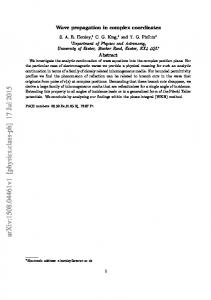
Figure 5: Asymptotic behavior: (Top) Wave Propagation, (Bottom) Deep Propagation.
25% of complex 1 constraints and 12% of complex 2 constraints. For this particular experiment we have used random constraint graphs because it is difficult to find a collection of benchmarks containing files with a gradually increasing number of constraints. Notice that these graphs are different from the constraint graphs that we would obtain from actual programs. The existence of edges in the constraint graphs of actual programs does not follow a normal distribution; instead, we observe that some special nodes tend do span or collect many edges. Furthermore, real constraint graphs tend to be more dense than our random graphs. For instance, after components had been collapsed using the deep propagation method, the random constraint graphs contain, on average, 0.87 edges per node. In comparison, the graphs produced in the same way for our real benchmarks range in density from 0.78 edges per nodes (sendmail) to 139.581 edges per node (wine). Another difference is the average size of the points-to set produced by the random graphs, which tend to be 5-10 times bigger than the average sizes observed in actual programs. Nevertheless, the random constraints give us an idea about the asymptotic behavior of each solver. The results obtained from running the algorithms on the MacOS environment are displayed in Figures 5 and 6. Each
Table 1: The Set of Benchmarks used in our experiments. Benchmark ex 300.twolf 197.parser 255.vortex sendmail 254.gap emacs 253.perl vim nethack 176.gcc ghostscript insight gdb gimp wine linux
Code ex tw pr vt sm gp em pl vm nh gc gs in gd gm wn lx
#Variables 3419 4,697 5,055 8,262 11,408 19,336 14,386 19,895 31,630 32,968 39,560 76,717 58,763 84,499 81,915 150,828 145,293
#Constraints 3,933 4,849 6,491 8,746 11,828 25,005 27,122 28,525 36,997 38,469 56,791 101,442 99,245 105,087 125,203 199,465 231,290
figure shows the line produced by fitting a polynomial of degree three on the data points. In order to measure the stability of each algorithm, we computed the variance of each point in relation to the regression curve. We observe that, for these constraint graphs, the Wave Propagation approach is the most stable, with an average variance of 4.31 seconds per constraint graph. The variance found for the other algorithms, in increasing order, is 8.819 for Heintze-Tardieu, 12.33 for Deep Propagation, 20.28 for Lazy Cycle Detection and 39.19 for the Pearce-Kelly-Hankin algorithm.
5.2
Running Time
In order to measure how the proposed algorithms perform in constraint graphs extracted from actual programs, we have used the benchmarks presented in [5], plus 12 benchmarks kindly provided to us by Ben Hardekopf, which include the six biggest integer programs in SPEC 2000. Table 1 shows the benchmarks. The constraints in these benchmarks are field-insensitive, that is, different variables in the same struct are treated as the same name. All the algorithms used in our tests are tuned to perform well with fieldinsensitive input constraints. The benchmarks have been preprocessed with an off-line variable substitution analysis [14]. The number of constraints includes all the constraint types - base, simple and complex - found in the programs after off-line variable substitution. Figure 7 compares the running time of the five algorithms in the Intel/MacOS setting. All the results are normalized to the Heintze-Tardieu (HT) algorithm. We observe that across the benchmarks, the Deep Propagation technique had the lowest geometric-mean, 0.82 of HT. The Wave Propagation method had the second lowest geometric-mean: 0.90 of HT. The average for the other algorithms are 1.77 for LCD, and 3.19 for PKH. The Deep Propagation method has the best overall performance; however, the Lazy Cycle Detection and the Wave Propagation techniques tend to outperform Deep Propagation for bigger benchmarks. For the three biggest
Table 2: The execution time of each algorithm (sec) on the Intel/MacOS setting.
ex tw pr vt sm gp em pl vm nh gc gs in gd gm wn lx Tot
WP 0.010 0.023 0.056 0.034 0.106 0.316 0.997 0.895 1.810 0.167 0.813 51.50 67.47 32.74 33.36 1,327.3 560.0 2,055.1
DP 0.004 0.011 0.028 0.024 0.107 0.293 0.793 0.853 1.673 0.111 0.619 138.07 45.05 62.86 53.92 1,423.5 349.7 2,099.5
HT 0.005 0.015 0.041 0.023 0.114 0.336 1.445 1.402 2.150 0.154 0.742 219.15 42.54 72.32 63.21 1,578.3 382.4 2,364.8
LCD 0.012 0.075 0.097 0.070 0.229 0.725 2.756 3.589 4.442 0.362 3.397 175.81 62.68 87.11 38.13 983.6 281.1 1,644.8
PKH 0.041 0.078 0.315 0.120 0.422 1.480 2.408 4.551 12.25 0.559 2.910 173.91 122.06 164.87 101.65 1987.5 1,126.2 3,701.3
benchmarks, gimp, wine and linux, we have the following geometric means: DP = 0.87, WP = 0.89, LCD = 0.65 and PKH = 1.81. Figure 8 compares the five algorithm in the AMD/Linux execution environment. We have observed small changes on the relative execution times for some of the benchmarks. In particular, Wave Propagation outperforms Lazy Cycle Detection for Wine, the most time consuming benchmark. Also the Heintze-Tardieu algorithm has the second best geometricmean. However, the overall time pattern remains the same: the Deep Propagation method presents the best geometricmean: 0.89 of HT. The other means are WP = 1.04, LCD = 1.65 and PKH = 3.09. Considering only the three biggest benchmarks, we have: WP = 0.83, DP = 1.0, LCD = 0.69 and PKH = 1.97. Table 2 gives the absolute running time of all the algorithms in the Intex/MacOS environment, and Table 3 gives the equivalent numbers for the AMD/Linux setting. Overall, the MacOS environment accounted for the fastest times. The total running time, in seconds, of all the algorithms in the MacOS Setting is LCD = 1,656.99, WP = 2,094.13, DP = 2,086.52, HT = 2,376.07 and PKH = 3,733.37. Notice that, although LCD has a lower geometric mean than DP or WP, its absolute running time in this environment is better, because it produces the fastest results for Wine and the Linux kernel, the biggest benchmarks. On the other hand, the absolute running times in the AMD/Linux platform show the wave propagation with the best times: WP = 2,783.22, LCD = 2,817.8, HT = 3,709.01, DP = 3,916.68 and PKH = 6,565.51. We speculate that the relative variation between WP and LCD is due to the amount of free memory in the different machines, which explains the memoryhungry WP outperforming LCD on the machine with larger RAM.
200
0
150 0
100
50
100
400 300 200
Time (seconds)
Time (seconds)
500
600
200 150 100
Time (seconds)
50 0 0
20
40
60
80
100
120
0
Number of Constraints (x 104)
20
40
60
80
100
0
120
Number of Constraints (x 104)
20
40
60
80
100
120
Number of Constraints (x 104)
Figure 6: Asymptotic behavior: (Left) Heintze-Tardieu, (Middle) Pearce-Kelly-Hankin (Right) Lazy Cycle Detection.
WP
DP
LCD
PKH
10
1
0.1
ex
tw
pr
vt
sm
gp
em
pl
vm
nh
gc
gs
in
gd
gm
wn
lx GeoM
Figure 7: Running time comparison between the five solvers (Intel running MacOSX 10.4.1).
We close this section pointing how the time is divided among the three phases of the wave propagation method. Notice that, although the edge insertion phase and the wave propagation phase have the same complexity, the latter is much faster in actual applications. The chart in Figure 9 shows how the time is divided between the three main phases of this algorithm. As it can be noted, the insertion of new edges in the constraint graph accounts for over 89% of the total running time of the algorithm for the biggest benchmarks. This difference happens because the search for cycles is linear on the number of edges of the constraint graph, and because the wave propagation phase only propagates differences between points-to sets.
5.3
Add Edges
Wave Propagation
Collapse Cycles
1.0
0.5
0
ex tw pr vt sm gp em pl vm nh gc gs in gd gm wn lx
Memory Usage
Figure 10 shows the memory consumption among the five tested algorithms. HT is the most economical across the benchmark suite, with the lowest geometric-mean. The next algorithm, DP, uses 1% more memory on average than HT. The memory usage for the other algorithm, relative to HT, is LCD = 1.07, PKH = 1.16 and WP = 1.42. The wave propagation method demands more memory because it stores an extra bitset per each variable - the last points-to set prop-
Figure 9: Time division in the wave propagation method in the Intel/MacOS setting.
agated for that variable, plus an extra bitset per complex constraint - the last points-to set used to add edges to the
WP
DP
LCD
PKH
10
1
0.1
ex
tw
pr
vt
sm
gp
em
pl
vm
nh
gc
gs
in
gd
gm
wn
lx GeoM
Figure 8: Running time comparison between the five solvers (AMD Opteron running Linux Ubuntu 6.06.2).
Table 4: Summary of Experiments
Table 3: The execution time of each algorithm (sec) on the AMD/Linux setting.
ex tw pr vt sm gp em pl vm nh gc gs in gd gm wn lx Tot
WP 0.021 0.022 0.064 0.044 0.148 0.642 2.407 1.262 3.399 0.277 1.081 90.14 131.45 67.38 64.69 1,191.4 1,227.9 2,783.2
DP 0.009 0.011 0.032 0.029 0.213 0.397 1.300 1.326 2.757 0.189 0.880 244.20 88.24 103.77 98.24 2,769.5 605.7 3,916.7
HT 0.020 0.016 0.046 0.028 0.151 0.434 2.098 1.924 3.926 0.213 0.985 346.24 62.75 106.10 102.21 2,396.7 666.61 3,709.0
LCD 0.025 0.061 0.084 0.071 0.269 0.867 4.094 4.818 6.161 0.441 3.886 277.08 90.12 123.05 60.38 1,754.3 501.69 2,817.8
PKH 0.103 0.079 0.338 0.131 0.514 2.064 3.357 6.683 21.971 0.643 3.84 301.68 190.42 283.42 173.65 4,013.4 1,784.2 6,565.5
constraint graph. Wine is responsible for the largest memory consumption among all the algorithms. The amount of memory that each algorithm needs to process this benchmark is: DP = 1,561M, LCD = 1,750M, PKH = 1,778M, HT = 2,095M and WP = 2,421M. Because the numbers for Wine dominate all the other benchmarks, although HT had the lowest geometric mean, in absolute terms DP was the most economical algorithm. If we sum up the memory required by each algorithm to process all the benchmarks, we get: DP = 3,954M, LCD = 4,121M, PKH = 4,255M, HT = 4,328M and WP = 5,881M.
5.4
Summary of Experiments
GT OSX GT LX AT OSX AT LX GM AM Variance
DP 0.82 (*) 0.89 (*) 2,099 3,917 1.01 3,954 (*) 12.33
WP 0.90 1.04 2,055 2,783 (*) 1.42 5,881 4.31 (*)
LCD 1.77 1.65 1,645 (*) 2,818 1.07 4,121 20.28
HT 1.0 1.0 2,364 3,709 1.0 (*) 4,328 8.82
PKH 3.19 1.97 3,701 6,566 1.16 4,255 39.19
Table 4 summarizes all the results described in this Section. GT stands for geometric mean of running time, AT stands for absolute running time, OSX stands for MacOS/Intel, LX stands for linux/AMD, GM stands for geometric mean of memory consumption and AM stands for absolute memory consumption.
6.
CONCLUSION AND FUTURE WORK
This paper has presented two new algorithms for solving Andersen based points-to analysis: the Wave Propagation and the Deep Propagation methods. As discussed in Section 5, these algorithms improve the current state of the art in many different directions. One of the main motivations for the Wave Propagation method is to be a base algorithm for parallelizing Andersen style points-to analyses, and we are currently working on such an implementation. Cycle elimination complicates the parallelization of points-to solvers, because this optimization may force the locking of a potentially linear number of nodes in the constraint graph, in order to avoid data races. The wave propagation algorithm is an attempt to get around this problem, because the detection of cycles is separate from the propagation of points-to sets. The detection of strongly connected components, the first phase of the new algorithm, has a well-known parallel implementation [4]. Once connected components are discovered, each of them can be collapsed by a different thread. As observed in Figure 9, the insertion of edges accounts for most of the execution time of the Wave Propagation method.
3
WP
DP
LCD
PKH
2
1
0
ex
tw
pr
vt
sm
gp
em
pl
vm
nh
gc
gs
in
gd
gm
wn
lx GeoM
Figure 10: Memory usage in AMD Opteron running Linux Ubuntu 6.06.2.
Although this phase is not an embarrassingly parallel task, its parallelization requires the locking of a constant number of nodes per thread. When processing a constraint such as l ⊇ ∗r, a thread must lock the old and current points-to set of node r. During the insertion of an edge (v, l), where v ∈ Pcur (r), the edge set of node v must be locked. When updating the current points-to set of node l, Pcur (l) and Pold (v) must be locked. Another future direction is to verify how much the Hybrid Cycle Detection algorithm proposed in [5] improves the Deep Propagation and the Wave Propagation methods. We would like to verify also how different constraint orderings impact the Deep Propagation method. Algorithm 6 first processes all the complex 1 constraints and then all the complex 2 constraints, but it is possible that different orderings improve its running time, as some preliminary experiments have shown. acknowledgment We thank Ben Hardekopft for generously providing the benchmarks used in our experiments and reviewing a draft of this paper.
7.
REFERENCES
[1] Lars Ole Andersen. Program Analysis and Specialization for the C Programming Language. PhD thesis, DIKU, University of Copenhagen, 1994. [2] Ben-Chung Cheng and Wen-Mei W. Hwu. Modular interprocedural pointer analysis using access paths: design, implementation, and evaluation. In PLDI, pages 57–69, 2000. [3] Manuel Fahndrich, Jeffrey S. Foster, Zhendong Su, and Alexander Aiken. Partial online cycle elimination in inclusion constraint graphs. In PLDI, pages 85–96, 1998. [4] Alan Gibbons. Efficient Parallel Algorithms. Cambridge University Press, 1988. [5] Ben Hardekopf and Calvin Lin. The ant and the grasshopper: fast and accurate pointer analysis for millions of lines of code. In PLDI, pages 290–299, 2007. [6] Ben Hardekopf and Calvin Lin. Exploiting pointer and location equivalence to optimize pointer analysis. In
SAS, pages 265–280, 2007. [7] Nevin Heintze and Olivier Tardieu. Ultra-fast aliasing analysis using CLA: A million lines of C code in a second. In PLDI, pages 254–263, 2001. [8] Susan Horwitz. Precise flow-insensitive may-alias analysis is NP-hard. ACM Trans. Program. Lang. Syst., 19(1):1–6, 1997. [9] Robert Kennedy, Sun Chan, Shin-Ming Liu, Raymond Lo, Peng Tu, and Fred C. Chow. Partial redundancy elimination in SSA form. ACM Trans. Program. Lang. Syst., 21(3):627–676, 1999. [10] Chris Lattner and Vikram S. Adve. Llvm: A compilation framework for lifelong program analysis & transformation. In CGO, pages 75–88, 2004. [11] Esko Nuutila and Eljas Soisalon-Soininen. On finding the strongly connected components in a directed graph. Inf. Process. Lett., 49(1):9–14, 1994. [12] David J. Pearce, Paul H. J. Kelly, and Chris Hankin. Online cycle detection and difference propagation for pointer analysis. In SCAM, pages 3–12, 2003. [13] David J. Pearce, Paul H. J. Kelly, and Chris Hankin. Efficient field-sensitive pointer analysis for C. In PASTE, pages 37–42, 2004. [14] Atanas Rountev and Satish Chandra. Off-line variable substitution for scaling points-to analysis. In PLDI, pages 47–56, 2000. [15] Bjarne Steensgaard. Points-to analysis in almost linear time. In POPL, pages 32–41, 1996. [16] Robert Endre Tarjan. Depth-first search and linear graph algorithms. SIAM J. Comput., 1(2):146–160, 1972. [17] John Whaley and Monica S. Lam. Cloning-based context-sensitive pointer alias analysis using binary decision diagrams. In PLDI, pages 131–144, 2004. [18] Jianwen Zhu. Towards scalable flow and context sensitive pointer analysis. In DAC, pages 831–836, 2005.