Wavelet Modulation Performance in Fading Conditions Marius Oltean1 Abstract – This paper proposes an investigation of wavelet based multi-carrier modulation performance in flat fading radio channels. Transmission BER is computed and analyzed against the classical Orthogonal Frequency Division Multiplexing (OFDM) performance in various scenarios with respect to the Doppler shift influence and to the noise level. Keywords: OFDM, wavelet-based OFDM, fading, Doppler shift.
I. INTRODUCTION Multi-carrier modulation techniques are widely used in the last decade in various transmission standards in wired and wireless channels. Amongst others, versions of Fourier-based OFDM are employed at the physical level to provide good performance over the air interface in systems like Digital Audio & Video Broadcasting (DAVB), WiMAX (described by IEEE 802.16) or WiFi (802.11). This proves the reliability and the efficiency of the multi-carrier modulation concept, which is very well suited to radio transmissions. Besides its incontestable advantages, OFDM presents some well known drawbacks as diminished spectral efficiency because of the cyclic prefix (CP) overhead, slow decay of the out-of-band side-lobes, high sensitivity to time and frequency synchronization, increased peak-to-average-power ratio [1,2]. Recent research focused on the multi-carrier transmission techniques [3,4], highlighted that some of these disadvantages can be steadily counteracted using wavelet carriers instead of OFDM's complex exponential waveforms. Due to the fact that these wavelet carriers form an orthogonal family over the duration of a transmitted symbol, they can be separated at receiver's side by correlation techniques. The authors in [5] have shown that wavelet-based OFDM (WOFDM) has better spectral efficiency, is simpler and at least as rapid as OFDM in practical implementations. Furthermore, the performance of the two systems is similar in AWGN channels. Note however that, from this point of view, the real gain of multi-carrier techniques can be highlighted in conditions specific to the radio channels, which are both frequency-selective and time-variant. With respect to these conditions, the author will investigate the OFDM and WOFDM performance in different flat fading scenarios. A deeper analysis of the wavelet based method is performed, taking into account the influence of the wavelet's mother, as well as of the
number of decomposition levels used in Inverse Discrete Wavelet Transform (IDWT) computation. In the next section, an overview of the multicarrier modulation concept is provided, focusing on the WOFDM principles. The third section will illustrate the simulation scenarios, whose results will be shown and commented in section 4. The last section is dedicated to concluding remarks and to some possible future directions for the continuation of the present work. II. MULTI-CARRIER TRANSMISSIONS AND WAVELETS Largely used in the modern communication systems, Orthogonal Frequency Division Multiplexing (OFDM) relies on a multicarrier approach, where data is transmitted using several parallel substreams. Every stream modulates a different complex exponential subcarrier, the used subcarriers being orthogonal to each other. The orthogonality is the key point that allows subcarrier separation at receiver. The multicarrier approach has the advantage of a long symbol duration, provided by the simultaneous transmission of several low-rate parallel streams. OFDM implementation is based on the Fast Fourier Transform (FFT) algorithm, which allows reduced complexity and low implementation cost. The idea which connects OFDM and wavelets is that in the same manner that the complex exponentials define an orthonormal basis for any periodic signal, a wavelet family forms a complete orthonormal basis for L2 (ℜ) : ⎧1, if j = m and k = n < ψ j, k ( t ), Ψm ,n ( t ) >= ⎨ 0, otherwise ⎩
(1)
Wavelet family members from (1) can be obtained by translating and scaling a unique function called wavelets mother and denoted by ψ ( t ) , according to (2): ψ j, k ( t ) = s 0− j / 2 ψ (s 0− j ⋅ t − kτ 0 )
(2)
Equation 2 corresponds to a sampled version of a wavelet family, the discrete variables being s0 (the scale) and k (the position within the scale). The relation above indicates that all the members of the wavelet family {Ψj, k ( t ) = 2 − j / 2 Ψ (2 − j t − k )}k∈Z
1 Facultatea de Electronică şi Telecomunicaţii, Departamentul Comunicaţii Bd. V. Pârvan Nr. 2, 300223 Timişoara, e-mail
[email protected]
(we considered s0=2 and τ0=1) are orthogonal to each other. Consequently, if instead of complex exponential waveforms we use wavelet carriers, we will still be able to separate these subcarriers at receiver, due to their orthogonality. This is the main idea, which lies behind the wavelet-based OFDM techniques [3,6]. As for the classical OFDM, the WOFDM symbol can be generated by digital signal processing techniques, such as IDWT. In this case, the transmitted signal is synthesized from the wavelet coefficients w j, k =< s( t ), ψ j, k ( t ) > located at the k-th position from scale j (j=1,…, J) and from the approximation coefficients a J , k =< s( t ), ϕJ , k ( t ) > ,
located at the k-th position from the coarsest scale J: J
∞
∞
s( t ) = ∑ ∑ w j, k ψ j.k ( t ) + ∑ a J , k ϕ J , k ( t ) k = −∞
Note that, in practice, a sampled version of the signal s(t) is generated by means of Malat’s Fast Wavelet Transform (FWT) algorithm [7]. In this case, the data vector at IDWT input is composed as follows: data = [{a J ,k },{w J ,k },{w J −1,k },...,{w 1,k }]
(4)
This data sequence is modulated onto a contiguous finite set of dyadic frequency bands and onto a finite number of time positions k within each scale. The practical implementation of such a system requires finite-length dyadic data sequences at system input. If we denote by N the length of our input data sequence (which must be a power of 2), then the maximum number of decomposition levels for the DWT equals L=log2(N), and equation (3) becomes: J 2 L− j
2 L−J
j =1 k =1
k =1
s( t ) = ∑ ∑ w j, k ψ j.k ( t ) + ∑ a J , k ϕ J , k ( t )
(5)
where J stands for the number of decomposition levels used, (whose the maximum value is L). III. SIMULATION SCENARIO The BER performance of WOFDM and OFDM will be compared in AWGN and flat fading Rayleigh channel. The transmission chain used for simulations is shown in figure 1. ray[n] [w] [west]
IDWT/ IFFT Decision
p[n]
s[n] DWT/ FFT
r[n]
Fig.1: Baseband implementation of a WOFDM system.
For the case of a classical OFDM system, the input data vector [w] can be interpreted as being composed of frequency-domain coefficients. These coefficients are randomly generated from bipolar symbols +1 and -1, such a way that the output of IFFT block to generate a real sequence [5]. If a WOFDM transmission is implemented instead, then the input data vector [w] represents a sequence of wavelet-domain detail and approximation coefficients. The composition of the time-domain signal (the "WOFDM symbol") is detailed in figure 2, with respect to equation 5. Input data {aJ} {wJ} {wJ-1}
IDWT
j =1k = −∞
(3)
A. The transmitter
s[n]
{w1} Fig. 2: Composition of WOFDM symbol using IDWT: practical implementation.
Note that in figure above, J represents the coarsest scale used for IDWT computation. The choice of the approximation and detail coefficients which compose the input data vector (see fig. 2) can be done in different manners. The authors in [8] consider the data at scale J-1 as being a repetition of the useful stream from the previous coarser scale J. Since at scale J-1 we have two times more wavelet coefficients, one can state that at this scale we transmit the same data as at scale J but with a two times higher rate. The author's approach in this paper is to transmit independent data streams at each scale. This data corresponds to a vector of N equally likely bipolar symbols ±1. The meaning of each symbol composing the vector is given by equation 4: first we have the approximation coefficients, then the coarsest scale wavelet coefficients, next finer scale wavelet coefficients etc. B. The channel
The radio channels exhibit small scale fading, which confer to this transmission environment two independent characteristics: time variance and frequency selectivity [9]. The variance in time of the radio channel's behavior can be expressed by the mean of the Doppler shift parameter, which depends on the relative motion between transmitter and receiver (assuming mobile communications) and on the carrier frequency used for transmission. The author uses in this paper a normalized version of this parameter: f m = f d ⋅ TS
(6)
where TS is the duration of a transmission symbol (from the data vector shown in fig.2) . The values taken into account for fm in our simulations belong to the set {0.001, 0.005, 0.01, 0.05}. In slow fading scenarios, TS must be much smaller than the coherence time of the channel expressed as: 0.423 TC = fd
pdf ( x σ) =
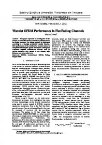
IV. RESULTS AND DISCUSSIONS Simulations were made under Matlab 7. For both investigated methods, the author considers the transmission of 10000 data blocks of 1024 symbols each. For the OFDM simulations, 512 complex symbols were composed from 1024 randomly generated bipolar values (+ 1 and -1), in order to obtain real values at the output of IFFT block. Neither synchronization, nor equalization issues were taken into account. The first set of simulations aims to investigate the performance of the two methods in AWGN channels. For the WOFDM system, there is a matter of choice what will be the wavelets mother used in DWT computation and what will be the number of iterations, according to Mallat’s algorithm. In the following simulations, the author investigates what is the influence of these choices on the overall system performance. As indicated by figure 3, both systems perform identically in white noise conditions. Furthermore, the computed BER is similar to BPSK case.
(7)
−x 2
10
10
10
10
10
10
2σ 2
σ2
(8)
In our simulations we consider unitary variance (σ2=1). This is a simplifying hypothesis, because the variance of the signal obtained after multiplication (see equation 9) is equal to the variance of the useful signal, s. A white noise p[n] is then added to the signal above, obtaining the sequence r[n] to be processed by the demodulator: r[n ] = s[n ] ⋅ ray[n ] + p[n ]
(9)
C. The receiver
The receiver is composed of a demodulator (the FFT or DWT block respectively) and a simple detector using a threshold comparison. Neither synchronization, nor equalization issues are taken into
-1
-2
-3
BER
Taking into account the two formulas (6,7), our worst case scenario (fm=0.05) leads to a coherence time TC which is approximately 8 times higher than TS. In the best case (the lowest Doppler shift), the coherence time is 400 times longer than the symbol duration. These values seem to fit to the slow fading model, where the channel stays unchanged for the duration of a symbol. Though, when evaluating the channel behavior, one should take into account that in multi-carrier communications the transmitted symbol is longer. Usually, since the whole data vector is required at demodulator to identify the transmitted symbols, we can consider that the multicarrier symbol duration (an OFDM or a WOFDM block) is N times longer than the serial symbols brought at system's input. Note that in these conditions, the channel response changes during the transmission of one symbol, or block. From the frequency selectivity point of view, the scenario taken into account refers to flat fading model, where the frequency response of the channel is considered approximately constant in the transmission band. This means reduced frequency selectivity and reduced time dispersion of the signal. Small scale fading can be modeled as a Rayleigh distribution, generated using the method described in [10]. The impact of the Rayleigh flat fading is given by the multiplicative ray[n]. Rayleigh pdf is described in equation 8: x ⋅e
consideration. The performance is measured using the BER, computed for every simulation scenario described above.
-4
:real FOFDM :Haar W OFDM -1 level :Haar W OFDM -4 levels Daubechies 10 W OFDM -1 level Daubechies 10 W OFDM -4 levels BPSK -Theoretical curve
-5
-6
0
1
2
3
4
5 SNR [dB]
6
7
8
9
10
Fig.3: BER performance of FOFDM and WOFDM with different wavelet mothers in AWGN conditions.
As an additional conclusion, figure 3 clearly shows that in such channels, BER performance doesn't depend neither on the type of wavelets mother, nor on the number of decomposition levels used in DWT computation. All the following simulated scenarios refer to flat Rayleigh fading channels. Two different wavelet mothers were used for DWT computations: Haar and Daubechies-10. Thus, the channel exhibit flatness (no frequency selectivity) and a variant behavior over the time. In this context, OFDM and WOFDM are first analyzed independentely against Doppler shift parameter. The results shown in figure 4 meet the expectations, in the sense that both systems exhibit a performance degradation for increased Doppler shift value.
0
10
displacement of one carrier will move its position and will transform this carrier into an interfering source for the other ones. Furthermore, for an OFDM system, the following remark can be made: higher the number of subcarriers, lower their frequency separation and higher the probability of interference. Next, the author investigates the effect of wavelets mother used for IDWT computation on the BER performance of a WOFDM system. Simulations were made for two different wavelets: Haar and Daubechies-10. The results are shown in figure 6 (a and b).
-1
-2
10
:OFDM,fm=0.001 :OFDM,fm=0.005 :OFDM,fm=0.01 :OFDM,fm=0.05 :Haar WOFDM, fm=0.001,4 levels :Haar WOFDM, fm=0.005, 4 levels :Haar WOFDM, fm=0.01, 4 levels :Haar WOFDM, fm=0.05, 4 levels
-3
10
-4
10
0
2
4
6
8
10 12 SNR [dB]
14
16
18
0
20
10
: : : :
Fig.4: BER performance in various Doppler shift scenarios.
Daub10 WOFDM,fm=0.001,1 level Daub10 WOFDM,fm=0.05,1 level Haar WOFDM,fm=0.001,1 level Haar WOFDM,fm=0.05,1 level
-1
0
10
: : : :
OFDM,fm=0.01 OFDM,fm=0.05 Daub10 WOFDM,fm=0.01,1 level Daub10 WOFDM,fm=0.05,1 level
-1
10
-2
10
-3
10
0
2
4
6
8
10 12 SNR [dB]
14
16
18
20
Fig.5: BER performance of OFDM/WOFDM at high Doppler shift values.
Carefully examining this figure, one can notice an excellent gain of WOFDM (approximately 10 dB at the highest Doppler taken into account). These results can be explained by the well known sensitivity of OFDM to the time variant character of the radio channel. Indeed, the orthogonality of the sine carriers in OFDM is very fragile: a small Doppler
10
BER
Even if the Doppler shift-induced degradation has the same range (three times more errors for fm=0.05 compared to fm=0.001) for the two methods, some differences between WOFDM and OFDM can be highlighted when we analyze fig. 4 into a more detailed fashion. First, WOFDM works better: at a SNR of 20dB, the worst case when using wavelets performs better than the best case (the lowest Doppler) in the classical OFDM. Second, WOFDM is generally less sensitive to Doppler, since this system barely shows a 2 dB loss when moving from fm=0.001 to a then times higher value. For the classical OFDM, the loss is of almost 10 dB for a BER fixed at 2%. Third, the negative impact of Doppler shift can be clearly highlighted only at high SNR values (above 10 dB), because at low SNR the main amount of errors is brought by the noise. These results are strengthened by figure 5, where WOFDM is simulated with a different wavelets mother (Daubechies-10).
BER
BER
10
-2
10
-3
10
0
2
4
6
8
10 12 SNR [dB]
14
16
18
20
Fig.6a: The influence of the wavelets mother choice in a WOFDM system:1 decomposition level.
Several conclusions can be drawn after studying figure 6a. At low Doppler, no significant difference exists between the two wavelets. If the value of this parameter is increased, one can notice an important gain brought by the Haar’s wavelet (about 4dB). This gain may rely on the poor frequency (and good time) localization of this wavelet, when compared to Daubechies-10. Thus, the variability in time of the radio channel seems to cause more problems when carrier waves with good frequency localization are used (this conclusion could also refer to OFDM’s sine carriers, as an extreme case). Note yet that this conclusion should be enforced by well structured theoretical computations and by more extensive simulations, including several types of wavelets. Figure 6b strengthens the previous remarks for a different number of decomposition levels. However, the results are slightly different and a significant difference can be highlighted even at low Doppler shifts. Thus, the gain in the case of Haar based WOFDM ranges between 3dB for fm=0.001 and 5dB for fm=0.05. This promising result can be explained by the fact that Haar's wavelet has the best time localization amongst all wavelet's mother, and, implicitly, it spans over a wide range of frequencies. Another argument , which remains only at a stage of intuitive remark, is that Haar's wavelet matches "the best" to the bipolar data transmission (a wavelet's mother looks like a sequence of two symbols -1 and +1 transmitted sequentially).
0
10
0
10
: : : :
-1
-1
-2
10
Haar WOFDM,fm=0.001,4 levels Haar WOFDM,fm=0.05,4 levels Haar WOFDM,fm=0.001,1 level Haar WOFDM,fm=0.05,1 level
-2
10
-3
-3
10
10
-4
10
: : : :
10
BER
BER
10
Daub10 WOFDM,fm=0.001,4 levels Daub10 WOFDM,fm=0.05,4 levels Haar WOFDM,fm=0.001,4 levels Haar WOFDM,fm=0.05,4 levels
-4
0
2
4
6
8
10 12 SNR [dB]
14
16
18
20
Fig.6b: The influence of the wavelets mother choice in a WOFDM system:4 decomposition levels.
The last goal of this paper is to analyze what is the impact of the number of decomposition levels used for DWT/IDWT computation, on the overall system’s performance. Simulations were made for the two wavelets mother above, with one and four iterations respectively. The results are displayed in figure 7 (a and b). 0
10
: : : :
Daub10 WOFDM,fm=0.001,4 levels Daub10 WOFDM,fm=0.05,4 levels Daub10 WOFDM,fm=0.001,1 level Daub10 WOFDM,fm=0.05,1 level
-1
BER
10
10
0
2
4
6
8
10 12 SNR [dB]
14
16
18
20
Fig.7b: The influence of the number of iterations used for DWT/IDWT computation: Haar wavelets mother.
2, the data at the IDWT synthesizer input will be composed of aJ and wJ only. If we refer to equation 3, then wJ coefficients will modulate a wavelet Ψ1(t)= Ψ(t/2). When more iterations are used (4 iterations in our simulations), then the wavelet carriers will be not only those from the finest scale but wavelets from coarser scales too (Ψ2(t)= Ψ1(t/4), Ψ3(t)= Ψ1(t/8) etc). Previous studies made [6, 8] have shown that higher Doppler shifts (short coherence time) will mainly affect the symbols transmitted at coarser scales, where symbol (or equivalently "sample") duration is longer, becoming comparable with channel's coherence time. This can be highlighted only by carrying out the evaluation of errors distribution "per scale", which will be the subject of a future paper.
-2
10
V. CONCLUSIONS AND FURTHER WORK -3
10
0
2
4
6
8
10 12 SNR [dB]
14
16
18
20
Fig.7a: The influence of the number of iterations used for DWT/IDWT computation: Daubechies-10 wavelets mother.
Figure 7a supports the following hypothesis: higher the number of iterations used in DWT/IDWT computation, lower the system protection against Doppler shift and poorer the system performance. The degradation brought by an increased number of iterations ranges from 2 to 5 dB. On the other hand, the same conclusion can be drawn from figure 7b. However, Haar wavelets mother exhibits less sensitivity to the number of decomposition levels: no significant difference at low Doppler (fm=0.001) and about 4 dB gain when a single iteration is used at fm=0.05. These observations are interesting and their interpretation is not straightforward. One possible explanation is given in the following. When a single iteration is used for IDWT computation, the wavelet carrier employed has the best time localization and the poorest frequency localization amongst all other wavelets from the same family. With respect to figure
The performance of wavelet-based OFDM in flat Rayleigh fading conditions is investigated in this paper. The author carries out a comparison between this technique and the classical OFDM, based on complex exponential carriers. It is proven by simulation means that, while exhibiting similar behavior in AWGN channels, the two techniques perform different in flat Rayleigh fading conditions. Showing less sensitivity to the Doppler shift caused by the time-variant character of the radio channel, WOFDM has better BER performance, mainly at high Doppler shift values (a gain of more than 10 dB under certain circumstances). A second goal of this paper was to study what is the influence of certain parameters used for WOFDM implementation: the wavelets mother and the number of decomposition levels used in DWT/IDWT computation. Thus, Haar-based WOFDM works better than Daubechies 10 –based WOFDM. Intuitively, this can be explained by the poor frequency localization of the first studied wavelet, which is less affected by the frequency offset caused by the Doppler effect. On the other hand, the number of iterations used for DWT/IDWT computation proves to be important too. Noticeable differences
were observed especially in the case of Daubechies10 wavelet, which performs significantly better when a single iteration (a single decomposition level is used). The explanation resides in the inherent structure of WOFDM, which acts “across the scales”: less iterations means finer scales, shorter duration wavelet carriers (and implicitly shorter transmitted samples). Next, shorter the data symbols on a scale means less sensitivity to the Doppler shift (the coherence time of the channel being significantly higher than the symbol time). These interesting conclusions open the road towards some new research directions on this subject. Thus, the real effect of wavelet's mother choice can be clearly identified only be a more comprehensive theoretical and practical study, which should be carried out on more wavelets families (e.g. Symmlet, Coiflet, Daubechies etc). On the other hand, the importance of the number of decomposition levels can be investigated in a more detailed fashion only by computing "number of errors per scale" statistics. Intuitively, these "BER across scales" statistics could be used in order to select the appropriated error correcting codes which would lead to an optimized performance. Finally, the next logical step in this direction will be to take into consideration the second crucial characteristic of the radio channel, besides its timevariant behavior, namely its frequency selectivity. Indeed, the influence of all parameters considered in this study could be redefined in a frequency-selective context, where equalizations issues become critical.
REFERENCES [1] M. Huemer, A. Koppler, L. Reindl, R. Weigel, “A Review of Cyclically Extended Single Carrier Transmission with Frequency Domain Equalization for Broadband Wireless Transmission”, European Transactions on Communications (ETT), Vol. 14, No. 4, pp. 329-341, July/August 2003. [2] M. Oltean, “An Introduction to Orthogonal Frequency Division Multiplexing”, Analele Universitatii Oradea, 2004, Fascicola Electrotehnica, Sectiunea Electronica,pp.180-185. [3] F. Zhao, H. Zhang, D. Yuan, "Performance of COFDM with Different orthogonal Basis on AWGN and frequency Selective Channel ", in Proc. of IEEE International Symposium on Emerging Technologies: Mobile and Wireless Communications, Shanghai, China, May 31 – June 2, 2004, pp. 473-475. [4]Rainmaker Technologies Inc., "RM Wavelet Based PHY Proposal for 802.16.3", available on-line at: http://www.ieee802.org/16/tg3/contrib/802163c-01_12.pdf [5] M. Oltean, M. Nafornita, "Efficient Pulse Shaping and Robust Data Transmission Using Wavelets", accepted to the third IEEE International Symposium on Intelligent Signal Processing, WISP 2007, Alcala de Henares, Spain. [6] A. E. Bell and M.J. Manglani, "Wavelet Modulation in Rayleigh Fading Channels: Improved Performance and Channel Identification", Proceedings of IEEE International Conference on Acoustics, Speech and Signal Processing ICASSP 2002, pp. 28132816, Orlando-Florida, May 2002. [7] S. Mallat, A wavelet tour of signal processing (second edition), Academic Press,1999. [8] M. J. Manglani and A. E. Bell, "Wavelet Modulation Performance in Gaussian and Rayleigh Fading Channels" Proceedings of MILCOM 2001, McLean, VA, October 2001. [9] B. Sklar, “Rayleigh Fading Channels in Mobile Digital Communication Systems- Part I: Characterization”, IEEE Commun. Mag., July 1997. [10] K. E. Baddour, N. C. Beaulieu, “Autoregressive modeling for fading channel simulation”, IEEE Trans. Wireless Communications, pp.1650-1662, July 2005.