Weakly Connected Oscillatory Networks for Pattern ... - CiteSeerX

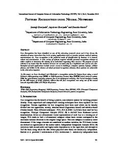
Weakly Connected Oscillatory Networks for Pattern Recognition via Associative and Dynamic Memories Fernando Corinto, Michele Bonnin, and Marco Gilli Department of Electronics, Politecnico di Torino, Italy. Abstract Many studies in neuroscience have shown that nonlinear oscillatory networks represent a bioinspired models for information and image processing. Recent studies on the thalamo-cortical system have shown that weakly connected oscillatory networks (WCONs) exhibit associative properties and can be exploited for dynamic pattern recognition. In this manuscript we focus on WCONs, composed of oscillators that admit of a Lur’e like description and are organized in such a way that they communicate one another, through a common medium. The main dynamic features are investigated by exploiting the phase deviation equation (i.e. the equation that describes the phase deviation due to the weak coupling). Firstly a very accurate analytic expression of the phase deviation equation is derived, via the joint application of the describing function technique and of Malkin’s Theorem. Furthermore, by using a simple learning algorithm, the phase-deviation equation is designed in such a way that given sets of patterns can be stored and recalled. In particular, two models of WCONs are given as examples of associative and dynamic memories.

1

Introduction

Historically, the mechanisms of synaptic adaptation and the neuronal unit models are the subjects of many theoretical works in the neuroscience. It is widely accepted that natural and artificial biological systems can be accurately mimicked by neural networks in which the neurons, modeled as the McCulloch-Pitts neuronal units [Hopfield, 1982] or ”integrate and fire” cells [Kandel et al., 2000], are coupled via adaptive synapses. Experimental observations have shown that if the neuronal activity, given by the accumulation (integration) of the spikes coming from the other neurons via the synapses, is greater than a certain threshold then the neuron fires repetitive spikes, otherwise the neuron remains quiescent [Kandel et al., 2000]. A different approach for modeling neuronal activity is founded on the replacement of neurons with periodic oscillators, where the phase of the oscillator plays the role of the spike time [Kandel et al., 2000]. Oscillatory neuronal activity can be recognized in several biological systems, including central pattern generators, visual and olfactory systems, etc. Indeed, recent studies in neuroscience have shown that some significant features of the visual systems [Gray et al., 1989; Engel et al., 1992], like the binding problem [Roskies, 1999], can be investigated by exploiting nonlinear oscillatory network models [Schillen & K¨onig, 1994]. Some studies on the thalamo-cortical system have also suggested new architectures for neurocomputers, that consist of coupled arrays of oscillators, with a periodic and/or complex dynamic behavior (including the possibility of chaos) [Hoppensteadt & Izhikevich, 1997; Hoppensteadt & Izhikevich, 1999]. On the other hand, the paradigm of nonlinear oscillatory networks have been widely used not only in Biology, but also in Physics and Engineering for modeling complex space-time phenomena [Kuramoto, 1984]. The most significant and worth studying property of the oscillatory systems is the synchronization, either when they are coupled with other oscillators or when they are subject to an 1

external driving signal. The synchronized states, with nontrivial phase relations among the oscillators, depend on the coupling laws used for modeling the synapses. In particular, it has been shown that weak couplings allow oscillatory networks to operate as Hopfield neural networks, whose attractors are limit cycles instead of equilibrium points [Hoppensteadt & Izhikevich, 1997; Hoppensteadt & Izhikevich, 1999]. In this work we focus essentially on Weakly Connected Oscillatory Networks (WCONs) that represent bio-inspired architectures for information and image processing. From the mathematical point of view a weakly connected oscillatory network consists of a large system of coupled nonlinear ordinary differential equations (ODEs), that may exhibit a rich spatiotemporal dynamics, including several attractors and bifurcation phenomena [Chua, 1995]. For this reason the dynamics of WCONs has been mainly investigated through time-domain numerical simulations. Recently some spectral techniques have been applied to space-invariant networks, in order to characterize some space-time phenomena (see [Chua, 1995] and in particular [Gilli, 1995; Civalleri & Gilli, 1996; Gilli, 1997; Gilli et al., 2004]). However the proposed methods are not suitable for characterizing the global dynamic behavior of complex networks, that exhibit a large number of attractors. The global dynamic behavior of WCONs can be investigated through the phase deviation equation [Hoppensteadt & Izhikevich, 1997], i.e. the equation that describes the evolution of the phase deviations, due to the weak coupling. We have shown that an accurate analytic expression of the phase deviation equation can be derived, via the joint application of the describing function technique and of Malkin’s Theorem. In particular, we have employed this method for investigating one-dimensional weakly connected oscillatory networks, composed by third order oscillators (Chua’s circuits) [Gilli et al., 2005a]. The proposed method results to be a powerful tool not only for analyzing, but also for designing, the global dynamical properties of the WCONs by exploiting the corresponding phase deviation equation. In this manuscript we apply the above method to weakly connected oscillatory networks having the star topology, that is the all the oscillators are connected only through a central system in the shape of a star. The aim of the manuscript is the design of the coupling functions, used for modeling the synapses between the oscillators and the central cell, in such a way that the weakly connected oscillatory network operates as an associative or dynamic memory. It is worth to point out that, respect to other works in which only the phase deviation equation is designed for operating as associative memory but no attention is payed to the WCON, in this manuscript we derive explicitly the WCON operating as associative or dynamic memory. The paper is organized as follows. In section 2 we briefly summarize the Malkin’s Theorem and the method proposed in [Gilli et al., 2005a]. Section 3 introduces weakly connected oscillatory networks composed by oscillators that admit of a Lur’e like description and organized in such a way that each oscillator communicates with the others through a central system (called master cell). As shown in [Hoppensteadt & Izhikevich, 1999] and [Itoh & Chua, 2004], such networks can be employed as oscillatory associative memories because there is a one to one correspondence between the equilibrium points of the phase deviation equation and the limit cycles of the WCON. We obtain an accurate analytic expression of the phase deviation equation, by applying the technique presented in [Gilli et al., 2005a]. Then we show that the equilibrium points of the phase deviation equation can be designed through a simple learning rule in order to retrieve a given set of stored pattern. As a consequence, the outputs of the oscillators, defining the periodic limit cycles of the network, have phase relations specified by the equilibrium points of the phase deviation equation. In the last two sections, we presents two different coupling function models such that the outputs of the corresponding WCON are: (a) only in-phase or anti-phase; (b) not only in-phase or anti2

phase. In the former case, the WCON acts as an oscillatory associative memory because its output is a synchronized oscillatory state between a pattern and the mirror one. In the latter case, the WCON operates as an oscillatory dynamic memory because its output consists of a finite sequence of synchronized oscillatory states.

2

Preliminaries on Weakly Connected Oscillatory Networks and Malkin’s Theorem

The dynamics of Weakly Connected Oscillatory Networks (WCONs) can be described by using simpler models involving only the phase variables. Among several methods available in literature (see [Hoppensteadt & Izhikevich, 1997; Kuramoto, 1984]), Malkin’s Theorem provides an explicit formula for obtaining the phase model, but it requires that the angular frequencies of the oscillators be commensurable. To make this work somewhat self-contained and for introducing the proper notations, we report here a simplified version of Malkin’s Theorem [Hoppensteadt & Izhikevich, 1997] (more details can be also found in [Gilli et al., 2005a]). Theorem (Malkin’s Theorem for weakly coupled oscillators having commensurable angular frequencies): Let us consider a WCON composed by n oscillatory cells of dynamical order m and described by the following nonlinear ordinary differential equation (ODE): X˙ i = Fi (Xi ) + ε Gi (X ),

(1 ≤ i ≤ n)

(1)

where Xi ∈ Rm represents the state vector of each cell, X = [X1T , ... XnT ]T , T denotes transposition, Fi : Rm → Rm , Gi : Rm×n → Rm and ε is a small parameter that guarantees a weak connection among the cells. Let us assume that each uncoupled cell X˙ i = Fi (Xi )

(2)

has an hyperbolic (either stable or unstable) periodic orbit γi (t) ⊂ Rm of period Ti and angular frequency ωi = 2π/Ti . If we denote by θi (t) ∈ S 1 = [0, 2π[ the phase variables, then the WCON admits of the following description in term of θi (t): θi (t) = ωi t + φi (τ )

(3)

where φi (τ ) ∈ S 1 represents the phase deviation, from the natural oscillations γi (t), due to weak coupling and τ = ² t is the slow time. Then the vector of phase deviation φ = (φ0 , φ1 , φ2 , ..., φn )T is a solution to (1 ≤ i ≤ n): · µ ¶¸ Z ωi T T φ − φi 0 φi = Qi (t) Gi γ t + dt (4) T 0 ω where φ − φi = (φ0 − φi , φ1 − φi , ..., φn − φi )T ∈ [0, 2π[(n+1) = T (n+1) , 0 =

d dτ

and

¶ · µ ¶ µ ¶ µ ¶¸ µ φ0 − φi φ1 − φi φn − φi T φ − φi = γ0T t + , γ1T t + , ..., γnT t + γ t+ ω ω0 ω1 ωn being T the minimum common multiple of T0 , T1 , ..., Tn . In the above expression (4) Qi (t) ∈ Rm is the unique nontrivial Ti -periodic solution to the linear time-variant system: 3

Q˙ i (t) = −[DFi (γi (t))]T Qi (t)

(5)

QTi (0)Fi (γi (0)) = 1.

(6)

The key point for computing the phase deviation equations (4), i.e. the equations describing the evolution of the phase deviations due to the weak coupling, is the knowledge of γi (t) and Qi (t). The authors proposed in [Gilli et al., 2005a] a method based on the joint application of the describing function technique, for approximating γi (t) and Qi (t), and the Malkin’s Theorem for writing (4). The method consists mainly of the following three steps: 1. Describing function approximation of γi (t); 2. Describing function approximation of Qi (t); 3. Application of Malkin’s Theorem (4) for deriving the phase deviation equations. By applying the above procedure to weakly connected oscillatory networks whose cells admit of a Lur’e representation [Mees, 1981; Genesio & Tesi, 1993], we have shown that (see [Gilli et al., 2005a; Gilli et al., 2005b]): (a) an accurate analytical expression of the phase deviation equations can be derived; (b) the total number of limit cycles and their stability characteristics are established through a detailed analytical study of the phase deviation equations. The one to one correspondence between the limit cycles of the WCON and the equilibrium points of the phase deviation equations implies that the phase deviation equations can be designed in such a way that the WCON operates as an oscillatory associative or dynamic memory for information pattern recognition. The following sections are devoted to the analysis and design of the associative and dynamic properties of WCONs whose architecture originate from bio-inspired systems. Remark 1: According to (3), due to the weak coupling, the evolution of the phase deviations describe the evolution of the phases of the oscillators.

3

Star Weakly Connected Oscillatory Networks

In this section the method, proposed in [Gilli et al., 2005a] and outlined in the previous section, is applied to weakly connected networks having the star topology [Itoh & Chua, 2004] (see Fig.1). Such network organization arises from bio-inspired architecture proposed in [Hoppensteadt & Izhikevich, 1999]. All the cells are connected to a central complex cell O0 (called master cell) in the shape of a star and communicate each other only through the central system. Let us assume that each cell Oi is a dynamical system of order m described by (2). The cells Oi (1 ≤ i ≤ n) interact only through the master cell that supplies the signal Gi (X0 , X ) to each cell, where Gi : Rm×(n+1) → Rm and X0 ∈ Rm is the state vector of the master cell whose dynamics is described by the following mth order ODE: X˙ 0 = F0 (X0 ). Star WCONs, composed by n cells and one master cell, are then described by (0 ≤ i ≤ n): 4

(7)

X˙ i = Fi (Xi ) + ε Gi (X0 , X ),

(8)

where G0 (X0 , X ) = 0. It is worth observing that equation (8) allows us to model also WCONs subjected to an external input X0 (in the case under study X0 is generated by the master cell). By assuming that each uncoupled cell and the master cell admit of a Lur’e representation [Genesio & Tesi, 1993], and in particular that their state equations can be recast as follows (0 ≤ i ≤ n): x˙ i = Ai11 xi + Ai12 Xib + fi (xi ) X˙ ib = Ai21 xi + Ai22 Xib where xi ∈ R is a scalar component of Xi , Xib ∈ Rm−1 represents the collection of the other components of Xi , Ai11 ∈ R, Ai12 ∈ R1,m−1 , Ai21 ∈ Rm−1,1 , Ai22 ∈ Rm−1,m−1 and fi (·) is a scalar Lipschitz nonlinear function. This allows one to rewrite equations (8) in terms of a sole scalar variable xi : Li (D) xi (t) = fi [xi (t)],

(0 ≤ i ≤ n)

(9)

where Li (D) is a rational function of the first order time-differential operator D (see [Gilli et al., 2005a] for a detailed description of a WCON having Lur’e type cells). If the coupling between each cell and the central system involves only the scalar variables xi , that is the central cell receives the signals xi (with 1 ≤ i ≤ n) and provides to each oscillator a corresponding signal: ui (t) = gi (x0 (t), x (t)), x (t) = [x1 (t), x2 (t), ..., xn (t)], gi : Rn+1 → R

(10)

then the resulting star WCON is described by the following simplified system of Lur’e like equations: L0 (D) x0 (t) = f0 [x0 (t)]

(11)

Li (D) xi (t) = fi [xi (t)] + ε gi (x0 (t), x (t)),

(1 ≤ i ≤ n)

(12)

It turns out that only one component of Gi (1 ≤ i ≤ n) is different from zero, i.e. Gi (X0 , X ) = (gi (x0 , x ), 0, . . . , 0)T

(13)

whereas all the components of G0 are zero: G0 (X0 , X ) = (0, 0, . . . , 0)T .

(14)

According to these assumptions, we focus on a set of parameters and initial conditions such that, in absence of coupling, each cell exhibits at least one asymptotically stable limit cycle with angular frequency ωi . It follows that, if the angular frequencies ωi are commensurable then the method, based on the joint application of the describing function technique and the Malkin’s Theorem, provides an explicit way for deriving the ODE governing the evolution of the phase deviations. The application of the first two steps requires to develop an accurate approximation of γi (t) and Qi (t) by exploiting the describing function technique. Proofs and details of the approximations of γi (t) and Qi (t) can be found in [Gilli et al., 2005a], whereas the following subsection outlines only the main results . In the last subsection the phase deviation equation for a star WCON is derived.

5

3.1

Describing function approximation of γi (t) and Qi (t)

It well known that the limit cycle γi (t) can be suitably estimated if each variable xi (t) (0 ≤ i ≤ n) of the Lur’e model (9) is approximated through the describing function technique (see [Gilli et al., 2005a] for details): xi (t) ≈ x ˆi (t) = Ai + Bi sin (ωi t)

(15)

where Ai denotes the bias, Bi the amplitude of the first harmonic, and ωi is the angular frequency. By remembering that according to Malkin’s Theorem, Qi = [qi , [Qbi ]T ]T is the unique Ti -periodic solution to the linear time-variant system (5) satisfying the normalization condition (6), the following first harmonic approximation qˆi (t) of qi (t) can be obtained (as shown in [Gilli et al., 2005a]): qi (t) ≈ qˆi (t) = δi (ωi ) cos(ωi t)

(16)

where δi (ωi ) can be analytically derived (refer to [Gilli et al., 2005a]).

3.2

Phase deviation equations

We can now show that an explicit and very accurate expression of the phase deviation equations is obtained by substituting in (4) the describing function approximations of γi (t) and Qi (t) (given in the previous subsection). By using (14) it is easily derived that φ00 = 0. Thus, assumption (14) implies that the oscillators Oi do not influence the dynamics of the master cell O0 , i.e. φ0 in absence of couplings does not change for weak couplings. On the other hand, by remembering that (13) has only one component of Gi (X0 , X ) different from zero, we obtain (1 ≤ i ≤ n):

φ0i

¶¸ · µ φ − φi dt Gi γ t + ω 0 µ µ ¶ µ ¶¶ Z ωi T φ0 − φi φn − φi qˆi (t) gi x ˆ0 t + , . . ., x ˆi (t), . . ., x ˆn t + dt T 0 ω0 ωn µ µ ¶ µ ¶¶ Z ωi δi (ωi ) T φn − φi φ0 − φi , . . ., x ˆi (t), . . ., x ˆn t + dt cos(ωi t) gi x ˆ0 t + T ω0 ωn 0 Z

ωi T

=

= =

T

QTi (t)

(17)

By denoting with φi − φ0 = ηi and Vi (ωi ) = ωi δi (ωi ), the phase deviation equations (17) can be written as (1 ≤ i ≤ n): µ µ ¶ µ ¶¶ Z Vi (ωi ) T ηi ηn − ηi 0 ηi = cos(ωi t) gi x ˆ0 t − , . . ., x ˆi (t), . . ., x ˆn t + dt. (18) T ω0 ωn 0 The change of variable t −

ηi0

Vi (ωi ) = T

Z

η

− ωi +T i

η

− ωi

i

ηi ωi

= t0 allows us to rewrite (18) as:

¶ µ ¶ µ ¶¶ µ µ ηi ηn ηi ηi 0 0 a 0 , . ., x ˆi t + , . . ., x ˆn t + − dt0 cos(ωi t + ηi ) gi x ˆ0 t − ξi0 ωi ωn ξin 0

³

´ −1 where ξij = ωj−1 − ωi−1 with 0 ≤ j ≤ n. Finally, the following phase deviation equation for the WCON with star topology is obtained (1 ≤ i ≤ n): 6

£ ¤ B ηi0 = Vi (ωi ) IA i (η) cos(ηi ) − Ii (η) sin(ηi )

(19)

where η = [η1 , ..., ηi , ..., ηn ] and

IA i (η)

1 = T

Z

η

− ωi +T i

η

− ωi

i

IB i (η)

1 = T

Z

η

− ωi +T i

η

− ωi

i

µ µ ¶ µ ¶ µ ¶¶ ηi ηi ηn ηi − cos(ωi t0 ) gi x ˆ 0 t0 − , . ., x ˆ i t0 + , . . ., x ˆ n t0 + dt0(20) ξi0 ωi ωn ξin ¶ µ ¶ µ ¶¶ µ µ ηi ηn ηi ηi 0 0 0 , . ., x ˆi t + , . . ., x ˆn t + − dt0 (21) sin(ωi t ) gi x ˆ0 t − ξi0 ωi ωn ξin 0

It is worth noting that the functions gi (·), defining how cells Oi (1 ≤ i ≤ n) are interconnected, specify the dynamical properties of the phase deviation equations through the coefficients IA i (η) and B Ii (η). We are mainly interested to the steady-state solutions of (19), that define appropriate phase relations among the synchronized oscillators. By denoting with η a phase pattern such that ηi0 = 0, that is: IA η ) cos(η i ) = IB η ) sin(η i ), i (¯ i (¯

∀ i = 1, 2, ..., n

(22)

then the stability properties of η can be investigated by analyzing the eigenvalues of the Jacobian of (19) evaluated in η. £ ¤ From the condition above it is easily derived that all the 2n phase patterns η k = η 1k , η 2k , ... η nk with k = 1, 2, ..., 2n and η ik ∈ {0, π} are equilibrium points of (19) if IA η k ) = 0, i (¯

∀ i = 1, 2, ..., n

(23)

i. e. the oscillators can be in-phase or anti-phase. This permits to exploit the phase deviation of each oscillator as a single bit of binary information, e.g. 0 and π correspond to +1 and −1 (or 1 and 0), respectively. Hence, the WCON associated to the system (19) can work as an information storage device that allows us to recall the information in the form of relative phases of the oscillators in the synchronized state. Remark 2: Hereinafter, we will consider star WCONs whose n cells and the master one are identical. Furthermore, by remembering that each cell has to exhibit at least one asymptotically stable limit cycle, we focus on the set of initial conditions belonging to the domain of attraction of a given periodic orbit. It follows that all the angular frequencies ω0 , ω1 , ..., ωn are identical. A direct consequence of this is that equations (20) and (21) reduce to:

IA i (η) IB i (η)

=

=

1 T 1 T

Z

η

− ωi +T η

− ωi

Z

η

− ωi +T η

− ωi

³ ³ ³ ¡ ¢ ³ ηi ´ ηn ´´ 0 η1 ´ , . ., x ˆ i t0 + , . . ., x ˆn t0 + dt (24) cos(ωt0 ) gi x ˆ 0 t0 , x ˆ1 t0 + ω ω ω ³ ³ ³ ¡ ¢ ³ ηi ´ ηn ´´ 0 η1 ´ , . ., x ˆ i t0 + , . . ., x ˆ n t0 + dt (25) sin(ωt0 ) gi x ˆ 0 t0 , x ˆ 1 t0 + ω ω ω

−1 being ξij = 0 for all 0 ≤ j ≤ n and ω0 = ω1 = ... = ωn = ω. By noting that gi (ˆ x0 , x ˆ1 , . ., x ˆi , . . ., x ˆn ) is a periodic function of period T , (24) and (25) can be written as:

7

IA i (η) IB i (η)

= =

1 T 1 T

Z

T

0

Z

T

0

³ ¡ ¢ ³ ³ ³ η1 ´ ηi ´ ηn ´´ 0 cos(ωt0 ) gi x ˆ 0 t0 , x ˆ 1 t0 + , . ., x ˆ i t0 + , . . ., x ˆ n t0 + dt ω ω ω ³ ¡ ¢ ³ ³ ³ η1 ´ ηi ´ ηn ´´ 0 sin(ωt0 ) gi x ˆ 0 t0 , x ˆ 1 t0 + , . ., x ˆi t0 + , . . ., x ˆ n t0 + dt . ω ω ω

(26) (27)

It is readily derived that the condition (23), implying that the oscillators are in phase or anti-phase, is easily fulfilled by assuming that: • for all i = 1, ..., n, the function gi (·) is odd respect to its ith argument: gi (x0 , x1 , . ., −xi , . . ., xn ) = −gi (x0 , x1 , . ., xi , . . ., xn ) .

(28)

because the coefficient IA i (η), given in (26), results to be the integral over a period of an odd periodic function of period T . In the next section we will present two WCON models in which the functions gi (·) are designed according to the condition (28). This permits to have an oscillatory network, whose cells may oscillate in-phase and/or anti-phase, that operates as an associative or dynamic memory.

4

Associative memories

As shown in the previous section, equation (19) reduces a rather complex network of oscillators to a simpler model, that may be analytically dealt with. This gives the possibility of developing new applications, that exploit the rich dynamic behavior of nonlinear dynamic arrays, including dynamic pattern recognitions and associative memories [Hoppensteadt & Izhikevich, 1999]. In this section we assume that the master cell provides a linear interconnections among cells Oi , but that it does not influence their dynamics, i.e. that gi (·) does not depend on its first argument: gi (x0 (t), x1 (t), ..., xn (t)) =

n X

Cij xj (t)

(29)

j=1 B It is readily obtained that the coefficients IA i (η) and Ii (η) are different from zero if and only if all oscillators have the same angular frequency, that is:

IA i (η)

n X Bj Cij sin ηj = 2

(30)

n X Bj Cij cos ηj . 2

(31)

j=1

IB i (η) =

j=1

if and only if ωi = ωj for all i 6= j. Thus, oscillators with different angular frequencies do not interact, i.e. they work independently from each other even if they are physically connected. By substituting the expressions above in (19), we get the following simple Kuramoto-like model: ηi0 =

n X 1 j=1

2

sij (sin ηj cos ηi − cos ηj sin ηi ) =

n X 1 j=1

8

2

sij sin (ηj − ηi )

(32)

with sij = Cij Vi Bj . Each limit cycle (either stable or unstable) of the WCON corresponds to an equilibrium point of the phase deviation equation (32) (see [Hoppensteadt & Izhikevich, 1997]). The total number of periodic limit cycles and their stability properties can be revealed by exploiting the analytical Kuramoto-like form of (32) (see [Gilli et al., 2005a]). It is readily derived that phase configurations such that (ηj − ηi ) ∈ {0, π} are equilibrium points of (32), that is the oscillators can be in-phase or anti-phase. This agrees with the assumption that the function (29) satisfies the condition (28). Remark 3: WCONs composed by identical oscillators with more than one asymptotically stable limit cycle may have different angular frequencies if the initial conditions of the single oscillators belong to distinct domains of attraction. Thus, the initial conditions of the single uncoupled oscillator select the angular frequency that characterizes each cell. As shown above only the oscillators with the same angular frequency communicate each other. This implies that, the WCON can be reduced into clusters according to the initial conditions of the uncoupled oscillators. Each cluster is marked by a different angular frequency and the interaction between distinct clusters is null [Hoppensteadt & Izhikevich, 1997]. The information processing properties of WCONs can be revealed by focusing on a single cluster, but in some applications it may be convenient to consider several clusters for implementing parallel computing processes.

4.1

Numerical simulations for associative memories

Without loss of generality we may assume that the entire WCON is one single cluster. In order to show the oscillatory associative properties of the WCON associated to the phase deviation (32), let us assume that a given set of p phase patterns η k have to be memorized (see [Hoppensteadt & Izhikevich, 1997]): ψ k = [ψ1k , ψ2k , ..., ψnk ],

ψik ∈ {±1}

1≤k≤p

(33)

where +1 and −1 stand for η ik = 0 and η ik = π, respectively. Thus, ψik = ψjk and ψik = −ψjk if the ith and j th oscillators are in-phase or anti-phase, respectively. It follows that ψik can be written as (for all i = 1, 2, ..., n): ψik = cos(η ik ),

η ik ∈ {0, π}

(34)

and the ith and j th oscillators are in-phase (anti-phase) if cos(η ik ) cos(η jk ) = cos(η ik − η jk ) = +1 (cos(η ik ) cos(η jk ) = cos(η ik − η jk ) = −1). Binary phase patterns, for a WCON composed of 25 (except the master cell) identical cells and cast into a regular grid with 5 rows and 5 columns, are shown in Fig. 2 where ψik is depicted as blue or red if its value is −1 = cos(η ik )|η k =π or +1 = cos(η ik )|η k =0 , respectively. i i Among many possible learning algorithms the simplest one that can be considered is the dynamic Hebbian learning rule [Hebb, 1949], that is the synaptic weights sij of (32) are designed according the following rule: Ã ! Ã ! p p X X s˙ ij = µ −λ sij + ψik ψjk = µ −λ sij + cos(η ik ) cos(η jk ) . (35) k=1

k=1

where λ ≥ 0 is the forgetting factor, that prevents the coefficients sij from unbounded growth during the learning, and µ is the learning coefficient determining the learning rate. By considering λ = n, equation (35) provides, as stationary state, the well-known static Hebbian rule:

9

p

1X sij = cos(η ik ) cos(η jk ). n

(36)

k=1

Remark 4: For WCONs composed by identical cell, the relationship between the coefficients Cij (of the WCON) and the weights sij (of the phase phase deviation equation (32)) is given by sij = Cij ρ

(37)

being ρ = V B, Vi = V and Bi = B for all the oscillators. The coefficient ρ depends only on the parameters defining the single oscillator. It follows that the Hebbian rule (35) can be rewritten in terms of Cij : Ã ! p X 1 C˙ ij = µ −λ Cij + ψik ψjk . (38) ρ k=1

Once the learning process is completed, by choosing randomly the initial synaptic weights, the coefficients sij so obtained are used in equation (32) to solve the pattern recognition tasks. Figs 3 and 4 show the evolution, starting from a given initial phase configuration, of the phase deviations governed by (32) and designed according to (35) with λ = n and µ = 1. In particular, Fig. 3 presents the case in which the initial phase configuration converges towards the closest stored pattern, that is the phase equilibrium point with the phase relations defined by ψ 2 . It follows that the WCON presents a limit cycle whose components, corresponding to the state variables of each oscillator, are only in-phase or anti-phase in accordance with the phase relations specified by ψ 2 . Fig. 4 shows that (32) can also generate and retrieve spurious phase patterns. In such a case, the WCON exhibits a corresponding limit cycle whose components are shifted according to the phase relation given by the spurious pattern. As shown in [Hoppensteadt & Izhikevich, 1999], there exists a global Liapunov function for studying the global convergence properties of (32) trained in accordance with (35). Thus, (32) with the simple Hebbian learning rule can be used to realize and design Hopfield-Grossberg-like associative memories [Hoppensteadt & Izhikevich, 1999]. Numerical simulations have also confirmed that the storage capacity of the oscillatory associative memory is equivalent to that of the Hopfield memory. The one-to-one correspondence between the equilibrium points of the phase deviation equations and the limit cycles of the WCON implies that the WCONs can store and retrieve oscillatory patterns, consisting of periodic limit cycle with suitable phase relations among the oscillators. Nevertheless, the oscillating state variables xi (t), describing each oscillator of the WCON, is not binary. The binary information is only codified in the phases of xi (t), that can be 0 or π. As proposed in [Itoh & Chua, 2004], the state variables xi (t) can assume binary values by considering the sign of xi (t), i.e. the WCON’s outputs turn to sgn(xi (t)). This allows us to establish the phase relations by looking at the outputs of the WCON. In particular, we have that two oscillators, described by xi (t) and xj (t), are in-phase (anti-phase) if and only if sgn[xi (t) xj (t)] > 0 (sgn[xi (t) xj (t)] < 0). If this rule is not true then the WCON’s output consist of a sequence of binary pattern, thus the phase relations are not 0 or π.

5

Dynamic memories

As shown in the previous section, a WCON with binary state can be easily obtained by considering the sign of the state variables xi (t) as output of each oscillator. 10

Hence, let us consider a star WCON in which the master cell provides to each cell the following signal (see [Itoh & Chua, 2004]):   n X Cij sgn( xj (t)) |x0 (t)| − xi (t) gi (x0 (t), x1 (t), ..., xn (t)) =  (39) j=1

where sgn(·) denotes the sign function. As shown in [Itoh & Chua, 2004], star WCONs, whose cells interact according to (39), act as dynamic memories, i.e. the output patterns, given in the form of synchronized chaotic states, can travel around stored and spurious patterns. We will show that a similar behaviour can be obtained by considering a star WCON with the connections among the cells described by the synaptic functions (39). In order to apply the sign function, we assume that the star WCON is composed by identical cells and each oscillatory cell has at least an hyperbolic symmetric limit cycle (i.e. a periodic orbit surrounding the origin). It is worth noting that the latter assumption is easily satisfied by Chua’s or Van der Pol’s oscillators for wide ranges of circuital parameters. By focusing on the set of initial conditions such that each uncoupled cell oscillates on the symmetric limit cycle, the phase deviation equations (19) can be written as (1 ≤ i ≤ n):      n n X X sin(η ) i     Cij CB Cij CA (40) ηi0 = V B  ij (η) sin(ηi ) + ij (η) cos(ηi ) − 2 j=1

j=1

where ωi = ω, Vi = V and Bi = B for all 0 ≤ i ≤ n because all the cells are identical, while CA ij (η) and CB (η) are defined as: ij

CA ij (η)=

1 T

CB ij (η)=

1 T

Z

η

− ωi +T i

η

− ωi

Z

η

£ ¤ cos(ωt0 )| sin(ωt0 )|sgn sin(ωt0 + ηj ) dt0

(41)

− ωi +T i

η

− ωi

£ ¤ sin(ωt0 )| sin(ωt0 )|sgn sin(ωt0 + ηj ) dt0

(42)

The coefficients above are given as the integral of functions that are periodic of period T in the B variable t0 . It follows that, CA ij (η) and Cij (η) do not depend on the variable ηi , that is they are only function of ηj . By integrating over the interval [0, T ], (41) and (42) can be analytically computed: 1 [1 − cos(2ηj )] p(ηj ) 2π 1 CB [π − m2π (2ηj ) + sin(2ηj )] p(ηj ) ij (ηj ) = 2π CA ij (ηj ) =

(43) (44) η

where m2π (2ηj ) represents the modulus after division function, i.e. m2π (2ηj ) = 2ηj − 2πb πj c and p(ηj ) is a square wave with period 2π defined as: ( +1, ηj ∈ [0, π) p(ηj ) = . −1, ηj ∈ [π, 2, π) B Fig. 5 shows the coefficients CA ij (ηj ) and Cij (ηj ) as a function of ηj . It is important to point out A that Cij (ηj ) and its derivative are null for ηj = q π with q = 0, ±1, ±2, ....

11

Finally, the substitution of (43) and (44) in (40) allows us to obtain the following phase deviation equations for the star WCON with connections defined by (39) (where ρ = V B, sij = Cij ρ and s˜ = ρ2 ): ηi0

=

n X

sij CA ij (ηj ) cos ηi

j=1

−

n X

sij CB ˜ sin(ηi ) = Ri (η1 , η2 , ..., ηn ). ij (ηj ) sin ηi + s

(45)

j=1

£ k k ¤ A n k k It is easily derived that, being CA ij (0) = Cij (π) = 0, all the 2 phase patterns η = η 1 , η 2 , ... η n , with k = 1, 2, ..., 2n and η ik ∈ {0, π}, are equilibrium points of the phase deviation equation (45). This agrees with the assumption that (39) satisfies (28). The Jacobian J of (45), evaluated in a given η q , is a diagonal matrix whose elements can be written as:

Ji, i

∂ (Ri (η1 , η2 , ..., ηn )) |η q = ∂ηi

  n X ∂ CA (η ) q  q ii i | q cos η iq −  sij CA = sii ij (η j ) sin η i + ∂ ηi ηi j=1

 −sii

∂

CB ii (ηi ) ∂ ηi

|ηiq sin η iq − 

n X

 q  q sij CB ij (η j ) cos η i +

j=1

s˜ cos η iq   n X q  = s˜ − sij CB cos η iq ij (η j ) j=1



 n X 1 = s˜ − sij cos η jq  cos η iq 2

(46)

j=1

Ji, j =

∂ (Ri (η1 , η2 , ..., ηn )) |η q ∂ηj

= sij

∂ CB ∂ CA ij (ηj ) ij (ηj ) |ηjq cos η iq − sij |ηjq sin η iq = 0 ∂ ηj ∂ ηj

(47)

q q q 1 A where CB ij (η j ) = 2 cos η j , Cij (ηj ) and its derivative are null for η j ∈ {0, π} (see Fig. 5). By remembering that sij are given by (36) (when λ = n), the condition (46) for checking the stability of the phase pattern η q = [η 1q , η 2q , ... η nq ] comes to be in terms of the p stored patterns:

Ji, i =

  Ã p ! n 1 1 X X ρ− cos η ik cos η jk cos η jq  cos η iq 2 n j=1

(48)

k=1

A direct consequence of this is that the stability properties of the phase patterns η k , with k = 1, 2, ..., 2n and η ik ∈ {0, π}, can be designed by exploiting (48). In particular, an hyperbolic equilibrium point η q of (45) is unstable if there exists at least one Ji, i > 0.

5.1

Numerical simulations for dynamic memories

We focus on a star WCON of 25 identical third order oscillators. A single cell, represented by the Chua’s circuit [Madan, 1993], is described by the following system of three differential equations:

12

x˙ i = α [yi − xi − n(xi )] y˙ i = xi − yi + zi z˙i

(1 ≤ i ≤ 25)

= −β yi

The parameters α and β are defined in [Madan, 1993; Genesio & Tesi, 1993], whereas n(xi ), denoting the well known nonlinear memoryless resistance of the Chua’s diode, admits of the following cubic approximation (see [Genesio & Tesi, 1993]): 8 4 n(xi ) = − xi + x3i (49) 7 63 Under the above assumptions, each uncoupled oscillator is described by the following Lur’e like equation (1 ≤ i ≤ 25): Li (D) xi (t) = n[xi (t)] Li (D) =

D3 + D2 (1 + α) + Dβ + αβ D2 + D + β

Finally, we consider that the master cell (that is a also a Chua’s circuit) provides to each oscillator the signal given by (39). According to [Khibnik et al., 1993] the parameters α and β are chosen in such a way that, in absence of coupling, the i-th cell exhibits the following invariant limit sets (the case α = 8 and β = 15 is shown in [Gilli et al., 2005a]): • Three unstable equilibrium points; • Two asymmetric stable limit cycles; • One stable symmetric limit cycle; • One unstable symmetric limit cycle. The application of the describing function technique shows that, the stable symmetric limit cycle is characterized by the following describing function parameters: Ai = A = 0 s Bi = B =

ωi = ω

Vi (ωi ) = V

µ 21

¶ 8 1 a − Re[L(jωi )] 7 α

v sµ u ¶ u 1+α 1+α 2 t = β− + −β 2 2 =

1 [(β − ω 2 )2 + ω 2 ]2 2ω 2 α β − (β − ω 2 )2

It follows that ρ = V B = 0.643 when α = 8 and β = 15. By considering that the coefficients sij are designed according to (36) for storing the four binary patterns ψ 1 , ψ 2 , ψ 3 and ψ 4 shown in Fig. 2 13

(ψik is depicted as blue or red if its value is −1 = cos(η ik )|η k =π or +1 = cos(η ik )|η k =0 , respectively), i i 1 ): we have that the matrix of the weights sij is (apart from the factor 25 

4  2   0   2   4   2   2  −2   2   2   0  −2  −2  −2   0   2  2  −2   2   2   4   2   0   2 4

2 4 2 4 2 4 0 0 0 4 2 0 −4 0 2 4 0 0 0 4 2 4 2 4 2

0 2 4 2 0 2 −2 2 −2 2 0 −2 −2 −2 0 2 −2 2 −2 2 0 2 4 2 0

2 4 2 4 2 4 0 0 0 4 2 0 −4 0 2 4 0 0 0 4 2 4 2 4 2

4 2 0 2 4 2 2 −2 2 2 0 −2 −2 −2 0 2 2 −2 2 2 4 2 0 2 4

2 4 2 4 2 4 0 0 0 4 2 0 −4 0 2 4 0 0 0 4 2 4 2 4 2

2 0 −2 0 2 0 4 0 4 0 −2 0 0 0 −2 0 4 0 4 0 2 0 −2 0 2

−2 0 2 0 −2 0 0 4 0 0 −2 0 0 0 −2 0 0 4 0 0 −2 0 2 0 −2

2 0 −2 0 2 0 4 0 4 0 −2 0 0 0 −2 0 4 0 4 0 2 0 −2 0 2

2 4 2 4 2 4 0 0 0 4 2 0 −4 0 2 4 0 0 0 4 2 4 2 4 2

0 2 0 2 0 2 −2 −2 −2 2 4 2 −2 2 4 2 −2 −2 −2 2 0 2 0 2 0

−2 0 −2 0 −2 0 0 0 0 0 2 4 0 4 2 0 0 0 0 0 −2 0 −2 0 −2

−2 −4 −2 −4 −2 −4 0 0 0 −4 −2 0 4 0 −2 −4 0 0 0 −4 −2 −4 −2 −4 −2

−2 0 −2 0 −2 0 0 0 0 0 2 4 0 4 2 0 0 0 0 0 −2 0 −2 0 −2

0 2 0 2 0 2 −2 −2 −2 2 4 2 −2 2 4 2 −2 −2 −2 2 0 2 0 2 0

2 4 2 4 2 4 0 0 0 4 2 0 −4 0 2 4 0 0 0 4 2 4 2 4 2

2 0 −2 0 2 0 4 0 4 0 −2 0 0 0 −2 0 4 0 4 0 2 0 −2 0 2

−2 0 2 0 −2 0 0 4 0 0 −2 0 0 0 −2 0 0 4 0 0 −2 0 2 0 −2

2 0 −2 0 2 0 4 0 4 0 −2 0 0 0 −2 0 4 0 4 0 2 0 −2 0 2

2 4 2 4 2 4 0 0 0 4 2 0 −4 0 2 4 0 0 0 4 2 4 2 4 2

4 2 0 4 4 2 2 2 2 2 0 2 2 2 0 2 2 2 2 2 4 2 0 2 4

2 4 2 2 2 4 0 0 0 4 2 0 −4 0 2 4 0 0 0 4 2 4 2 4 2

0 2 4 0 0 2 −2 2 −2 2 0 −2 −2 −2 0 2 −2 2 −2 2 0 2 4 2 0

2 4 2 2 2 4 0 0 0 4 2 0 −4 0 2 4 0 0 0 4 2 4 2 4 2 (50)

By exploiting (50) and (48), it is readily derived that the stored patterns ψ 1 , ±ψ 2 , ±ψ 3 , ±ψ 4 result to be unstable, whereas −ψ 1 is stable. Furthermore, the condition (48) allows us to show that most of the phase patterns η k , with k = 1, 2, ..., 2n and η ik ∈ {0, π}, are unstable when the coefficients sij are given by (50). Fig. 6 points out that the phase deviation equation (45) may converge towards an equilibrium point with phase components different from 0 or π, being the initial condition is close to the unstable pattern ψ 3 . Thus, we can also obtain stable equilibrium points whose phase components are different from 0 or π. It follows that the star WCON, related to (45), has a corresponding limit cycle whose components have phase shifts defined by the phase equilibrium point with components different from 0 or π. By remembering that the output of each oscillator is given through the sign function, we have that the star WCON output travels around a finite sequence of binary stored and spurious patterns. Thus, a star WCON with the connections among the cells defined by the functions (39) can operate as a dynamic memory (see [Itoh & Chua, 2004]). Fig. 7 shows the evolution of the binary output of the star WCON composed by 25 Chua’s oscillators. The simulation has been carried out by choosing the initial conditions for each Chua’s cell and the system parameters α and β in such a way that each cell operates on the symmetric limit cycle. A coupling strength of order ² = 0.01 is sufficient for having synchronized binary outputs with phase shifts different from 0 and π. It turns out that the binary output of the WCON wanders for a finite sequence of patterns as shown in Fig. 7, i.e. the star WCONs, whose cells interact according to the functions (39), acts as dynamic memories ([Itoh & Chua, 2004]). Remark 5: According to Remark 1, the initial phase deviations are related to the initial phases of the oscillators. In order to simulate the WCON of 25 Chua’s circuits, with synaptic functions (39), we have to transform a given phase pattern in terms of initial conditions of each oscillator. The simplest way to obtain a given initial phase patterns η k (0), with ηik (0) ∈ {0, π}, is to choose the initial conditions of each Chua’s oscillator such that: (a) they are on the symmetric limit cycle; 14

4 2 0 4 4 2 2 −2 2 2 0 −2 0 −2 0 2 2 −2 2 2 4 2 0 2 4

                                            

(b) they are symmetric. For instance, two Chua’s oscillators described by xi (t) and xj (t) result to be in-phase (anti-phase) if [xi (0), yi (0), zi (0)] = [0.2, 1.5, 1.0] and [xj (0), yj (0), zj (0)] = [0.2, 1.5, 1.0] ([xi (0), yi (0), zi (0)] = [0.2, 1.5, 1.0] and [xj (0), yj (0), zj (0)] = [−0.2, −1.5, −1.0]). A small perturbation of the above initial conditions allows us to verify that: if the phase pattern is unstable then the phase deviation equation (45) converges towards a stable phase pattern that may have phase components different from 0 or π (see Fig. 6), whereas the binary output of the WCON of 25 Chua’s circuits travels around a finite sequence of binary patterns (see Fig. 7).

6

Conclusions

Weakly connected oscillatory networks (WCONs) are bio-inspired models having associative properties that can be exploited for dynamic pattern recognition. We have considered WCONs, composed by nonlinear oscillators that admit of a Lur’e model, having the star topology. We have shown that an accurate analytical expression of the phase deviation equation can be derived via the joint application of the describing function technique and of Malkin’s Theorem. The proposed technique can be effectively exploited for designing associative and dynamic memories. In particular, by using the simple Hebbian learning rule, two different WCONs have been proposed, that behave as associative and dynamic memories.

Acknowledgments This work was partially supported by the Ministero dell’Istruzione, dell’Universit` a e della Ricerca, under the FIRB project no. RBAU01LRKJ and by the CRT Foundation under the Lagrange Fellow project.

References Hopfield, J. J. [1982] “Neural networks and physical systems with emergent collective computational abilities,” Proc. Natl. Acad. Sci. (U.S.A.) 79, 2554-2558. Roskies, A. L. [1999] “The binding problem,” Neuron, 24, 7-9. Gray, C. M., K¨onig, P., Engel, A. K. & Singer, W. [1989] “Oscillatory responses in cat visual cortex exhibit inter-columnar syncronization which reflects global stimulus properties,” Nature (London), 338, 334-337. Engel, A. K., K¨onig, P., Kreiter, A. K., Schillen, T. B. & Singer, W. [1992] “Temporal coding in the visual cortex: new vistas on integration in the nervous system,” Trends Neuroscience, 15, 218-226. Schillen, T. B. & K¨onig, P. [1994] “Binding by temporal structure in multiple features domains of an oscillatory neuronal network,” Biol. Cybern., 70, 397-405. Hoppensteadt, F. C. & Izhikevich, E. M. [1999] “Oscillatory neurocomputers with dynamic connectivity,” Phys. Rev. Lett., 82, 2983-2986. Hoppensteadt, F. C. & Izhikevich, E. M. [1997] Weakly connected neural networks, (Springer-Verlag, NY). Kandel, E. R., Schwartz, J. H. & Jessel T. M. [2000] Principles of Neural Science, (McGraw-Hill). Kuramoto, Y. [1984] Chemical oscillations, waves and turbulence, (Springer-Verlag, New York).

15

Chua, L. O. [1995] IEEE Trans. Circuits Syst.-I: Special issue on nonlinear waves, patterns and spatio-temporal chaos in dynamic arrays, 42. Gilli, M. [1995] “Investigation of chaos in large arrays of Chua’s circuits via a spectral technique,” IEEE Trans. Circuits Syst.-I, 42, 802-806. Civalleri, P. P. & Gilli, M. [1996] “A spectral approach to the study of propagation phenomena in CNNs,” Int. J. Circuit Th. Appl., 24, 37-47. Gilli, M. [1997] “Analysis of periodic oscillations in finite-dimensional CNNs, through a spatiotemporal harmonic balance technique”, Int. J. Circuit Th. Appl., 25, 279-288. Gilli, M., Corinto, F. & Checco, P. [2004] “Periodic oscillations and bifurcations in cellular nonlinear networks,” IEEE Trans. Circuits Syst.-I, 51, 948-962. Gilli, M., Bonnin, M. & Corinto, F. [2005a] “On global dynamic behavior of weakly connected oscillatory networks,” Int. J. Bifurcation and Chaos, 15, pp. 1377-1393. Gilli, M., Bonnin, M. & Corinto, F. [2005b] “On global dynamic behavior of weakly connected cellular nonlinear networks,” Proc. ISCAS’05. Itoh, M. & Chua, L. O. [2004] “Star cellular neural networks for associative and dynamic memories,” Int. J. Bifurcation and Chaos, 14, pp. 1725-1772. Mees, A. I. [1981] Dynamics of feedback systems, (John Wiley, New York). Genesio, R. & Tesi, A. [1993] “Distortion control of chaotic systems: The Chua’s circuit,” J. Circuits Syst. Comp., 3, 151-171. Hebb, D. O. [1949] The organization of the behaviour (Wiley, New York). Madan, R. N. [1993] Chua’s circuit: A paradigm for chaos, World Scientific Series on Nonlinear Science. Series B. 1, (World Scientific, Singapore). Osipov, G.V. & Shalfeev, V. D. [1995] “Chaos and structures in a chain of mutually-coupled Chua’s circuits,”IEEE, Trans. Circuits Syst.-I, 42, 693-699. Khibnik, A. I., Roose, D. & Chua, L. O [1993] “On periodic orbits and homoclinic bifurcations in Chua’s circuit with a smooth nonlinearity,” Journal of Circuits, Systems and Computers 2, 145-178.

16

On

xai(t) O1

O0

Oi ui (t)

O2

Figure 1: Weakly Connected Oscillatory Network having the star topology.

17

1

1

1

1

2

2

2

2

3

3

3

3

4

4

4

4

5

5

5

5

1

2

3

4

5

1

2

3

4

5

1

2

3

4

5

1

1

1

1

2

2

2

2

3

3

3

3

4

4

4

4

5

5

5

5

1

2

3

4

5

1

2

3

4

5

1

2

3

4

5

1

2

3

4

5

1

2

3

4

5

Figure 2: Stored phase patterns (upper row) and reversed stored phase patterns (lower row) for the Kuramoto-like model (32) designed with the Hebbian learning rule (35). From left to right, each pair (pattern and its reversed one) of patterns is denoted by ψ 1 , ψ 2 , ψ 3 and ψ 4 , respectively.

18

1

1

2

2

3

3

4

4

5

5 1

2

3

4

5

1

2

3

4

5

time Figure 3: Top left: Phase pattern to be recognized given as initial condition of (32) designed according to (35); Top right: Recognition of a stored phase pattern; Down: Evolution of the phase deviation equations described by (32) and (35).

19

1

1

2

2

3

3

4

4

5

5 1

2

3

4

5

1

2

3

4

5

time Figure 4: Top left: Phase pattern to be recognized given as initial condition of (32) designed according to (35); Top right: Recognition of a spurious phase pattern; Down: Evolution of the phase deviation equations described by (32) and (35).

20

0.4

0.6

0.3

0.4

0.2 0.2

0.1 0 0 −0.2 −0.1

−0.4 −0.2

−0.6

−0.3

−0.4 −8

−6

−4

−2

0

2

4

6

−0.8 −8

8

−6

−4

−2

0

2

4

6

B Figure 5: The coefficients CA ij (ηj ) (left) and Cij (ηj ) (right) depending on ηj ∈ [−2π, 2π].

21

8

1

1

2

2

3

3

4

4

5

5 1

2

3

4

5

1

2

3

4

5

time Figure 6: Top left: Phase pattern to be recognized given as initial condition of (45) designed according to (35); Top right: Recognition of a spurious phase pattern having components different from 0 or π; Down: Evolution of the phase deviation equations described by (45) and (35).

22

Time 15999.6s Time 15998.8s Time 15998.7s Time 15997.9s Time 15997s Time 15996.2s Time 15995.3s Time 15995.2s Time 15994.4s 2

2

2

2

2

2

2

2

2

4

4

4

4

4

4

4

4

4

2

4

2

4

2

4

2

4

2

4

2

4

2

4

2

4

2

4

Time 15994.3s Time 15993.5s Time 15993.4s Time 15992.6s Time 15992.5s Time 15991.7s Time 15990.8s Time 15990s Time 15989.1s 2

2

2

2

2

2

2

2

2

4

4

4

4

4

4

4

4

4

2

4

2

4

2

4

2

4

2

4

2

4

2

4

2

4

2

4

Time 15989s Time 15988.2s Time 15988.1s Time 15987.3s Time 15987.2s Time 15986.4s Time 15986.3s Time 15985.5s Time 15984.6s 2

2

2

2

2

2

2

2

2

4

4

4

4

4

4

4

4

4

2

4

2

4

2

4

2

4

2

4

2

4

2

4

2

4

2

4

Figure 7: Finite sequence of binary output patterns of the star WCN composed by 25 Chua’s oscillators (operating on the symmetric limit cycle) and connected through the master cell that provides to each oscillator the signal given by (39).

23