(Eds.): PCM 2006, LNCS 4261, pp. 880â889, 2006. ..... ST Dumais, GW Furnas, TK Landauer, S Deerwester : Using Latent Semantic Analysis to improve ...
Web Image Clustering with Reduced Keywords and Weighted Bipartite Spectral Graph Partitioning Su Ming Koh and Liang-Tien Chia Centre for Multimedia and Network Technology School Of Computer Engineering, Nanyang Technological University Block N4, Nanyang Avenue, Singapore 639798 {SMKoh, ASLTChia}@ntu.edu.sg
Abstract. There has been recent work done in the area of search result organization for image retrieval. The main aim is to cluster the search results into semantically meaningful groups. A number of works benefited from the use of the bipartite spectral graph partitioning method [3][4]. However, the previous works mentioned use a set of keywords for each corresponding image. This will cause the bipartite spectral graph to have a high number of vertices and thus high in complexity. There is also a lack of understanding of the weights used in this method. In this paper we propose a two level reduced keywords approach for the bipartite spectral graph to reduce the complexity of bipartite spectral graph. We also propose weights for the bipartite spectral graph by using hierarchical term frequency-inverse document frequency (tf-idf). Experimental data show that this weighted bipartite spectral graph performs better than the bipartite spectral graph with a unity weight. We further exploit the tf-idf weights in merging the clusters. Keywords: Image Clustering, Spectral Graph Partitioning, term frequencyinverse document frequency, Image Clustering, Search Result Organization.
1 Introduction The amount of web data and images available is ever expanding, there is therefore a imminent need to cluster and organize the images for better retrieval, understanding and access. In this paper we are keen to investigate clustering for better user access. Current search engines such as Google and Yahoo return their results based on the relevance to the user’s query. A user might enter a query that is not specific enough, thus, obtaining results that might be mixed with other semantically different images, but still pertaining to the user’s query. A look at the top 50 results for “apple” from Google image in figure 1 shows several different semantic concepts. We can visually identify “apple fruit”, “Apple Macintosh”, “apple Ipod” and so on. The user might want to search for images which are related to the query in a specific sense semantically, such as to search for “Apple Computer” when querying “apple". Results returned are not organized, and hence, the user needs to take more time in understanding the result and finding what he wants. Y. Zhuang et al. (Eds.): PCM 2006, LNCS 4261, pp. 880 – 889, 2006. © Springer-Verlag Berlin Heidelberg 2006
Web Image Clustering with Reduced Keywords
881
Fig. 1. Top 50 results for the query “apple” from Google Image Search (correct as of June 16, 2006)
A method of organizing the retrieval results would be to cluster them accordingly. Active research is being carried out in this area [1][2][3][5]. In this paper we focus on the bipartite spectral graph partitioning method of image clustering and propose a method to reduce the number of vertices for keywords, as well as introduce weights to be used for the graph edges. There has been a lack of discussion regarding the number of keywords as well as the weights used. The traditional term frequency – inverse document frequency (tf-idf) is used in a hierarchical manner and applied as the weights for the graph as well as to obtain a more compact, reduced set of keywords. The rest of the paper is organized as follows. Section 2 reviews the related work done in this area while section 3 introduces the background knowledge on the bipartite spectral graph partitioning. The novel weights and the reduced keywords method for the bipartite spectral graph are introduced in section 4. Section 5 gives structure of the framework used and experimental results are discussed in Section 6. Concluding remarks and future work are discussed in section 7.
2 Related Work Hierarchical clustering of web images for search results organization has been proposed as early as 2004 [1][5] stemming out from the ambiguity of text query [5]. Web images, containing both the image itself and text from the document that contains the image, could benefit from two wide areas where clustering had been long practiced: Image clustering [8][9] and text clustering [10][11]. In [5], images are clustered based only on labels created using the web text. These labels were formed after evaluating their number of appearance with the main keyword in a phrase, or by the percentage of co-occurrence with the main keyword. However, no mention was made to what clustering algorithm was used. Spectral techniques were mentioned and used in [1] for its image clustering based on textual features, by solving the generalized eigenvalue problem Ly =λDy. Essentially a bipartite spectral graph consisting of two disjoint sets represents the keywords and images, and clustering is done by solving the minimum cuts problem. However, each image/document has its own set of keywords, leading to a large number of vertices in the bipartite spectral graph, which slowed down the clustering process.
882
S.M. Koh and L.-T. Chia
Dhillon in [4] proposes the use of a spectral clustering technique called bipartite spectral graph partitioning to simultaneously co-cluster keywords and text documents. This method is able to solve a real relaxation to the NP-complete graph bipartitioning problem and is able to cluster both documents and words simultaneously [4]. The use of Singular Value Decomposition (SVD) also improves performance over the method as used in [1]. Gao et al in [5] extends this method to a tripartite graph consisting of keywords, images and low level features. However, these two papers deal with clustering only, and not with hierarchical clustering. Works have also been reported in the area of reducing the dimension of the words used in text clustering [7][11]. Beil in [7] introduced a frequent term-based text clustering method, which uses frequent terms instead of all keywords for text clustering. However, this method was not applied to the bipartite spectral graph partitioning.
3 Bipartite Spectral Graph Partitioning This section gives a brief overview of the bipartite spectral graph partitioning. 3.1 Bipartite Spectral Graph A bipartite spectral graph is a set of graph vertices decomposed into two disjoint sets such that no two vertices within the same set are adjacent. This graph as shown in Figure 2 models well the relation between web images and their corresponding keywords where web images (and their corresponding web text) and keywords are two disjoint sets.
Fig. 2. Bipartite graph representation of documents and keywords A partition, or a cut of the vertices V into two sub sets V1 and V2 is represented by the cut between V1 and V2. Formally cut (V1 , V2 ) = M ij
∑
i∈V1 , j∈V2
where Mij is the adjacency matrix of the graph, which is defined by M ij = Eij if there is an edge {i,j} 0
otherwise
Web Image Clustering with Reduced Keywords
883
where Eij is the weight of the edge. Intuitively, when we partition the vertices of V, obtaining two sets of distinct classes is done by minimizing the cut. This will ensure that the 2 separated vertices set will have the least in common together. In this paper, we focus on the multipartitioning algorithm using SVD [4]. 3.2 Multipartitioning Algorithm
The following are the steps for the multipartitioning algorithm. A detailed description of the method can be found in [4]. Consider a m × n keyword by image matrix A. 1. Given A, find D1 and D2, where D1(i,i) =
2. 3. 4. 5. 6.
∑
j
Aij and D 2 ( j , j ) =
∑A i
ij
.
Both D1 and D2 are diagonal matrices where D1 corresponds to the sum of weights of connected images to a keyword while D2 corresponds to the sum of weights of related keywords to an image. Determine An where An = D1−1 / 2 AD2−1 / 2 Compute l = ⎡log 2 k ⎤ where k is the number of intended clusters Compute the singular vectors of An, U=u2…ul+1 and V=v2,…vl+1 ⎡ D −1 / 2U ⎤ Form Z where Z = ⎢ 1−1 / 2 ⎥ ⎣⎢ D2 V ⎦⎥ Run K-means on Z to obtain the bipartition.
4 Reduced Keywords Method and Hierarchical tf-idf Weights for Bipartite Spectral Graph This section explains the reduced keywords method and the hierarchical tf-idf weights used for the bipartite spectral graph as discussed in section 3. 4.1 Term Frequency – Inverse Document Frequency
The tf-idf weight is a statistical measure used to evaluate how important a word is to a document. The inverse document frequency on the other hand is a measure of the general importance of the term. tf-idf is then
tf-idf = tf log idf A keyword with a higher tf-idf weight means that it is a prominent and important word in the document. 4.2 Hierarchical Clustering Using the Reduced Keyword Method and Hierarchical tf-idf
A typical text based image retrieval system would store the web page’s corresponding top keywords generated from tf-idf. When a user queries the database, it returns a list of results according to the keywords in the database. A image-document that has the query keyword as one of the top keywords and high tf-idf value is returned and ranked higher then images-documents that contain the query keyword, but with a lower tf-idf value.
884
S.M. Koh and L.-T. Chia
Upon obtaining a set of retrieval results (images and their respective top keywords) for the query keyword, the system could then run through the list of keywords for this particular result set, to again determine the top m keywords in this set using tf-idf. These top m keywords could potentially be sub classes. By nature of tf-idf, these second level keywords represent the most prominent and frequent words used for this set of images-documents. These keywords may form semantically different concepts when grouped together with the original keyword, e.g. “Tiger Woods” from the main keyword “tiger”. Therefore we can use this set of keywords in the bipartite spectral graph model. The edges between keyword and document would be the image’s web document’s tf-idf weight of the keyword. The use of the reduced keywords method is also able to focus the clustering on prominent sub-concepts. This helps in removing the set of less important clusters which contains only 1 or 2 members, and “returning” these images back to the main cluster. We can now construct the m × n keyword-by-document matrix A as such. A is a m × n matrix, representing m keywords and n documents/images. Aij = wij if there is an edge {i,j} 0, otherwise Where wij is the tf-idf value of the corresponding keyword i in document j.
5 Hierarchical Clustering Structure and Framework This section describes the entire hierarchical clustering system that incorporates the use of hierarchical tf-idf weighted bipartite spectral graph partitioning method. 5.1 The Image and Document Database
A web image repository is to be available and the database contains the tf-idf based top keywords and their tf-idf weights for each of the images. The tf-idf weight calculation is to be based on the full text with emphasis is given to the surrounding text of the image, as well as the page title, image name and alternate text (tool tip text). This would return a set of more related results as a web page might mention about the corresponding image only in sections of the text that are near to the image itself. Stop words removal and the Porter Stemmer [6] were also used to avoid general keywords.
Fig. 3. Image Retrieval and Clustering Flowchart
Web Image Clustering with Reduced Keywords
885
5.2 Result Retrieval and Keywords Set Reduction
Upon receiving a user query q, the system retrieves images that contain q as one of the top keywords. The result from the database to the system is a list of keywords (corresponding to images) that contains the keyword q and its tf-idf value. A second level tf-idf calculation is applied to determine the top m number of keywords in this set of results. A list of m keywords and its tf-idf weight is obtained. 5.3 Bipartite Spectral Graph Multipartition Clustering
The list of m number of keywords are used to construct the m × n keyword by image matrix A, where the weight of the edges are defined as
Wij = tf-idf weight of the keyword i, to the image j The system then proceeds to run through the multipartitioning algorithm as described in Section 2.2. For the K-means clustering algorithm, we performed preliminary clustering on a random 10% of the sub sample to choose the initial cluster centriod positions. When all the members leave a cluster we remove that particular cluster. This would prevent us from getting unintentional but forced clusters. The results of the clustering are m or less than m number of clusters. Due to the nature of the algorithm, the keywords are treated in the same feature space as the images. Therefore, there might be cases where a cluster has only images but no keywords. Such clusters are dropped at this stage and the images are returned to the main class. 5.4 Merging and Ranking of Clusters
The set of clusters obtained from Section 5.3 then goes through a merging process. Give two clusters A and B, where KA represents the top keywords for the cluster A and KAi represents the top keywords for image i in cluster A. Cluster A is a sub cluster of cluster B iff the number of keyword match between the keywords for each document in A and the keywords of cluster B is greater than c.
∑ (K
Ai
= KB ) > c
i
where c >0. The value of c will determine the level of closeness between 2 clusters. The merging algorithm, which also uses the keywords, is as follows: 1. Take clusters A and B. 2. For all the images in A, check their top 10 keywords and determine if they contain the top keywords of cluster B. 3. If 60% (this is the value of c) of images of cluster A contains the top keywords of cluster B and size of cluster A is smaller than cluster B, merge A and B. The value of 60% was obtained empirically. 4. Repeat from step 1 until all is compared.
886
S.M. Koh and L.-T. Chia
6 Experimental Results The system was tested with 6 classes of images. Section 6.1 explains the data preparation while Section 6.2 explains the results and Section 6.3 gives a case study of the clustering done. 6.1 Data Preparation
A total of 6 classes were used as experimental data. 3 classes (Sony, Singapore, Michelangelo) were directly taken from Google Image’s Top 250 results for a given query. Note that the number of images obtained was less than 250 for the classes; this is due to some dead links for the pages. 3 classes (Apple, Mouse, Tiger) contain images that have substantial proportions of images of different semantic meaning. The system retrieves all the images that contain the user’s query in their top 10 keywords, and then proceeds to find the top 20 keywords of the image classes. 6.2 Clustering Results
Results for the 6 classes were obtained and tabulated in the tables below. Table 1 shows the ground truth set for comparison; Table 2 shows the clusters formed for each class using the weighted graph. Table 1. Ground Truth set for comparison Main Class
Sub Classes
Apple(75)
computer-OS (35), Fiona (16), fruit (27), Ipod (13), juice (10), logo (13), Beatles (3), pie (16), Mickey (19), animal (21), ear (5), Mighty (8), Minnie (9) Woods (30), animal (37), Esso (16), OS (26), shark (5), beer (22), gemstone (5) camera (24), phone (30), Vaio (5), Playstation (23), Walkman (5), Blue-ray (7), TV (3) Map (32), People (18), Places (59), Zoo (5), Currency (4) painting (72), sculpture (27), hotel (18), portrait (14)
Mouse(41) Tiger(46) Sony(70) Singapore(19) Michelangelo(18)
Unrelated 25
Total images 232
35 51
201 238
42
209
35 31
172 180
Table 2. Clusters formed for weighted graph Class Name Apple Mouse Tiger Sony Singapore Michelangelo
Weighted (Mac, window), (tree), (art), (fruit), (Fiona, wallpaper, gallery), (itunes, music), (ipod), (juice), (logo), (Beatles, web), (pie, cook, album), (blog) (Mighty), (Mickey, art), (Cartoon, Disney, Minnie), (rat), (mice), (wireless, Logitech, optic, scroll, USB), (button, keyboard), (Ear), (dog), (zip), (love) (panthera, siberian, tigris, zoo), (gallery, wild, wildlife), (beer), (Esso), (Apple, desktop, Mac, online, stripe,), (shark), (PGA, tour, Woods, golf) (Blue, Ray), (camera, Cyber, Shot, DSC, ISO, pro), (Photography), (phone, Ericsson, Nokia), (game, console, Playstation, PSP), (VAIO), (DVD, media) (Asia, hotel, map, orchard, subway, tel, walk), (album), (Beach, description), (garden, Raffles, travel), (island, Malaysia), (zoo, park, fax), (view) (Florence), (hotel), (Adam, creation, painting), (art, artist, Buonarotti, Sistine, chapel, gallery, portrait, renaissance), (David, sculpture), (Vatican), (auml, ein, uuml)
Web Image Clustering with Reduced Keywords
887
A look at the results show good clustering for all classes except for “Singapore”. High numbers of meaningful classes were obtained in the cases of “Michelangelo”, “Sony”, “Apple”, “Tiger” and “Mouse” indicate the presence of a list of prominent and semantically different second tier keywords. For example, sub keywords for “Michelangelo” would be “Sistine Chapel” and “hotel” while sub keywords for “Tiger” would be “Tiger Woods”, “Tiger Beer” etc. The poor results shown in the case of “Singapore” suggest that there is a lack of prominent second level keywords. Table 3 below shows the precision and recall ratios for both weighted and unity graphs. The weighted graph performs generally better for precision while it also performs well for recall when the retrieved keywords are semantically different, specific and meaningful. The system did not manage to retrieve the “portrait” cluster for the class “Michelangelo”, thus affecting its recall and precision percentages when a 0% was observed and taken into account for the average precision and recall percentages. Table 4 shows the time taken to complete the multipartitioning of the bipartite spectral graph. It is clear that the reduced keywords method used is faster than the conventional method. An average increase in speed of about 5 times is observed. Take the example of “apple” where there are a total of 232 documents. By using the multiple keyword method and selecting the top 3 keywords for each image to be represented in the graph, a total of 361 keywords were used. This number will increase along with the number of documents and thus, the reduced keywords method provides an alternative by using only the top 20 keywords in the whole cluster. Table 3. Precision-Recall comparison for weighted and unity graph Class Name
Apple Mouse Tiger Sony Singapore Michelangelo
Weighted Recall Ratio Precision Ratio w.r.t. Ground w.r.t. Ground Truth (%) Truth (%) 82.6 69.6 82.1 82.0 72.3 77.4 73.7 65.5 34.9 36.3 45.9 60.8
Recall Ratio w.r.t. Ground Truth (%) 81.0 68.5 71.0 69.5 36.6 44.25
Unity Precision Ratio w.r.t. Ground Truth (%) 68.8 71.9 71.1 64.0 42.3 56.15
Table 4. Time taken for the Multipartitioning of the bipartite spectral graph Name of Class Apple Mouse Tiger Sony Singapore Michelangelo Average
Time Taken for Multiple Keywords Method (seconds) 2.640 1.610 2.953 2.219 1.438 1.266 2.021
Time Taken for Reduced Keywords Method (seconds) 0.703 0.297 0.391 0.297 0.282 0.282 0.375
6.3 Case Study: Mouse
Figure 4 shows the resulting clusters for the images with the keyword “Mouse”. Table 5 shows a summary of the recall and percentage ratio for each of the clusters formed.
888
S.M. Koh and L.-T. Chia Table 5. Summary of Recall and Precision Ratios for the class “Mouse”
Ground Truth (Human Judgement) Cluster Name Mighty Mickey Minnie animal
computer
ear
Weighted Unity Recall Precision Recall Ratio Ratio Cluster Ratio w.r.t. Cluster w.r.t. w.r.t. Ground Ground Name Name Ground Truth (%) Truth (%) Truth (%) Mighty 75.0 66.7 Mighty 75.0 art, Disney, Mickey, art 84.2 69.6 92.9 Mickey, Cartoon, 100.0 81.8 Minnie Disney, Minnie rat 80.9 89.5 rat, gallery 14.3 mice mice, wireless, optic, Logitech, optic, scroll, scroll, USB USB, 52.4 84.6 60.3 wireless keybaord button, keyboard button Ear Average
100.0 82.1
100.0 82.0
Ear
100.0 68.5
Precision Ratio w.r.t. Ground Truth (%) 66.7 83.9 33.3
76.0
100 71.9
Fig. 4. Results for all clusters in “Mouse” class
From Figure 4, it can be seen that the first cluster is a product related class. Several meaningful clusters were obtained including “Mighty Mouse”, “Mickey Mouse” etc. Cluster “zip” is a representative of a non-meaningful cluster, mainly because it covers too wide a scope due to the general term selected as a keyword.
Web Image Clustering with Reduced Keywords
889
A simple way to present more meaningful clusters to the user would be to present only the clusters with higher number of images. Smaller clusters might indicate that the keyword used is too general as in the case of “zip” and “love”.
7 Conclusions and Future Work In this paper, a novel method to reduce the number of keywords to be used in the bipartite spectral graph is introduced. A reduction in dimension and complexity is achieved and observed. This method enables a reduction of 5 times the processing time taken to multipartition the bipartite spectral graph. A way to determine the keywords as vertices of the weighted bipartite spectral graph for partitioning of image clusters has been proposed. Besides a novel weight for the graph edges has also been proposed and have proven to outperform those of unity weight. This comes with a tradeoff of processing memory. This has helped to improve clustering of web images, and thus have helped in organizing the search results.
References 1. Deng Cai, Xiaofei He, Zhiwei Li, Wei-Ying Ma, Ji-Rong Wen : Hierarchical Clustering of WWW Image Search Results Using Visual, Textual and Link Information. MM’04, October 10-16 ACM 2. Xin-Jing Wang, Wei-Ying Ma, Lei Zhang, Xing Li : Iteratively Clustering Web Images Based on Link and Attribute Reinforcements. MM ’05 November 6-11 ACM 3. Bin Gao, Tie-Yan Liu, Xin Zheng, Qian-Sheng Cheng, Wei-Ying Ma : Web Image Clustering by Consistent Utilization of Visual Features and Surrounding Texts. MM ’05, November 6-11 ACM 4. Inderjit S. Dhillon : Co-clustering documents and words using Bipartite Spectral Graph Partitioning. KDD 2001 ACM 5. Wataru Sunayama, Akiko Nagata, Masashiko Yachida : Image Clustering System on WWW using Web Texts. Proceedings of the Fourth International Conference on Hybrid Intelligent Systems 2004 IEEE 6. M.F.Porter : An Algorithm for Suffix Stripping. Program ’80. 7. Florian Beil, Martin Ester, Xiaowei Xu : Frequent Term-Bsaed Text Clustering. SIGKDD 02 ACM 8. Sanghoon Lee, Melba M Crawford : Unsupervised Multistage Image Classification Using Hierarchical Clustering with a Bayesian Similarity Measure. IEEE Transactions on Image Processing March 05, IEEE 9. Yixin Chen, James Z Wang, Robert Krovetz : Content Based Image Retrieval by Clustering. MIR 03 ACM. 10. ST Dumais, GW Furnas, TK Landauer, S Deerwester : Using Latent Semantic Analysis to improve information retrieval. CHI 88 ACM 11. Jian-Suo Xu, Li Wang : TCBLHT: A New Method of Hierarchical Text Clustering. International Conference on Machine Learning and Cybernetics 05, IEEE 12. Yanjun Li, Soon M. Chung : Text Document Clustering Based on Frequent Word Sequence CIKM 05, ACM