What a Cognitive Radio Network Could Learn From a ... - CiteSeerX

What a Cognitive Radio Network Could Learn From a School of Fish Christian Doerr, Douglas C. Sicker, and Dirk Grunwald

{Christian.Doerr,

Dept. of Computer Science University of Colorado at Boulder Boulder, CO, USA

Douglas.Sicker, Dirk.Grunwald}@colorado.edu

ABSTRACT In recent years, various types of control algorithms have been proposed for cognitive radios (CR), ranging from algorithms coordinated by centralized control to ones coordinated in a distributed manner. These algorithms, however, all require communication to either peer nodes or a master node, thus creating communication overhead and potential vulnerability. We introduce a new class of control algorithms to the area of CRs derived from observations of emergent design in nature. Specifically, we introduce an algorithmic approach based on swarm behavior to the task of configuration management in CR networks. Without requiring the exchange of information among peers or a central authority, CRs equipped with such an algorithm are able to globally optimize the configuration of a CR network in the presence of interference and jammers, while only relying on local information, thus providing a fast and efficient way for configuration management especially for large networks. Categories and Subject Descriptors: C.2.1 ComputerCommunication Networks, Network Architecture and Design, Wireless communication General Terms: Design, Experimentation, Performance Keywords: Cognitive radio networks, Biologically-inspired algorithms, Emergent behavior, Swarm

1.

INTRODUCTION

Software defined radios have enabled new control mechanisms, resulting in cognitive radios (CR) that are more adaptive to environmental noise, interferers and jammers. One of the most important tasks for cognitive radios is the need to coordinate the frequency and modulation for specific communication links. There are a number of ways this can be accomplished – for example, a common “hailing channel” could be used to coordinate further communication. However, predefined mechanisms such as this are very suceptible to attack in a hostile environment and are also not robust in the face of interference. This paper focuses on dis-

Permission to make digital or hard copies of all or part of this work for personal or classroom use is granted without fee provided that copies are not made or distributed for profit or commercial advantage and that copies bear this notice and the full citation on the first page. To copy otherwise, to republish, to post on servers or to redistribute to lists, requires prior specific permission and/or a fee. WICON 2007 October 22-24, 2007, Austin, Texas, USA. Copyright 2007 ACM 987-963-9799-04-2/07/10 ...$5.00.

tributed, decentralized methods for coordinating CRs. We assume that the radios have mechanisms for determining when they have received a message from another radio in their network. In this paper we describe how the underlying principles of emergent behavior in nature might be transferred and used in CR networks to achieve a coordinated configuration without the need for a formal, hierarchical structure and extensive communication among the nodes. When looking at emergent behavior in nature, such as a flock of birds in the sky or a school of fish in the water, one might wonder how do these creatures communicate to maintain such spatial distributions. Although there is no “master fish” that seems to coordinate the behavior or send commands to the school on how each individual fish should behave, still all fish move in unison and stay within range of each other. Further, each individual fish seems to control the entire swarm’s behavior. Any one fish encountering an obstacle in its path or seeing a predator approaching will make the entire school (seemingly) magically move to avoid the danger and do so without appearing to announce its behavior upfront to every other fish. Behavior is neither centrally controlled by a “master” nor distributively determined by negotiation in the entire school, yet without any formal communication the entire swarm makes a coordinated decision about its movement. In the current state of the art, most CR control algorithms that coordinate a network of CRs require some communication among peers or the existence of (and communication with) a central authority, which makes decisions based on global knowledge of the network’s state. These design decisions, however, pose several challenges in a practical deployment. First, the need of communication to manage configuration exposes vulnerability. Second, an authority must be chosen. Third, centralized approaches do not scale well. The strategy proposed in this paper avoids such difficulties by removing the need for any explicit communication. All decisions are made locally, relying only on local knowledge and local observations of the network. As prominent in other disciplines, the idea proposed and discussed in this paper was inspired by observations in nature. From the observations and formalizations of swarm behavior1 , we transferred the central underlying mechanisms and adapted these to the properties and requirements of CR networks to achieve selfconfiguration networks that globally optimize without re1

Throughout the paper we will use “swarming” as a general term for emergent behavior such as flocks of birds and schools of fish.

lying on communication among peers or a central control authority. Thus, this approach can overcome the drawbacks discussed above and is able to scale very well to large network environments. We show that the biologically-inspired algorithm does well in the task of synchronizing a network of CRs while: • The swarm algorithm does not need a central control channel or a central control authority to perform. • The swarm algorithm does not need explicit synchronization with neighboring nodes to converge besides local observation of the neighbors. • The swarm algorithm does not need to know characteristics of the entire network such as the number and position of all nodes. Instead it is sufficient to know the configuration information of the nodes in its transmission range despite their physical location and it can infer this information from the received packets. The remainder of this paper is structured as follows: In Section 2, we present related work in the field of CR control algorithms. In Section 3, we describe the underlying mechanisms of swarm behavior and show how these can be adapted to control CR networks. In Section 4, we evaluate the methodology, identify and discuss its behavior compared to other algorithms and outline under which circumstances it will perform better or worse than the current state of the technology. In Section 5 we conclude and summarize our findings.

2.

RELATED WORK

In considering the related prior work, we discuss two rather distinct areas - control algorithms for cognitive radio networks and algorithms for swarms.

2.1

are used in [11] to configure two radios to stream video between them or rule-based reasoning algorithms based on the design of experiment procedure in [14].

2.2

Swarm Algorithms

Swarm algorithms have primarily been explored in controlling unmanned aerial vehicles (UAV), satellites and robotics. In the field of UAV research, one of the prominent questions is how to control the flight of multiple UAVs that are cruising over a given area. As UAVs were initially controlled by ground personnel, employing a large number of UAVs was considered infeasible as humans had to analyze the status of all UAVs in real-time and send back control commands [8, 9]. In the domain of sensor networks, open research questions include load balancing traffic and synchronizing distributed sensors nodes such that nodes awake from extensive sleep periods at the same time (so routing and message exchanges can take place while saving as much energy as possible) [13, 15]. In the field of robotics, swarm algorithms have also been used to control the behavior of autonomous, multi-agent systems [2, 12]. Our work is novel and unique in two aspects. First, previous work in CR control algorithms has coordinated CR networks either through a central authority or distributively through negotiation within the CR network. Our approach to controlling CRs, however, operates on a local scale, where no communication or explicit synchronization with other peers or a central authority takes place. Second, to the best of our knowledge, previous work on swarm algorithms in communication technology has exclusively applied swarm algorithms as a means to control the physical position of devices, routing rules among nodes or time-synchronization of nodes. Our approach transfers the concept of swarming from a procedure for physical alignment to a means of aligning the behavior of communication systems among other dimensions by controlling the configuration of the communications agents.

Control in Cognitive Radio Networks

Only a few control algorithms have been proposed that coordinate the configuration in a CR network across multiple nodes. An example of centralized control is Danzeisen et al.’s work [3] which uses a Global System for Mobile communications (GSM) infrastructure to coordinate the configuration of nodes’ wireless interfaces to initiate a communication channel between them. Simarly, Oikonomou et al. [7] propose to use a centralized authority to exchange node information and coordinate routing information, but require the nodes to have a second interface on the 60 GHz band. In the area of distributed control algorithms, Nie and Comaniciu [6] propose the use of game theory to negotiate frequency assignment information in a CR network using a control channel. Other researchers have used rule-based reasoning to configure CR networks. In Bandholz et al. [1], packets with information about the layer-2 status and the application’s demand on the network are shared within the CR network. In similar work, Winter et al. [16] also exchange information about the nodes’ local status with other radios in the network, but send these updates piggy-back with outgoing packets to reduce overhead. Several other approaches exist, but in these lines of research the control algorithms are designed to configure a single CR and not a network with multiple nodes simultaneously. Examples for such control algorithms include genetic algorithms, which

3.

MECHANISMS OF SWARM BEHAVIOR

In this section, we will first discuss the mechanisms of swarm behavior as they can be observed in nature. We will then describe how these mechanisms can be abstracted and transferred to the context of CR networks and finally discuss the details of our model.

3.1

Mechanisms in Nature

Reynolds [10] first came up with an algorithmic description of flocking behavior, which has been confirmed by biologists for multiple species. His model is built on three basic rules, each modeling a sub-behavior of swarm behavior: Cohesion stay together as a group, Obstacle avoidance stay a certain minimal distance from your neighbors in the swarm and foreign objects, and Alignment move at the same velocity as your neighbors. These three sub-behaviors can easily be formalized mathematically for an implementation. For the following paragraphs, consider a set of objects S1,2,...,n each modeling a swarm or a group of obstacles. The swarm we are simulating will be denoted as Si . The swarm consists of a finite number of elements, of which we are simulating the pth element.

While the calculations are analogous for all elements in all swarms, it will simplify the discussion of the algorithm and its formalization. Cohesion. The most obvious sub-behavior of a swarm is that each member stays in close proximity to its peers around it. Each member can sense the position of its peers (or only its ultimate neighbors as a subset) and will move toward their position, which coincides with the swarm’s center of mass. In the situation where a fish is in the center of a swarm, peers are positioned at all sides of that fish, so the peers’ center of mass will be at or near the fish’s current position and the urge to move toward that center of mass will be small. If a fish is on the boundary of a swarm, all its peers and consequently the center of mass are on one side of the fish, so its movement toward the center of mass will keep the swarm together. − → 0−−−−− 1− 0−−− 1 xp CB xi C XB B CB C B y CB y C B p CB i C @ A@ A i∈Si zp zi (1) vc = |Si | − 1 Equation 1 formalizes this behavior. Given element p in the swarm Si , the center of mass as seen from that particular element is the average position of all its peers. The path to that position can be determined as a vector to the average position or mathematically analogous as the average of all vectors from element p to every peer. Obstacle Avoidance. It is further important that all elements in the swarm avoid obstacles. Such obstacles can be other members of their own swarm or foreign objects from which a minimal distance must be maintained, thus this rule provides a counterbalance to the cohesion behavior. For this behavior each element stays at least a certain minimal distance away from all other elements in the swarm as well as out-of-swarm objects that are in the way. If objects come closer than this minimal distance, the fish tries to reestablish this minimal distance on the fastest way possible which is denoted by the negative vector from its current position to the obstacle: a straight reverse. If more objects are too close and must be avoided, it moves according to the sum of all “avoidance” vectors. − → − → 1 0−−− 1− 0−−−−− 1 1− 0−−− 0−−−−− xp CB xi C X B xp CB xi C XB C CB B C CB B C B C B C C B B − B yp CB yi C B yp CB yi C − A A@ A@ A @ @ i∈Co i∈Cs zp zi zp zi S (2) vo = |Cs Co | −0 −−−−−1 −−0 −−−−−1 −→˛˛ ˛− ˛ ˛ ˛ xp xi ˛ ˛ ˛ where Cs = {i ∈ Si | ˛˛ @ yp A @ yi A ˛˛˛ < distmin } ˛ ˛ ˛ ˛ ˛ ˛ zp zi − − − − − − − − − − − − − −→˛˛ 0 1 0 1 ˛− ˛ ˛ ˛ xp xi ˛ ˛ S ˛ and Co = {j ∈ ( Sj ) | ˛˛ @ yp A @ yi A ˛˛˛ < distmin } ˛ ˛ ˛ ˛ ∀j|j6=i ˛ ˛ zp zi Equation 2 realizes this avoidance of obstacles. The set CS contains all elements from the element’s own swarm that are within collision distance of the element, set Co contains obstacles in foreign swarms that are closer than a certain minimal distance. For each of these elements, the avoidance vectors between element p and all elements of Cs and Co that will restore the minimal distance as soon as possible is determined and combined to account for all obstacles at the same time.

Alignment. The third rule is a specialized, but optional version of obstacle avoidance which tries to address the issue of collision avoidance predicatively. Instead of reversing its movement when the minimal distance is violated, the alignment continuously matches the element’s speed to that of all of its neighbors. If every node follows such a pattern, the members of a swarm should not get into collision distance in the first place. X vi − vp va =

where Sin

i∈Sin

|Sin | − − − − − − −−0 −−−−−1 −→˛˛ 0 1 ˛− ˛ ˛ ˛ xp xi ˛ ˛ ˛ = {i ∈ Si | ˛˛ @ yp A @ yi A ˛˛˛ < distrange } ˛ ˛ ˛ ˛ ˛ ˛ zp zi

(3)

For this behavior, which is modeled in Equation 3, a node only considers those of its peers that are in a close, but not yet colliding distance to itself. However, since these nodes are at risk of becoming a potential obstacle in the future, each node matches its current velocity to that of its neighbors, thus slowing down when two nodes move towards each other and are at risk of colliding in the future. To determine the overall direction that p will move, the resulting vectors from each sub-behavior are weighted and summarized. The weights have been found by biologists to be species-specific [4], depending on behavioral properties of a species, e.g. strong cohesion vs. loose cohesion. vp = vc ∗ wc + vo ∗ wo + va ∗ wa The resulting combined velocity determines the direction element p will move in in the next epoch.

3.2

Swarm Behavior in Cognitive Radio Networks

When applying these mechanisms of swarm behavior to communication networks, one must adjust the observations and actions to those meaningful in a network of CR networks, i.e. replace the eyes and the movement of the fish by the senses and actions a CR has. In this section, we therefore discuss how it is possible to translate the control of spatial distance as found in school of fish and flocks of birds into a “distance” equivalent in CRs. In order to do so, we extract for each of the three subbehaviors cohesion, obstacle avoidance and alignment the abstract function that this sub-behavior provides in nature, then derive what an equivalent abstract function would be meaningful for a CR given its sense, actions and objectives and finally provide an concrete example the sub-behavior can be modeled in a CR. The main objective of a group of birds or fish to form and move as a flock or school is to minimize the danger of predators as a group is more difficult to attack than individual members. Staying together therefore offers protection. To form a school each fish changes some of its parameters, namely its position, to achieve this objective. When viewed from a communication perspective, the objective of a CR is very similar. As close proximity shields the school from outside influences, a network of CRs would ideally also minimize outside interferences while enjoying a good communication environment for those members inside its own swarm. Unlike the fish in our example, a CR typically cannot or does not want to modify its physical posi-

tion to achieve this objective, but it has other parameters it can freely choose: frequency, transmission power, modulation, encoding etc. Thus, we can transfer and adapt the main objective to CR networks: maximize communication with peers and minimize outside interference by adapting the transmission control parameters. This mapping between fish and CRs then also alludes to how to model the three sub-behaviors cohesion, collision avoidance and alignment within the CR domain. Cohesion. The abstract function of the cohesion rule is to maximize the objective for the elements inside the swarm: the closer the fish are to each other, the more they are protected. The corresponding intra-swarm objective for a CR is to maximize the strength of its communication links to its peers. If we measure this in signal-to-interference-noiseratio (SINR) for example2 , we see how certain configurations of the radio influence SINR: (i) increasing the transmission power will increase the SINR for its peers, (ii) transmitting on a frequency that the receiver is not listening on results in no received signal, and (iii) transmitting in the direction where a signal was received from when the node is equipped with a directional antenna increases SINR at the destination. Equation 4 expresses a CR’s cohesion behavior for the three factors mentioned above: − → 1 0−−−−−−−−−−−−−−−−−−−−− 1− 0−−−−−−−−− RXmin − T Xpowpi − gip C 0 CB B C CB B C} ∀i ∈ Si B C B f f p i (4) {B C B −−−−−→ −−−−→ C A A@ @ − T Xdirpi RXdiri

(iii) Directionality SINR is also improved when a transmitter p equipped with a directional antenna sends its packets to i toward the same direction from which it previously received packets from i. The less accurate the steering the more attenuated the signal is at the receiver’s end. If we −−−−−→ describe the perceived direction of the receiver i as RXdiri −−−−−→ and the direction to transmit from p to i as T Xdirpi , the −−−−−→ −−−−−→ vector product of the two directions ((RXdiri ) (T Xdirpi )) expresses a simple cosign relationship between the receiving and transmitting direction: if both are aligned, the full signal will be received at the receiver, for orthogonal receiving and transmitting directions no signal is received at i’s end. If the beam shape of the directional antenna is known to the transmitting CR, this property can be more accurately modeled for a specific setup. Since different factors are of different importance3 , the expression can be affined by a weight vector that attenuates certain factors over less important ones. The final configuration is then determined by a combination of the different vectors generated in the evaluation of all i ∈ Si . The combination can be either through addition in vector space (as in the introductory discussion of the swarm model) or in case of discrete parameters through an argument count. Collision Avoidance. The function of the collision avoidance rule is to (i) reduce exposure to out-of-swarm influences that will harm performance and (ii) to provide a counterweight to the cohesion rule, if too much cohesion within a swarm creates negative side effects. For the former case, CRs should avoid those signals from other radios which are where gip = (T Xpowip − RXpowip ). strong enough to create significant interference and impair the performance of the radio’s own receiver. For the lat(i) Transmission power For every peer i ∈ Si the radio ter case, the CR should also bound some of its parameters, p measures the received signal strength RXpowip . For simfor example transmit power, as high transmit power may plicity in this example, we assume symmetrical link gains, overpower or bleed into other peers’ receivers, increase enbut the example can certainly be extended in such a way ergy consumption (ce) and for leased spectrum access might that the network assesses and incorporates different link cause higher licensing costs (cl). This example of collision gains for every transmitter-receiver pair. From a stamp in avoidance is modeled in Equation 5. the outgoing package, the receiver p also knows the transmit power that i used to send the packet to p, thus the link ˛−0−−−−−−−−−−−−−−−−−−−−−−→ 1˛ T Xpowp − gpi − RXmax C˛˛ X X ˛˛B gain of link i ↔ p can be calculated as gip = T Xpowip − C˛ B ˛B C − RXpowip − ce(T Xpowpi ) C˛ RXpowip . The received signal strength for packets trans˛B A @ ˛ ˛ i∈C i∈S cl(T Xpow ) o i pi mitted from p to i therefore equals a symmetrical link T Xpowpi − S (5) gip . If the CR is configured to meet a minimal signal strength |Si Co | at the receivers end RXmin , it will increase or decrease its S − → own transmit power until it meets the predefined value by where Co = {j ∈ ( Sj ) | |jp| < distmin & (fi == fp )} −−−−−−−−−−−−−−−−−−−−−→ ∀j|j6=i evaluating 0(RXmin − T Xpowpi − gip ). This vector will in(i) Within-Swarm Col. Avoidance While improving crease p’s transmit power to i when the received signal can SINR of a link does not necessarily have an upper bound be expected to be less than RXmin , or decrease it if it overbeyond which any additional improvement is harmful (in shoots this target. Since a similar algorithm drives the peer, the sense that birds staying too close will not achieve maxithe peer will in turn adjust its power level if sudden link mal protection but collide with other birds), nevertheless it fading occurs, thus both p and i will receive packets at the makes sense to model bounds that counterbalance cohesion. minimal signal strength RXmin . We are aware that many The example in Equation 5 therefore limits transmit power other proposals exist for controlling power in a CR network, by penalizing transmit power levels that will be received but we illustrate in this example how CR power control can higher than a maximum power level RXmax at the receiver’s be achieved using a swarm algorithm. end and encourage power levels that meet this maximum (ii) Frequency For the value of SINR, frequency acts as a discrete parameter having no impact when both receiver and sender are on the same frequency, but reducing SINR to 0 when they are on a different frequency. This is mod−−→ eled by the vector fi fp which will create the urge to switch frequencies match most of the radio’s communication peers.

2 Of course, other metrics can be chosen that incorporate application-level terms such as latency, bandwidth etc.

3 Frequency has a very drastic influence when compared to a directional antenna for example: If two receivers are on different frequencies communication cannot happen. The ability to sense other channels is needed for fast convergence of the algorithm. However, requiring that a CR can scan many or all channels at a time imposes technical difficulties or an expensive receiver. This pragmatic issue will be discussed in Section 3.3.

power level. Furthermore, we can use the collision avoidance term to assign costs for energy expense ce(T Xpowpi ) for transmitting from p to i and if we consider licensed spectrum, costs for licensing the spectrum when transmitting at a certain transmit power cl(T Xpowpi ). In our example, we are taking into account transmissions from p to any member of the swarm Si , but if only collision avoidance in terms of overpowering nearby receivers is of concern, we can limit the set Si to those nodes within a certain range of p. (ii) Outside-Swarm Col. Avoidance For collision avoidance with out-of-swarm elements, p considers every radio j ∈ Co that is not part of p’s own swarm Si , transmits on the same frequency as p and is located within a certain interference range (which can be determined either by geographic location for location-aware devices or by a minimal received signal strength). In this case, all radios j ∈ Co are creating a certain amount of interference to p’s receiver which, as a cumulated value, can be used as a measure for the interference on p’s channel. Alignment. As alignment is not a necessary requirement to the correct functioning of a swarm algorithm, we will only briefly touch on the use of alignment in a CR swarm model. The general purpose of alignment is a predicative reaction to influences before they become subject to the collision avoidance rule. In the application scenario of CR networks, such predicative behavior could be applied to avoid out-of-swarm interference sources before they start to impair communication. Here, a CR would already switch from the current frequency to an alternative one if the ambient interference level is continuously increasing, even well before the current channel assignment is mathematically a worse choice than any other alternative. Thus, given stable trends a CR would early adapt its transmission parameters instead of waiting until it becomes necessary to adapt the transmission parameters.

3.3

A Cognitive Radio Network Swarm Model

In the previous section we discussed how to transfer the idea of emergent behavior to the domain of CR networks in general. In this section we describe in detail the specific CR swarm model we used in our simulations. In this swarm model, we randomly placed five radio networks on a 300 x 300 meter plane. Each network contained the same number of stationary nodes that were was fixed for each set of experiments, but varied between different experiments to study the scalability of the control algorithm. The objective of the CRs was to maintain the best possible link measured in SINR within their own network, while avoiding outside interference as best as possible. This outside interference was created by radios of the other four networks as well as a jammer that temporarily transmitted. Each network was initialized to have (a,b)-connectivity, e.g. (1,3)-connectivity, meaning that each radio of a certain network was in range of at least 1 but at most 3 other nodes of that same network. This ensured that each network was connected, but spread out significantly in order not to measure trivial network deployments that were either highly interconnected or possibly partitioned. Based on a Lee propagation model [5], we chose the radios’ transmit power in such a way that each radio’s range was limited to 150 meters. The received signal strength at a certain receiver was used as a measure of link quality, which supplied the data for the calculation of cohesion and collision avoid-

Peers practically in range due to limited scanning window

Peers theoretically in range

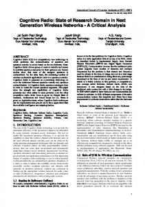
Figure 1: When limiting the scanning range, additional cohesion and collision avoidance rules can be used to restore the swarming behavior. ance. The signal strength from the radio’s own and a foreign swarm were weighted equally (except the sign), however signals introduced by the jammer were penalized by a factor of 10, modeling a very timid behavior for the stark influences introduced by the jammer. The radios’ transmit power was constant throughout the simulation. Each radio was set to a certain frequency that each radio could change at its own discretion once every epoch. The frequencies were assumed to be adjacent, but non-overlapping channels as in 802.11b. Each radio could only see and observe the nodes that are within the 150 meter range of itself and had to make decisions based only on its local view of the network environment and must not explicitly exchange status or configuration information with any other node. Further, each radio did not have a full local view of its surroundings, but could only scan a certain part of the spectrum at any time. If a given radio p is set to frequency fp , it can only see nodes on the two upper and lower adjacent channels, i.e. (fp − 2, ...fp , ...fp + 2). This extra requirement was introduced for technical considerations, as a CR should not spend most of its time/energy scanning and be equipped with low cost hardware that could only scan a small number of frequencies at a time. For simplicity in this set of experiments, we assumed symmetrical links and fixed power output and limited a CR only to avoid interference by switching its transmit frequency to eliminate the effects of multi-factor adaptivity for the analysis. The simulator was written in Java, using the Java pseudo random number generator (PRNG) with a cycle length of 232 . All sources of randomness were drawn from a dedicated PRNG that was initialized appropriately in each scenario to achieve a random but reproducible environment. As mentioned above, in this CR swarm model we diverged from the original preconditions of the swarm algorithm by limiting each entity’s scanning window to five frequencies. By restricting to detect its peers only within a certain distance and only on a subset of frequencies, we added additional complexity to the problem as each CR now only has a partial view of its local surroundings. In the original domain, this would mean that a fish would only have 160 degree vision4 and could only see its neighbors when they are within a certain distance and swimming in this 160 degree window as shown in Figure 1. Clearly, this restricted vision would make it more difficult for a fish to find and stay close with its school. To overcome this additional, artificial technical requirement not present in the original domain, we added three 4

If we scan only 5 frequencies out of 11 for 802.11.

B A

B

freq = 4

J2 freq = 4

freq = 4

freq = 4

A

D

freq = 4

E

freq = 4

C

freq = 4

G

C

freq = 4

J1 freq = 5

freq = 5

freq = 5

Figure 3: Following Temporary visitors

E

freq = 5

Figure 2: Swarms can converge to subgraphs if not prevented by the cohesion rule. additional cohesion and one collision avoidance rule5 that would allow the CR network to find its peers, stabilize quickly and not form subgraphs even though each node could only make a partial scan of its local surroundings at a time. The need for the extra cohesion and collision avoidance rules becomes evident when we transfer a limited CR back to the original domain of schooling fish as shown in Figure 1. Cohesion-II: Look for others. When a node does not see any other node within each range at its own frequency ± 2, it scans the whole spectrum and selects that frequency on which most of its peers are present. We determine presence by the ability to decode packets from other stations. This could be done less computationally expensive by looking at the power level on a particular channel. In this work however, we did not explore this method. This rule is of importance when a new node appears and must join an existing network, or when a bridge node providing the only connection to the network was jammed and switched to a frequency that is outside of the now disconnected node’s frequency scanning range. Intuitively, this would mean that a fish continues turning until it can see another peer. Cohesion-III: If a peer does not come, go to it yourself. In situations where networks are interfered with by multiple jammers from different angles, a network driven by the swarm algorithm can converge to local stable states, but remain unconnected as a whole. Figure 2 shows such a situation: Nodes A, B, and C are in range of each other and have converged to frequency 4. Nodes D, E, and F are also in range of each other and have agreed on frequency 5. While node C can see node D on the adjacent frequency 5, node C also senses the jammer J1 on frequency 5, and decides this frequency is inferior from its perspective and therefore does not switch to frequency 5 by itself, which would make nodes A and B switch to frequency 5 as well. The same situation exists for node D. It senses node C and the jammer J2 on frequency 4 and therefore does not make a change to, from its perspective inferior, frequency 4 which would then trigger E and F to also switch to 4. Cohesion rule II addresses this forming of subgraphs. A node i of a stable network that sees another peer j in range, but j does not switch to i’s frequency after a certain number of epochs, i will assume that from j’s perspective j’s frequency is better than i’s. In that situation, i will make a switch to j’s frequency and, if equal or better, remain on 5

freq = 9

freq = 9

F

D

F

denoted as Cohesion-II/III/IV and Collision Avoidance-II

j’s frequency. If i remains, this will trigger the remaining nodes of i’s network to also switch to the new frequency and the two subgraphs will merge. In a fish example, if a fish inside a school sees another school at a distance which does not come any closer, it will itself move towards the remote school and drag its own school along. Cohesion-IV: Follow temporary visitors. Consider the situation depicted in Figure 3. After a sequence of interference avoidance actions, nodes A, B, C and D form a stable network on frequency 4. Nodes F and G detected each other on frequency 9. Even though F is theoretically in range of C and D, it does not break the connection with G but stays on frequency 9 as F does not have any information about the total number of nodes in its network and has found a peer in G. After a while, node E (which might have just gotten initialized, or after a jamming attack ended up as an isolated node) is scanning frequencies and briefly switches to frequency 4. As it continues scanning and associates with other peers in range, it finally decides to remain on frequency 9 as there are more peers in its proximity (F and G). Node D noticed earlier that E was joining their frequency, but then left. Since it cannot see E in its limited frequency scanning window, it assumes that E is either dead or has found a better choice than D’s frequency. If E therefore does not return after a while, D also starts scanning the whole spectrum, despite the fact that D is a member of a stable network. Once it finds E and F on the new frequency, it also remains on frequency 9 and drags A, B and C along because they are triggered to switch by the same rule. Explained in a fish example, a fish would turn to look for a peer if the peer briefly was in sight but never appeared later again. Collision Avoidance-II: Leave noisy environments. If a peer’s network has converged to a stable state and no peers on different frequencies were ever visible that would trigger the rules Cohesion-II or Cohesion-III, a node should temporarily check if the background noise is lower on any other frequency than its current one. It will then switch to the frequency with the lower background noise and trigger the cohesion actions so all nodes in the network will rendezvous on the frequency with less noise.

4.

EVALUATION

When proposing a new algorithm, it is a challenging task to create a variety of scenarios that will reflect actual conditions that the algorithm will face in practice and not overestimate the benefit of a proposed algorithm by choosing an unrepresentative sample set. In order to avoid designing evaluation test scenarios that bias in favor of our algorithm, we created a benchmarking application that would create and evaluate test scenarios randomly.

1.0

Swarm (p=1)

0.6

Swarm (p=1)

0.2

0.4

Percent of Scenarios

0.8

0.8 0.6 0.4

Percent of Scenarios

Control-8

0.2

Control-8 0.0

For our evaluation, we randomly generated 10,000 test scenarios with 5 networks each containing 5, 10, 20, 30, 50 and 70 nodes, resulting in a total of 60,000 scenarios. In each scenario all nodes were placed randomly on a 300 by 300 meter plane such that every node was part of a connected, but not too densely connected network. For scenarios where each network contained 5, 10, or 20 nodes, each node had to be in range of a least 1, but not more than 3 other nodes of its own network ((1,3)-connectivity). For 30 and 50 nodes, we required (1,9)-connectivity and for 70 nodes, (1,20)-connectivity. Each node was initialized to a random frequency setting. Since all nodes started at the same time with a random initialization, each algorithm was given up to 500 epochs initialization to build all its necessary data structures and (for the centralized control algorithm) exchange network status information to reach steady-state. At epoch 500, a jammer was placed in the network. The location was chosen so that at least 10% of all nodes in the networks were in its transmission range. The jammer’s frequency was set to the frequency that most nodes within its range used for transmission at epoch 0. However, the control channel for the centralized approach was never jammed and was set to not encounter congestion at any time. We recognize this is acting in favor of the centralized control and not a realistic scenario. After the scenarios containing the nodes’ physical position and initial frequency assignment and the jammer’s position and frequency were generated, each control algorithm was evaluated with each of the 60,000 scenarios. For each of these runs, we recorded the networks’ overall performance for every epoch, whether each network had achieved full connectivity, and at which epoch the control algorithm converged to the final, stable solution. For the swarm algorithm, we assumed that in a certain epoch nodes were active with a certain probability. If a node decided to be active during a time interval, it was visible to other nodes around it. Otherwise, its neighbors did not have any information about this node. For the analysis of performance, convergence, and disconnected networks in Sections 4.2, 4.3 and 4.4, we assumed a probability of p=0.25 and/or p=1 that nodes were active. In Section 4.5 however, we explore how the swarm behavior changes for a variety of probabilities with p={0.25, 0.5, 0.6, 0.7, 0.8, 0.85, 0.9, 0.95, 1}. To benchmark the performance of the swarming approach, we implemented a second control algorithm. This algorithm provided a central authority that was in range of every other node, received local observations from nodes and issued (based on the current global knowledge) the best possible configuration to each node. These status and configuration messages were transmitted on a different channel that was fixed throughout the simulation. Such a control channel can nevertheless not transport an unlimited amount of communication messages. While the actual capacity would be limited in practice due to back-off, transmit, decoding and processing times, network topology would further limit the amount of communication messages. As in a typical deployment, not every node would be in range of the central authority. Thus, packets would need to be routed by nodes along the way and nodes would consume overhead air time for the relaying of packets. To account for this bottleneck we limited the number of

1.0

Setup of the Evaluation

0.0

4.1

0.0

0.2

0.4

0.6

0.8

1.0

Percentage of best scenario's result reached in epoch 10

(a) after in steady state

0.0

0.2

0.4

0.6

0.8

1.0

Percentage of bests scenario's result reached in epoch 50

(b) after initialization

Figure 4: Performance Comparison between Swarm (p=1) and Control-8 messages that could be transmitted to and from the central authority during every epoch. We assumed a 50 ms interval for every epoch, which would provide the Swarm enough time for scanning five frequencies and the central authority enough time to send and receive about 16-17 messages.6 To quantify the lost capacity due to routing control messages, we calculated the average number of hops that it would take from one node to get to any other node for the 10,000 scenarios, since theoretically every deployed node could act as the controlling agent. As it would take on average more than 2 hops7 (thus relayed messages) to distribute status and configuration information, we allowed the central authority to receive and send 8 and 20 messages within each epoch, which are labeled in the following sections as Control8 and Control-20, respectively, and are upper bounds for the behavior of the centralized control algorithm, modeling a two-hop routing and a no-routing case. /Users/christian

4.2

Performance

Figure 4 shows the performance of the Swarm (p=1) and Control-8 algorithm as a cumulative distribution function (CDF). Due to space restrictions, we are discussing only two scenarios that illustrate the performance of the two algorithms. Figure 4(b) displays the performance of both algorithms at epoch 50 during the initialization period. In this part of the simulation, the algorithms started from a random initialization and needed to converge to a common configuration without the presence of a jammer. Figure 4(b) shows the percentage of the best possible result for this scenario achieved at epoch 50 in the initialization period. One can see that the Swarm approach outperforms the Control-8 algorithm in the case where many configurations must be performed in parallel as the algorithms started from a random but identical initialization: In 90% of the least scoring scenarios, the Control-8 algorithm has only achieved about 10% of its best possible performance at the end of the initialization period, while the Swarm (p=1) algorithm has achieved about 80% of its final performance. As discussed before, in epoch 500 a jammer appears that will jam 10% of the network after the algorithms have reached steady state. Figure 4(a) shows the performance of the algorithms 10 epochs after being jammed, measured as a percentage of the final performance at the end of the adapta6 It takes about 3 ms to send a 200 byte packet on 802.11b with 1 Mbps. 7 1.4 messages in a 5 node, 2 messages in a 10 node, 2.8 messages in a 20 node network etc.

Table 1: Convergence Time # of Nodes 5 10 20 30 50 70

Swarm (1) avg/std 8.1 / 27.1 17.4 / 46.8 57.0 / 133.5 37.2 / 109.1 43.6 / 117.7 71.6 / 162.0

Swarm (0.25) avg/std 25.6 / 79.5 15.6 / 26.9 17.0 / 33.1 17.3 / 46.4 32.5 / 91.6 83.6 / 152.2

Control-8 avg/std 17.5 / 9.8 26.2 / 14.3 61.2 / 21.7 91.2 / 57.5 208.1 / 154.8 286.2 / 123.7

Control-20 avg/std 4.4 / 2.4 7.0 / 3.3 17.2 / 10.6 26.2 / 7.3 57.8 / 45.2 183.2 / 117.7

tion. Both algorithms have achieved a high percentage early on; in 80% of the runs both algorithms achieve at least 95% of their final result already in epoch 10, however the swarm algorithm slightly underperforms in this scenario.

4.3

Convergence Time

Table 1 shows the convergence time on instances of 5, 10, 20, 30, 50 and 70 nodes for the Swarm (p=0.25), Swarm (p=1.0), Control-8 and Control-20 algorithms. As expected Control-20 clearly outperforms Control-8 since its higher communication rate with the nodes lets it configure the nodes faster and can adapt more efficiently to the jammer’s influence. Therefore, both the average time to converge and the standard deviation (std) is lower for Control-20 in comparison to Control-8. When doing a pair-wise comparison between the four algorithms, one can see that for small instances from 5 to 30 nodes, Control-20 clearly outperforms the Swarm algorithms, while Control-8 is outperformed by at least one of the two Swarm algorithms. In all these cases the difference is not statistically significant, due to the large standard deviation. This fast convergence and the improvement in iterations can be seen in Figure 5. The number of total iterations to final convergence, however, grows faster for the centralized control algorithms than for the swarm approach, so that Control-8 is outperformed by both swarms for 20 nodes and Control-20 for 50 nodes. For growing network sizes the amount of communication between the central coordinator and the nodes also grows linearly while the number of slots available for communication with the nodes remains constant. Therefore, it takes more iterations to reach all nodes and to react to the jammer’s and other networks’ influences as can be seen in Figure 6. Figures 5 and 6 also show the reason for the Swarm’s large standard deviation on its convergence time and why for large instances the Swarm approach might be a better choice. The randomness in the Swarm algorithm8 lets some instances converge only after a long time. This happens for example when nodes in disconnected networks repeatedly make local actions to rendezvous with a neighbor while that neighbor simultaneously makes a similar, but counter action from a global perspective. These late converging instances in Figures 5(a)(b) and 6(a)(b) drive the average convergence time and especially its std up. However, in the majority of runs (especially for larger instances) the Swarm algorithms finish significantly earlier than Control-8 and Control-20.

4.4

Disconnected Networks

A similar pattern exists for the connectivity of networks. After each epoch, we evaluated whether the current network configuration realizes a fully connected network, i.e. if every node in a given network can talk to every other node 8 For example by not looking at its neighbors in a predefined, specific order.

on the same frequency. Table 4.4 lists the average number of disconnected networks and the standard deviation that occurred in the 500 epochs reconfiguration time after the jammer’s appearance for the five networks. Both the average number of disconnected network states and its standard deviation is lower for Control-8 and Control20 when compared to those of the Swarms for network sizes up to 30 nodes (except for Swarm p=1 and 5 nodes). As the number of nodes in the network grows, the centralized algorithms reach a tipping point. For 50 nodes, the Control-8 algorithm’s connectivity rapidly drops. As shown in Figure 8(c), in none of the 10,000 scenarios containing 50 nodes does the Control-8 algorithm configure the network fast enough that less than 50 disconnected network states occur, and more than half the scenarios have more than 200 epochs of unconnected network states. Similarly, the Control-20 algorithm also shows a significant number of large disconnected states, which more dramatically increases once the network size is increased to 70. The relatively high standard deviation for the Swarm algorithms can again be explained by the small number of “late convergers” (see Figures 7 and 8), while in the majority of runs the Swarm algorithms finishes within the first 30-80 epochs.

4.5

Activeness of Nodes

Besides network topology and network size, the performance of network configuration algorithms also depend on the number of nodes actually active inside the network at a certain time. If a node is not active in a centralized scenario, it cannot exchange network status and configuration. If a node is not active for the swarm scenario, its neighbors are not aware of it and cannot change their configuration based on its presence. To quantify the impact of the activeness of a network’s nodes on the convergence of the algorithm, we simulated 500 network scenarios with 8 different activation levels and with 6 different network sizes. For each of the scenario, we configured the nodes that they send with probabilities of 0.25, 0.5, 0.6, 0.7, 0.8, 0.85, 0.9, 0.95 and 1 and placed 5, 10, 20, 30, 50, and 70 nodes in each of the 5 networks. The result of these 24,000 test cases is shown in Figure 9. As can be seen in the Figure, the swarm algorithm converges at similar times for all levels of activeness and network sizes. The small variations in average convergence time result from outliers as discussed in Section 4.3 and tabulated (for 10,000 scenarios) in Table 1. The reason for the similar performance results from the interplay of the four cohesion rules: As the number of active nodes in a scenario decreases, the overall network looses some cohesion as the sleeping nodes cannot be seen and are not taken into account when the nodes are converging to a common configuration. This lack of convergence due to the Cohesion-I rule (adjust your configuration to that of your neighbors) however # of Nodes 5 10 20 30 50 70

Swarm (1) avg/std 8.1 / 22.5 27.0 / 68.5 50.1 / 122.8 52.6 / 161.1 64.7 / 196.1 87.3 / 203.7

Swarm (0.25) avg/std 16.2 / 74.6 21.5 / 37.7 36.1 / 87.5 39.9 / 129.6 76.6 / 246.6 207.4 / 425.1

Control-8 avg/std 10.6 / 10.7 14.2 / 15.2 21.6 / 16.0 28.5 / 0.4 144.5 / 133.4 324.6 / 95.9

Control-20 avg/std 2.6 / 2.6 3.9 / 3.5 11.8 / 10.8 8.2 / 4.9 42.4 / 37.7 247.0 / 138.0

Table 2: Number of Disconnected Network States

700

800

900

1000

600

700

800

900

1000

600

(a) Swarm (1) with 10 nodes

700

800

900

1.0 0.8 0.6 0.4 0.2

Percentage of Scenarios converged 500

epoch

0.0

1.0 0.8 0.6 0.4 0.2

Percentage of Scenarios converged 500

epoch

0.0

1.0 0.8 0.6 0.4 0.2

Percentage of Scenarios converged 600

0.0

1.0 0.8 0.6 0.4 0.2

Percentage of Scenarios converged

0.0 500

1000

500

600

epoch

(b) Swarm (0.25) with 10 nodes

700

800

900

1000

epoch

(c) Control-8 with 10 nodes

(d) Control-20 with 10 nodes

600

700

800

900

1000

600

700

800

900

1000

700

800

900

1000

epoch

(b) Swarm (0.25) with 50 nodes

(c) Control-8 with 50 nodes

1.0 0.8 0.6 0.4 0.2

Percentage of Scenarios converged 600

0.0

1.0 0.8 0.6 0.4 500

epoch

(a) Swarm (1) with 50 nodes

0.2

Percentage of Scenarios converged 500

epoch

0.0

1.0 0.8 0.6 0.4 0.2

Percentage of Scenarios converged 500

0.0

1.0 0.8 0.6 0.4 0.2 0.0

Percentage of Scenarios converged

Figure 5: Convergence time to a final solution for Swarm, Control-8/-20 for five networks with 10 nodes each

500

600

700

800

While in a medium jamming context (10% of nodes affected) the swarm algorithm achieves nearly the same results as the best-possible algorithm using global knowledge in terms of performance, in a scenario where much adaptation needs to be done, i.e. after a global initialization (where 100% of nodes need to be coordinated) the swarm clearly outperforms a centralized control. Due to its multiple coherence functions, the swarm algorithm is independent of nodes activeness and also stabilizes in situations where only a few nodes are active at a time.

90 Avg. Convergence

80 70 60 50 40 30 20 10 0 5

10

20

30

50

70

Nodes in Swarm 1

0.95

0.9

0.85

0.8

0.7

0.6

0.5

0.25

5.

CONCLUSIONS

is counterbalanced by the Cohesion-II, -III and -IV rules. When less nodes are active, these nodes can converge quicker to a common configuration. When additional nodes become also active, the awakening nodes then see a few already converged networks and join these (Cohesion-II). When only a few these converged networks exists instead of many, these can also then come to a common configuration faster (following Cohesion-III/Cohesion-IV).

In this paper, we have introduced and transferred the concept of emergent behavior as found in schools of fish and flocks of birds to the domain of CR networks. We have shown that the underlying mechanism can help a decentralized network to converge to a common configuration and adapt to outside influences quickly. Our results further showed that for growing network sizes, algorithms based on centralized control can reach limitations which are overcome by the algorithm based on emergent behavior. The proposed algorithm scales well to large network sizes and is insensitive to the level of activeness of its network’s nodes.

4.6

6.

Figure 9: Comparison of swarm behavior convergence for various node activeness probabilities

Summary

As discussed in the previous sections, the decentralized swarming approach provides competitive results in terms of overall performance, convergence time and connectivity of the network when benchmarked against a centralized control algorithm without requiring the exchange of explicit configuration messages. The swarm algorithm scales better than a centralized one and outperforms in medium size scenarios in respect to convergence time and network connectivity.

1000

(d) Control-20 with 50 nodes

Figure 6: Convergence time to a final solution for Swarm, Control-8/-20 for five networks with 50 nodes each 100

900

epoch

REFERENCES

[1] M. Bandholz, J. Riihij¨ arvi, and P. M¨ ah¨ onen. Unified layer-2 triggers and application-aware motifications. In IWCMC ’06: Proceeding of the 2006 international conference on Communications and mobile computing, pages 1447–1452, New York, NY, USA, 2006. ACM Press. [2] X. Cui, C. T.Hardin, R. K. Ragade, and A. S. Elmaghraby. A swarm approach for emission sources

100

200

300

400

500

0

disconnected networks

100

200

300

400

500

1.0 0.8 0.6 0.4 0.0 0

disconnected networks

(a) Swarm (1) with 10 nodes

0.2

Percentage of Scenarios

1.0 0.8 0.6 0.4 0.0

0.2

Percentage of Scenarios

1.0 0.8 0.6 0.4 0.0

0.2

Percentage of Scenarios

1.0 0.8 0.6 0.4 0.2

Percentage of Scenarios

0.0 0

100

200

300

400

500

0

disconnected networks

(b) Swarm (0.25) with 10 nodes

100

200

300

400

500

disconnected networks

(c) Control-8 with 10 nodes

(d) Control-20 with 10 nodes

0

100

200

300

400

500

disconnected networks

(a) Swarm (1) with 50 nodes

0

100

200

300

400

500

disconnected networks

(b) Swarm (0.25) with 50 nodes

1.0 0.8 0.6 0.4 0.0

0.2

Percentage of Scenarios

1.0 0.8 0.6 0.4 0.0

0.2

Percentage of Scenarios

0.8 0.6 0.4 0.0

0.2

Percentage of Scenarios

0.8 0.6 0.4 0.2 0.0

Percentage of Scenarios

1.0

1.0

Figure 7: Disconnected networks until a final solution for Swarm, Control-8/-20 for five networks with 10 nodes each

0

100

200

300

400

500

disconnected networks

(c) Control-8 with 50 nodes

0

100

200

300

[3]

[4]

[5] [6]

[7]

[8]

[9]

500

(d) Control-20 with 50 nodes

Figure 8: Disconnected networks until a final solution for Swarm, Control-8/-20 for five networks with 50 nodes each localization. In Proceedings of the 16th IEEE International Conference on Tools with Artificial Intelligence (ICTAI 2004, 2004. M. Danzeisen, T. Braun, S. Winiker, and D. Rodellar. Implementation of a cellular framework for spontaneous network establishment. In WCNC 2005, 2005. K. Kelly. Out of control: the new biology of machines, social systems and the economic world. Addison-Wesley, 1994. W. C. Lee. Mobile design fundamentals. John Wiley, 1991. N. Nie and C. Comaniciu. Adaptive channel allocation spectrum etiquette for cognitive radio networks. ACM MONET (Mobile Networks and Applications), 11(6):779–797, 2006. K. Oikonomou, A. Vaios, S. Simoens, P. Pellati, and I. Stavrakakis. A centralized ad-hoc network architecture (cana) based on enhanced hiperlan/2. In The 14th IEEE International Symposium on Personal, Indoor and Mobile Radio Communication Proceesings, 2003. H. V. D. Parunak, M. Purcell, and R. O’Connell. Digital pheromones for autonomous coordination of swarming uavs. In American Institute of Aeronautics and Astronautics, 2002. D. Petrovich. Structural emergence and the collaborative behavior of autonomous nano-satellites. Master’s thesis, Air Force Institute of Technology, 1999.

400

disconnected networks

[10] C. Reynolds. Flocks, herds, and schools: a distributed behavioural model. Computer graphics, 21(25-34), 1987. [11] T. W. Rondeau, B. Le, C. J. Rieser, and C. W. Bostian. “cognitive radios with genetic algorithms: Intelligent control of software defined radios. In SDR Forum Technical Conference, 2004. [12] E. Sahin and N. R. Franks. Measurement of space: From ants to robots. In Proceedings of WGW 2002: EPSRC/BBSRC International Workshop Biologically-Inspired Robotics, 2002. [13] R. Schoonderwoerd, O. Holland, and J. Bruten. Ant-like agents for load balancing in telecommunications networks. In AGENTS ’97: Proceedings of the first international conference on Autonomous agents, pages 209–216, New York, NY, USA, 1997. ACM Press. [14] T. Weingart, G. V. Yee, D. Sicker, and D. Grunwald. A dynamic cognitive radio configuration algorithm. IEEE Communications, 2006. [15] G. Werner-Allen, G. Tewari, A. Patel, M. Welsh, and R. Nagpal. Firefly-inspired sensor network synchronicity with realistic radio effects. In Proceedings of the 2th ACM Conference on Embedded Networked Sensor Systems (SenSYS), 2005. [16] R. Winter, J. Schiller, N. Nikaein, and C. Bonnet. Crosstalk: Cross-layer decision support based on global knowledge. IEEE Communications Magazine, 44(1):93–99, 2006.