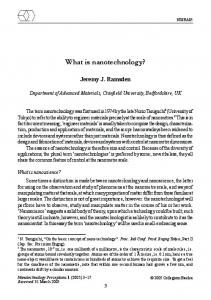
A topographic map (Bingham Canyon area in Utah) with contour lines spaced in a ... lighted by bold green lines. b is at the bottom of the Bingham Canyon Mine, ...
What is in a Contour Map? A Region-based Logical Formalization of Contour Semantics Torsten Hahmann1 and E. Lynn Usery2 1
2
National Center for Geographic Information and Analysis, School of Computing and Information Science, University of Maine, Orono, ME 04469, USA Center of Excellence for Geospatial Information Science, U.S. Geological Survey, Rolla, MO 65401, USA
Abstract. Contours maps (such as topographic maps) compress the information of a function over a two-dimensional area into a discrete set of closed lines that connect points of equal value (isolines), striking a fine balance between expressiveness and cognitive simplicity. They allow humans to perform many common sense reasoning tasks about the underlying function (e.g. elevation). This paper analyses and formalizes contour semantics in a first-order logic ontology that forms the basis for enabling computational common sense reasoning about contour information. The elicited contour semantics comprises four key concepts – contour regions, contour lines, contour values, and contour sets – and their subclasses and associated relations, which are grounded in an existing qualitative spatial ontology. All concepts and relations are illustrated and motivated by physical-geographic features identifiable on topographic contour maps. The encoding of the semantics of contour concepts in first-order logic and a derived conceptual model as basis for an OWL ontology lay the foundation for fully automated, semantically-aware qualitative and quantitative reasoning about contours. Keywords: contour maps, isolines, knowledge representation, first-order logic, spatial ontology, region-based space, naive geography, physical reasoning
1
Introduction
Contour maps effectively convey information about measures taken at spatial locations within a bounded or unbounded region of space, such as elevation information on a topographical surface, bathymetric information about the depths of lakes and seas, or meteorological information, e.g., barometric pressure or annual rainfall. 3 A contour map compactly represents such a function of space by reducing it to a small set of contours (also called contour lines or isolines), each of which has an associated contour value. Each contour separates points in the underlying space based on whether their function value is below or above the contour value. For example, contours on topographic maps (see Fig. 1) separate the areas where the elevation is higher than the contour value from those where the elevation is lower than the contour value. Thereby, contours reduce the complexity of the underlying field by extracting a representation 3
Such measures form a field when the space is unbounded. We use the term field more loosely, including both bounded and unbounded variants.
that is conceptually simple enough to effectively communicate the encoded information to humans, yet sufficiently expressive and detailed so that humans can use it to answer many common sense questions about the underlying field. The idea of contours dates, at least, back to the abstractions that Charles Hutton [10] employed in the 18th century to estimate the mean density of the Earth; even earlier uses are discussed in [17]. The earliest USGS topographic maps from the 1880s already employ contours to visualize terrain elevation [24]. Despite the widespread use of contours by humans for geospatial data visualization and analysis, representations for contours are missing from all currently available geospatial data standards, including the OGC Reference Model [15]4 , and have not been utilized for machine-based naive geographical (in the sense of [4]) or physical-geographical processing and reasoning. Many common sense questions, such as identifying high points in a terrain, finding paths that minimize elevation differences, or locating where water flows and collects, could be directly answered by a automated deduction system, e.g. a theorem prover or similar inference mechanism, from a declarative specification of a field’s contours as facts about their qualitative spatial relationships on top of the proposed ontology. It could completely forego the process of having to produce a (printed or digital) map image and does not need to employ the full dataset of the (possibly unknown) underlying field nor full-fledged three-dimensional spatial algorithms. Encoding the knowledge represented by a field in a computer-interpretable format that captures the essence of contour maps opens up many possibilities for qualitative reasoning [3, 9] that goes beyond the most simplistic qualitative formalisms concerned only with abstract regions of space. 1.1
Objective
The objective of this paper is to lay the semantic foundations that will enable computers to perform such common sense reasoning with contour information without human interaction. More specifically, we investigate the use of a region-based formalism of contour semantics, building on existing ontologies of qualitative space [7] and measured quantities [20], and formalizing the identified key concepts and relations explicitly in a first-order logical ontology. The resulting ontology can facilitate machine processing and reasoning of contour information, either directly by utilizing automated theorem provers, or indirectly by deriving lightweight versions of the ontology. Ultimately, we want an automated reasoner to be able to utilize contour information encoded in the ontology to answer simple qualitative or Boolean queries such as: – Is the path along a given two-dimensional vector (in the underlying, implicit field) relatively flat, ascending, descending, or a combination thereof? – Is there a path between two points that does not involve a change in elevation? – Which of two areas has a greater maximal elevation? – Which of two areas has a greater roughness (turtourocity)? It turns out that basic integer operations and spatial sums suffice to capture the quantitative aspects of contour semantics (to constrain contour values and points values). Including these operations in the formalization of contour semantics greatly increases the utility and expressiveness of the otherwise purely qualitative representation. 4
OGC’s reference model and more specific standards such as GeoSPARQL and GML include coverage data types to represent fields, but offer no way of representing fields using contours.
Fig. 1. A topographic map (Bingham Canyon area in Utah) with contour lines spaced in a contour interval of 50 feet apart. The contours e–o denote ascending contours, while the hachured contours a–d denote descending contours. All named contours are completely or partially highlighted by bold green lines. b is at the bottom of the Bingham Canyon Mine, an open-pit copper mine in operation since the beginning of the 20th century. To the west (left-hand side), the terrain rises steeply (along the superimposed line that runs perpendicular to contours), with Clipper Peak (n) reaching above 9200 feet. See the text for examples and more explanations.
Our specific contributions are: (1) analyzing whether a contour region is an adequate primitive notion for formalizing contour semantics; (2) formalizing contour semantics as a region-based first-order ontology using a small set of contour-related primitives (contour set, ascending and descending contour regions, and a relation between contour regions and their boundary values); (3) relating the contour values associated with contour regions to measures at individual points; (4) identifying the additional quantitative operations that are required to support reasoning about contours; (5) mathematically characterizing important classes of contour sets and maps; and (6) deriving a lightweight conceptual model from the first-order formalization. 1.2
Background
While much work has been done to automatically derive contour maps from threedimensional data, e.g. terrain data [18] as represented in Digital Elevation Models (DEM), less focus has been put on making such derived contour maps available for automated reasoning. Early work on digital representations of contour maps [1, 6, 11, 13] has focused on utilizing tree structures to identify pits, peaks, saddles, ridges and similar topographic features, but has not attempted to formalize contour semantics. Moreover, the developed data structures, so-called contour trees, emphasize the nesting and adjacency relationship between contour lines and have been effective for surface and feature extraction, but are conceptually difficult to reason with. Our objective is to devise a conceptually and mathematically simpler representation of contours by using a
region-based approach that emphasizes the regions enclosed by contours over the contours themselves. This will enable the development of an ontology of contour semantics that extends qualitative, mereotopology-based representations of space, e.g. [2, 5, 9, 19], while also being able to define contour lines and the relationships among contour lines as well as between contour lines and the regions they bound. This would not be possible in the simpler formalisms from [2, 5, 19], that do not capture relationships between spatial entities of different dimensions, such as between regions and curves. As basis for such a region-based formalization of contour semantics, we focus on the ontological concepts that underlie contour map conceptualizations (the idea of a set of nested contours, wherein all contours are closed curves, i.e. curves without endpoints) and not contour map depictions (the visualization of a typically rectangular portion of a contour map conceptualization wherein contours may end at the edge of a map). Each contour conceptualization is treated as a set of holeless contour regions (each bounded by a contour) on a two-dimensional plane, related by spatial containment (one contour region being a subregion of another one). We are agnostic about how the contour representation is obtained in the first place: it may be derived from a primary data source such as a DEM or it may be the only available source, as is the case for many historic maps or maps sketched by humans. But even when the primary data are available for querying, a contour representation may provide a cognitively simpler, yet semantically rich model for human-computer interaction about the underlying field. We are at no point concerned with recovering the original field through approximations/interpolations from a contour conceptualization. 1.3
The Underlying Multidimensional Qualitative Spatial Ontology
The presented formalization of contour semantics reuses the theory CODIB from [7, 8] that formalizes basic qualitative spatial relations between abstract spatial regions (subsequently we drop the implicit qualifier “abstract”) of different dimensions, including points, linear features (curve and line segments and complex curve/line configurations), areal regions and voluminous regions. CODIB is briefly reviewed here; Table 1 summarizes all relevant predicates and their intended interpretations with the full details available in [7]. It is formalized using the basic spatial relation of containment, Cont(x, y), meaning that the spatial region x is spatially contained (a subregion of) in the spatial region y – independent of the dimensions of x and y (x can, of course, never have a greater dimension than y), and BCont(x, y) meaning that x is contained in the boundary bd(y) of y and thus necessarily of a lower dimension than y. Independent of their dimension, all spatial regions are topologically closed, that is, every point on their boundary is contained in the set. Additionally, a predicate ≤dim (x, y) relatively compares the dimensions of two arbitrary spatial regions. The following kinds of spatial regions can be defined and distinguished based on the spatial relations they partake in and their relative dimensions: Point(x), Curve(x), and ArealRegion(x). We particularly require simple loop curves, curves that form a loop, and closed areal regions, which are either closed manifolds (like a sphere) or regions bounded by a simple loop curve (manifolds with boundaries). Because all spatial regions are topologically closed, curves that have endpoints always include their endpoints (a loop curve or infinite curve without endpoints as well as rays with a single
Table 1. Summary of the spatial concepts and relations from [7] and their information definitions that are used in the formalization of contour semantics. spatial predicate
informal definition
Cont(x, y)
x is spatially contained in y (all points in x are also in y) independent of the dimensions of x and y PO(x, y) x and y spatially overlap, that is, their intersection is non-empty. Cont(x, y) and Cont(y, x) are specializations of PO(x, y) BCont(x, y) x is boundary-contained in y; that is, Cont(x, bd(y)) holds TCont(x, y) x is spatially contained in y and part (either a point or a segment) of the boundary of x is contained in the boundary of y Con(x) x is a self-connected spatial region, that is, every part of x is connected to its complement Point(x) x is a point, i.e, an indivisible zero-dimensional spatial region Curve(x) x is a curve, i.e., a one-dimensional spatial region (which includes straight lines as well as straight and curved line segments) SimpleLoopCurve(x) x is a curve that represents a closed manifold, i.e., it is selfconnected, not self-intersecting and has no branching points ArealRegion(x) x is a two-dimensional spatial region ClosedArealRegion(x) x is a two-dimensional spatial region that represents a closed manifold or a manifold with boundary bounded by a simple loop curve
endpoint are still topologically closed) and areal regions always include their boundary curve(s) if one exists (a plane or the surface of a sphere without boundaries as well as half-planes with a partial boundary are still topologically closed). The formalization in CODIB makes no assumption about the specific digital representations of spatial regions. For example, arbitrary curves may be represented as polylines, as sets of Bezier curves, or in other ways. The actual representation does not impact the semantic constraints that they must adhere to. This also holds true for the proposed formalization of contour semantics: it is not tied to whether the underlying, often implicit, field is encoded using a DEM, TIN, a simple raster representation, a vector representation, or any other suitable format.
2
The Basic Contour Concepts and Their Formalization
We are interested in the most general, yet essential semantics for representing a field as a contour map independent of what kind of measure the field represents. However, we will use elevation contours as found on topographic maps to motivate and illustrate the presented axioms and definitions. Nevertheless, we intend our ontology to apply equally to all kinds of contour maps with other kinds of measures such as bathymetric elevation, barometric pressure, temperature, or precipitation (rainfall/snow). The ontology also applies to interpolated measures such as population density, household income, or crime rate, which cannot be directly measured at individual points and whose contour lines are referred to as isopleths for that reason. The only constraint we impose on the underlying field is that its values form a continuous surface, ruling out, for example, the existence of overhanging rock faces that could yield multiple contours. The underlying field is
not required to be functional (single-valued), that is, we allow “vertical cliffs” that yield more than a single elevation value at a point, though these must be continuous in the previous sense in order to clearly indicate an instantaneous rise or drop in value. For our formalization, we will treat contour regions as abstract spatial regions that are distinct from physical entities, such as an actual mountain or a depression, and from other nonphysical entities, such as a conceptual or real map of population density, that it may represent. Contour regions are abstract spatial regions that describe the spatial extent (or parts thereof) of the represented mountain or depression as a (simplified) mathematical abstraction. Contour regions differ from arbitrary closed areal region (the subclass of abstract spatial regions they specialize) in that they must be associated to a contour value that describes a physical property of the represented physical object or field within that region. So in order to distinguish them from other closed areal regions, we introduce a new primitive notion. Analogously, we must distinguish contour lines from arbitrary simple loop curves, the kind of abstract spatial regions they specialize. Multiple concepts would qualify as primitive notions, including the notions of a “contour line” (the lines usually drawn on a contour map which indicate the contour value at the points on the line), a “region of equal contour value” (the area between two “adjacent” contour lines), and of a “contour region” (the entire area enclosed by a contour line). We chose the last option as primitive for the following reasons. First, contour regions and lines are interdefinable, that is, contour lines are simply the boundaries of contour regions and contour regions are spatial regions bounded by contour lines. But by relying on contour lines as primitive makes it logically more difficult to define contour regions because contour lines separate two half-planes, whose formal distinction is nontrivial. Moreover, contour regions are spatially more well-behaved than contour lines in the sense that they have a natural spatial containment (“nesting”) relation. For the latter reason, the contour regions are also preferable over the “regions of equal contour value”, which are not spatially nested but spatially encircle one another without overlap or intersection. The spatial relationship among “regions of equal contour value” requires distinguishing the notion of “topologically inside” from “topologically outside”. Moreover, the nesting of contour regions is robust when the contour interval is changed: a finer contour interval defines regions that are spatially contained in the regions obtained using a coarser contour interval. This is not the case for the “regions of equal contour value”. Finally, contour regions are always holeless regardless of the resolution (the contour interval) of the contour map. 2.1
Contour Regions
Our new primitive spatial concept is that of a contour region, in addition to the purely spatial primitives introduced in [7, 8]). A contour region is a special kind of holeless ClosedArealRegion, a topologically closed two-dimensional (“areal”) region bounded by a single closed curve. We call the bounding curve of such a region a contour, formalized in more detail in Section 2.6. Intuitively, the contour that bounds a contour region is a curve that is both simple, i.e. without branching points, and a closed manifold, i.e. without endpoints (CR-A0)5 . While in map drawings contours may end 5
All presented axioms, definitions and theorems are first-order sentences which are implicitly universally quantified over any variables that are not explicitly quantified.
at the edge of the map, conceptually they continue beyond the visible portion of the contour map, forming a closed curve. Since the presented ontology is about the conceptualization of a contour map, not about its actual drawing, the encoding of a specific field would always result in a set of closed contours such that the outermost contours define the extent of the, possibly irregular-shaped and disconnected, conceptualized contour map. CR-A0 is included for completeness and to fully integrate the presented contour ontology with the spatial ontology CODIB [7]. However, the contour ontology can be reused without importing CODIB and all its dependencies, as long as all spatial predicates are interpreted as described informally in Table 1 and formally in [7]. (CR-A0) CR(x) → ClosedArealRegion(x) ∧ Con(x0 ) ∧ SimpleLoopCurve(bd(x)) (all contour regions are closed areal regions without holes, that is, whose complement is self-connected, bounded by a simple curve with no end- or branch points) 2.2
Contour Values
Contour regions differ from other abstract spatial regions in that they are associated with observations or measures (for the purpose of this paper, we do not distinguish between those) of a specific field’s quality, such as elevation, which could also be an interpolated, derived, estimated, or simulated quality. We call the actual measure of this quality the contour region’s contour boundary value, denoted by the relation ctrBdV (x, vx ). It expresses that vx is the measure, which we call the measured quantity, in the underlying field at every point on the boundary of contour region x. ctrBdV is a functional relation for contour regions, meaning that every contour region has exactly one contour boundary value associated with it (CV-A2, CV-A3). A contour inherits the contour boundary value from the contour region it bounds (CtrV-D). We reuse some of the core ideas from the Observation and Measurement Ontology [20] in dealing with contour values. Specifically, contour values are special kinds of measured quantities (also called observed quantities), with each such contour value being associated with some measured quality and measurement scale (CV-A4). Ontologically, measured quantities and thus contour values are qualities, which are distinct from the categories of endurants and perdurants (compare [12]). Most importantly, CVA6 captures the fundamental property that a contour’s boundary value is equivalent to the measured quantity of all point measures along its bounding contour line, which in turn allows inferring that the measured quantities along the boundary of a single contour region are constant (CV-T1)6 . (CV-A1) CR(x) → ∃vx [ctrBdV (x, vx )] (all contour regions have a contour boundary value) (CV-A2) ctrBdV (x, vx ) → CR(x) ∧ CV (vx ) (ctrBdV is a relation between contour regions and contour values) 6
We assume that any two measured quantities x and y with MQuantity(x) and MQuantity(y) can be directly compared using standard (in)equality so that the result is not a mere comparison of their numeric values (denoted by mValue(x) and mValue(y)) but takes their associated units mUnit(x) and mUnit(y) into account. E.g., if x = 1km and y = 100m, then x > y is true. All comparisons of measured quantities, even between quantities in the same unit, require a common measured qualities (mQuality(x) = mQuality(y)), e.g., both are elevations.
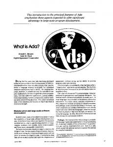
Fig. 2. The concepts of contour region and contour value in relationship to the concepts and relations concerning measures. Each contour region has a unique contour value associated to via the ctrBdV relation. Each contour value is a measured quantity or observation, which has a numerical value, a unit, a quality that is measures (such as elevation or annual precipitation), and an associated scale. Measures can also be taken at points, which are spatially related to the contour regions via the relations Cont and BCont.
(CV-A3) ctrBdV (x, v1 ) ∧ ctrBdV (x, v2 ) → v1 = v2 (each contour region has a unique contour boundary value, that is, ctrBdV is a function on the domain CR) (CV-A4) CV (x) → MQuantity(x) ∧ ∃y[mScale(x, y) ∧ OrdinalMScale(y)] (each contour value is a measured quantity that has a ordinal scale associated to it) (CV-A5) pointMQ(p, vp ) → Point(p) ∧ MQuantity(vp ) (pointMQ(p, vp ) relates a measured quantity to the point it has been measured at) (CV-A6) ctrBdV (x, vx ) ∧ pointMQ(p, vp ) ∧ mQuality(vx ) = mQuality(vp ) ∧ BCont(p, x) → vp = vx (point measures on a contour region’s boundary that measure the same quality as the contour boundary value have the same quantity as the contour boundary value) (CV-T1) ctrBdV (x, vx ) ∧ pointMQ(p, vp ) ∧ pointMQ(q, vq ) ∧ BCont(p, x) ∧ BCont(q, x) ∧ mQuality(vx ) = mQuality(vp ) = mQuality(vq ) → vp = vq (any two points on the boundary of a contour region that measure the same quality as the contour region must have the same measured value; follows from CV-A6) Contours only make sense for measured qualities associated with a scale that has a linear order defined over all possible measured values. Otherwise the nesting of contour regions bears no useful information. For example, for any two elevation measures a and b either a > b, a = b or a < b is true. Thus, contour values must have at least an ordinal scale associated with it (CV-A4). The scale is either a discrete or a continuous ordered set of values, possibly bounded by some lowest and/or highest value (e.g. no point has a precipitation less than 0 liters per m2 per year) or be unbounded. Our restriction to ordinal scales disallows representing fields of measured qualities that use nominal scales (“categorizations”, see [23]) in our ontology, because they lack clear semantics of what it entails when two contour regions are spatially nested. The semantics of special sets of contour regions defined later in the paper relies on the scale’s ordering of the associated contour values. More powerful scales, such as interval or ratio scales, specialize ordinal scale (CV-A7, CV-A8) and are thus permissible.
(CV-A7) IntervalMScale(x) → OrdinalMScale(x) (qualities measured using interval scales are a subclass of those using ordinal scales) (CV-A8) RatioMScale(x) → IntervalMScale(x) (qualities measured using ratio scales are a subclass of those using interval scales) Alternatively to aligning our formalization with the observation and measurement pattern from [20], it could also be aligned with the joint OGC-ISO standard on geographic observations and measurements [16]. The only drawback of such an alignment is that the OGC standard does not explicitly distinguish the different measurement scales on which our formalization relies. In other respects, the OGC standard offers additional modeling capabilities, such as more fine-grained classifications of observations, ways to represent dynamic (temporally changing) observations, and representation of sampling, that are unnecessary for modeling static contour maps. 2.3
Contour Sets
A contour set captures the idea of a contour map as a set of nested contour regions in a very flexible way. It can capture arbitrary subsets of the contour regions from a single source field or combine contours from multiple source fields of the same physical quality into one. Here, we formalize their basic semantics. A generic contour set, denoted as GenCS (x), is a nonempty, but potentially infinite, set of contour regions whose contour values are about the same measured quality (CS-A1). For example, a generic contour set may include various ascending and descending contour regions (properly defined further down) whose boundary values are all elevation measures. Such a set may not contain contour region about, e.g., precipitation measures. This ensures that comparisons between contour values within a contour set are always meaningful to humans. The relation inCS (x, s) indicates that the contour region x is in the contour set s (CS-A2). Contour regions in the same contour set cannot properly overlap, that is, they are either in a containment relation or do not overlap at all (CS-A3). They can, however, be in tangential containment (TCont) by sharing a portion of their border as happens at a vertical cliff. The proper nesting defined by the containment relation Cont constructs the nice spatial structure between contour regions seen in Figure 1. (CS-A1) inCS (x, s) → CR(x) ∧ GenCS (s) (inCS is a relation between a contour set and a contour region) (CS-A2) inCS (x, s) ∧ inCS (y, s) ∧ ctrBdV (x, vx ) ∧ ctrBdV (y, vy ) → mQuality(vx ) = mQuality(vy ) (the boundary values of two contour regions x and y in the same contour set s have the same measured quantities) (CS-A3) inCS (x, s) ∧ inCS (y, s) ∧ PO(x, y) → Cont(x, y) ∨ Cont(y, x) (Any two overlapping contour regions in the same set are in a containment relation) (CS-A4) inCS (x, s) ∧ inCS (y, s) ∧ Cont(x, y) ∧ Cont(y, x) → x = y (contour regions in the same contour set that contain each other are identical, that is, distinct contour regions in the same set have distinct spatial extents) (CS-A5) GenCS (s) → ∃x[inCS (x, s)] (every contour set contains a contour region) (CS-A6) GenCS (s) ∧ GenCS (t) ∧ s 6= t → ∃x[CR(x) ∧ (inCS (x, s) ∨ inCS (x, t)) ∧ (¬inCS (x, s) ∨ ¬inCS (x, t))] (two distinct GenCS differ in at least one CR)
(CSS-D) CSubSet(s, t) ≡ GenCS (s) ∧ GenCS (t) ∧ ∀x[inCS (x, s) → inCS (x, t)] (a contour set s is a subset of contour set t iff every contour region is s is also in t) (CSArea-D) GenCS (s) → csArea(s) = Σ(x|inCS (x,s)) x (the two-dimensional footprint of any generic contour set s as the sum of its contained contour regions) In Section 3 we will look at more specialized classes of contour sets that have a fixed (constant) interval or a single contour region that contains all others and which more accurately describe contours typically used in topographic maps. 2.4
Parent-Child Relations between Contour Regions in a Contour Set
Parent-child relations between contour regions are central to the idea of contour maps. We specify them using the ternary relation ChildCR(x, y, s), which expresses that among all contour regions in s, x (the child) is spatially contained in y (the parent) and no other contour region in s contains x but not y. In other words, x is the next immediate contour region nested in y 7 . For example, in Figure 3, a2 is a child of a1 and b3 a child of b2. A parent may have multiple children, for example all of a1, b1 and c1 are children of p, but a child has exactly one parent (CR-T2). A special case of the parentchild relation occurs when the child x is tangentially contained in y (TCont(x, y)), for example at a cliff. This requires special handling in line-based contour formalisms [6, 13], but poses no problem for our region-based formalism. In fact, cliffs are thus easily definable in terms of the TCont relation between parents and their children. The children of a common parent are called siblings of one another, denoted by SiblingCR(x, y, s)8 . In Fig. 1, c and d are siblings, as are g and h. More than two regions can be siblings of one another. Note that parent and child and siblings do not need to be of the same type (ascending or descending), as demonstrated by the siblings b1 and c1 in Fig. 3. Topographically, we know that the parent region of two or more siblings contains a saddle, called a “pass” [6] when the siblings are both ascending and a “bar” when they are both descending [6]. (ChildCR-D) ChildCR(x, y, s) ≡ inCS (x, s) ∧ inCS (y, s) ∧ Cont(x, y) ∧ ∀z[inCS (z, s) ∧ x 6= z ∧ Cont(x, z) → Cont(y, z)] (x is a child contour region of y in contour set s iff y spatially contains x and all other contour regions in s that spatially contain x also spatially contain y) (SiblingCR-D) SiblingCR(x, y, s) ≡ inCS (x, s) ∧ inCS (y, s) ∧ x 6= y ∧ ∃z[ChildCR(x, z, s) ∧ ChildCR(y, z, s)] (contour regions x and y in s are siblings iff they share a parent z in s) (CR-T1) ChildCR(x, y, s) → ¬ChildCR(y, x, s) (the parent-child relation is asymmetric) 7
8
Our parent-child relations are based on spatial containment among regions and are similar to the parent-child relation in the enclosure trees from [1]. The resulting structure is closely related to the graphs known as contour trees [11] that essentially uses a dual version of our representation by representing regions as arcs and contours as nodes. In order to capture the contour set that forms the context for the parent-child and sibling relations, we chose to model them as ternary predicates. In the derived conceptual model in Fig. 5, the parent-child and sibling relations are expressed using a new helper class each, together with new relations between the helper classes and the parents/children/siblings.
a4
260
180 b5
a3
a2 200
b2 a1 p
220
b4
220
b3
c3 160
b1
200
p
c2 c1 200 180
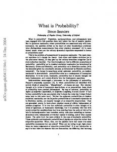
Fig. 3. Examples of a contour set that consists of 13 contour regions: the ascending contour regions p, a1–a4, b1, and b2 and the descending contour regions (with hachured borders, the hachures pointing in the direction of the descent) b3–b5 and c1–c3. Some contour lines are labeled with their boundary values while others are implied because this map is an example of a fixed interval contour set. For example, b1 has a ctrBdV of 200ft, meaning that any point on the boundary of or inside b1, but not inside b2 is guaranteed to have an elevation of at least 200ft and less than 220ft. Equally, points inside b3 but not inside b4 have elevation values not greater than 220ft but greater than 200ft (the implied contour boundary value of b4). This makes clear that not all points in b1 have an elevation above 200ft: the points inside b4 are in fact all below 200ft (this happens, e.g., in a volcanic crater). This 13-element contour set forms a single parent contour set (SPCS ) with p being the root contour region that spatially contains all others. This contour set has many subsets, of which the sets a1–a4, b1–b5, and c1–c3 are all totally ordered contour sets (TOCS ). Among them, a1– a4 is an ascending set (AscTOCS ) and c1–c3 a descending set (DescTOCS ), while b1–b5 is neither. However, b3–b5 is again descending (DescTOCS ).
(CR-T2) ChildCR(x, y, s) ∧ ChildCR(x, z, s) → y = z (each child can have only a single parent) (CR-T3) SiblingCR(x, y, s) → SiblingCR(y, x, s) (the sibling relation is symmetric in the first two parameters) (CR-T4) SiblingCR(x, y, s) → ¬P O(x, y) (sibling contour regions cannot spatially overlap; follows from CS-A4, ChildCR-D, and SiblingCR-D) 2.5
Ascending and Descending Contour Regions
Contour regions come in two variants: either the contour boundary value (and thus the enclosing contour line) denotes the minimal or the maximal contour value for the bounded contour region. This means either all points inside the contour region and not inside any nested contour region have a measured quantity (of the same measured quality as the contour boundary value) that is above (or equal) or below (or equal) to the contour boundary value. As extreme cases, the measured quality could be constant and equivalent to the contour boundary value at all points in the contour region. By convention, contour lines in topographic maps that denote a minimal contour value (indicating a hill) are displayed as regular (non-hachured) lines, while those that denote a maximal contour value (indicating a depression) have dashes (hachures) pointing inwards as shown for b3–b5 and c1–c3 in Figure 39 . Two disjoint and jointly exhaustive subclasses of CR(x) are introduced to formalize this distinction: ascending 9
Other conventions about label direction and positioning are also commonly used.
contour regions, AscCR(x), denoting a contour region with an ascent towards the inside (CR-A1), and descending contour regions, DescCR(x), denoting a contour region with a descent towards the inside (CR-A2). Note that we can only make claims above the points inside the contour region that are not also within any smaller nested contour region because the next contained contour region may be of opposite nature. For example, all points in region b2 − b3 are above 220 feet in elevation, but some points in b2, namely those in b3, are below 220 feet in elevation. CR-A1 and CR-A2 merely impose necessary conditions for contour regions being called ascending or descending, they do not suffice to infer that AscCR and DescCR are exhaustive and disjoint subclasses of CR. Rather, this is imposed by our knowledge about contour semantics, which we must explicitly postulate (CR-A3). Furthermore, because AscCR and DescCR theoretically both permit that all contained points have measured quantities equivalent to their boundary values, we also have to explicitly postulate their disjointness (CR-A4). � (CR-A1) AscCR(x) → ∀s, vx , p, vp inCS (x, s) ∧ ctrBdV (x, vx ) ∧ Point(p) ∧ Cont(p, x) ∧ pointMQ(p, vp ) ∧ mQuality(vp ) � = mQuality(vx ) ∧ ∀y[inCS (y, s) ∧ Cont(p, y) → Cont(x, y)] → vp ≥ vx (an ascending contour region x is a contour region such that every point that is contained in x but not contained in some smaller contour region has a measured quantity greater or equal to the contour boundary value of x) � (CR-A2) DescCR(x) → ∀s, vx , p, vp inCS (x, s) ∧ ctrBdV (x, vx ) ∧ Point(p) ∧ Cont(p, x)∧pointMQ(p, vp )∧mQuality(v p ) = mQuality(vx )∧∀y[inCS (y, s)∧ � Cont(p, y) → Cont(x, y)] → vp ≤ vx (a descending contour region x is a contour region such that every point that is contained in x but not contained in some smaller contour region has a measured quantity less or equal to the contour boundary value of x) (CR-A3) CR(x) → AscCR(x) ∨ DescCR(x) (all contour regions are either ascending or descending) (CR-A4) ¬AscCR(x) ∨ ¬DescCR(x) (ascending and descending contour regions are disjoint) The axioms CR-A5–CR-A8 formalize the relationships between the contour values of a child and a parent in all four combinations of ascending and descending contour regions. This restricts the contour values of the involved contour regions, but not the measured quantities at points inside the contour regions. While contour regions of the same type must have strictly increasing/decreasing contour boundary values (CR-A5, CR-A6), this is not necessarily true for contour regions of opposite types. For example, in Fig. 3 the ascending region b2 and its descending child b3 have the same contour value. This is permissible because the points in between can vary in between 220ft and 240ft (assuming a fixed interval of 20ft), while the descending contour value of 220ft indicates that further inside all point measures dip below 220ft. This is reflected in CRA7 (for a descending child in an ascending parent) and CR-A8 (for an ascending child in a descending parent) . Moreover, any two siblings of the same kind must have identical contour values (CR-A9). By CR-A5 and CR-A6, a child with the same ctrBdV as its parent must be of the opposite type as the parent (CR-T5).
(CR-A5) AscCR(x) ∧ AscCR(y) ∧ ChildCR(x, y, s) ∧ ctrBdV (x, vx ) ∧ ctrBdV (y, vy ) → vx > vy (an ascending contour region x that is a child of another ascending contour region y in s has a higher contour value than y) (CR-A6) DescCR(x) ∧ DescCR(y) ∧ ChildCR(x, y, s) ∧ ctrBdV (x, vx ) ∧ ctrBdV (y, vy ) → vx < vy (a descending contour region x that is a child of another descending contour region y in s has a higher contour value than y) (CR-A7) DescCR(x) ∧ AscCR(y) ∧ ChildCR(x, y, s) ∧ ctrBdV (x, vx ) ∧ ctrBdV (y, vy ) → vx ≥ vy (a descending contour region x that is a child of a ascending contour region y in s has a higher or equal contour value as y) (CR-A8) AscCR(x) ∧ DescCR(y) ∧ ChildCR(x, y, s) ∧ ctrBdV (x, vx ) ∧ ctrBdV (y, vy ) → vx ≤ vy (an ascending contour region x that is a child of a descending contour region y in s has a lower or equal contour value� as y) (CR-A9) SiblingCR(x, y, s) ∧ ctrBdV (x, vx�) ∧ ctrBdV (y, vy ) ∧ [AscCR(x) ∧ AscCR(y)] ∨ [DescCR(x) ∧ DescCR(y)] → vx = vy (sibling contour regions of the same kind must have identical contour values) (CR-T5) ChildCR(x, y, s) ∧ ctrBdV (x, vx ) ∧ ctrBdV (y, vy ) ∧ vx = vy → [AscCR(x) ∧ DescCR(y)] ∨ [DescCR(x) ∧ AscCR(y)] (a child contour region with the same measured quantity as its parent is of the opposite type as its parent) While CV-A6 already postulated that each point on the boundary of a contour region must have a point measure equivalent to the contour boundary value, we can now be more precise: any childless ascending (descending) contour region contains only measured point values higher (lower) than the contour boundary value (CV-A9). For nested contour regions of the same type, point measure inside a parent region but not inside any of its children have a measured value in between the contour boundary values of the parent and the children (CV-A10). Use Fig. 3 as example: all points in p that are not in either of a1, b1, or c1 have a value between 180ft and 200ft. This would be the case even if c1 had a boundary value of 180ft. (CV-A9) inCS (x, s) ∧ ∀y[¬ChildCR(y, x, s)] ∧ ctrBdV (x, vx ) ∧ Point(p) ∧ Cont(p, x) ∧ pointMQ(p, vp ) ∧ mQuality(vx ) � = mQuality(vp ) � → [AscCR(x) → vp ≥ vx ] ∧ [DescCR(x) → vp ≤ vx ] (a childless ascending (descending) CR x contains only points whose values of the same measured quality are higher (lower) or equal to x’s contour boundary value) (CV-A10) ChildCR(x, y, s) ∧ ctrBdV (x, vx ) ∧ ctrBdV (y, vy ) ∧ Point(p) ∧ Cont(p, y) ∧ pointMQ(p, vp ) ∧ ∀z[ChildCR(z, y, s) → ¬Cont(p, z)] ∧ � mQuality(vp ) = mQuality(vz ) → [AscCR(x)� ∧ AscCR(y) → vy ≤ vp < vx ] ∧ [DescCR(x) ∧ DescCR(y) → vx < vp ≤ vy ] (any point measure vp of the same quality as the contour boundary value vy that is within the ascending (descending) CR y and not within any of it children z must have value in between vy and the boundary contour value vx of all its ascending (descending) child CR) 2.6
Contour Lines
Next we define a contour line as the boundary of a contour region (CL-D) with its contour value being the contour boundary value of the contour region it encloses (CtrVD). CtrV-D is included for cognitive clarity only and is not needed later on. Just as we
distinguish ascending and descending contour regions, we distinguish the contour lines that bound them. Alluding to geographic intuition, we call the boundary of an ascending contour region a hill contour (HillC-D) and the boundary of a descending contour region a depression contour (DeprC-D). Because ascending and descending contour regions are disjoint and exhaustive subclasses of contour regions, hill and depression contours are also disjoint and exhaustive (CL-T1, CL-T2). (CL-D) Contour (x) ≡ ∃y[CR(y) ∧ x = bd(y)] (a contour line is the boundary of a contour region) (CtrV-D) ctrV (bd(x)) = v ≡ ctrBdV (x, v) (the contour value of a contour line is the contour boundary value of the contour region it encloses) (HillC-D) HillContour (x) ≡ ∃y[AscCR(y) ∧ x = bd(y)] (a hill contour is the boundary of an ascending contour region) (DeprC-D) DepressionContour (x) ≡ ∃y[DescCR(y) ∧ x = bd(y)] (a depression contour is the boundary of a descending contour region) (CL-T1) Contour (x) → HillContour (x) ∨ DepressionContour (x) (every contour is either a hill or a depression contour) (CL-T2) ¬HillContour (x) ∨ ¬DepressionContour (x) (hill and depression contours are disjoint) We can now also formally define adjacency between contours within a contour set. Contours that bound regions that are in a parent-child or in a sibling relation are adjacent, as are contours of two parent-less contour regions – a case that is only possible in contour sets without a single parent. This definition captures the fundamental adjacency relation between contour lines used in the contour data structures developed in [6]. h (AdjCL-D) AdjacentContours(m, n) ≡ ∃s, x, y m = bd(x) ∧ n = bd(y) ∧ � inCS (x, s) ∧ inCS (y, s) ∧ ChildCR(x, y, s) ∨ SiblingCR(x, y, s) ∨ �i ∀z[inCS (z, s) → (x = z ∨ ¬Cont(x, z)) ∧ (y = z ∨ ¬Cont(y, z))] (two contour lines are adjacent iff they bound contour regions x and y in a common contour set s such that they are either in a parent-child relation, in a sibling relation, or any other contour region in s properly contains neither x nor y)
3
More Specialized Contour Sets
So far, the class GenCS denotes arbitrary sets of contour regions whose contour values are about a common measured quality without further restrictions on acceptable contour values, their spatial configuration, or the presence/absence of ascending or descending contour regions. Next we will refine this generic class to more interesting and more narrowly defined subclass as shown in the hierarchy of contour sets in Figure 4. 3.1
Fixed (Constant) Interval Contour Sets (FICS )
Most contour maps that display terrain information have a constant interval between adjacent contours. For example, the National Map commonly uses 20 feet contour intervals, but also intervals of 5, 10, 40, or 50 feet. That means all contour regions within a single contour set have only contour boundary values that are a multiple of 20 (or 5, 10, 40 or 50) feet. We capture this idea in the class of fixed interval contour sets,
Fig. 4. The hierarchy of classes of contour sets. The class FICS uses the existence of a constant interval between contours as distinguishing criterion, which is independent of the criteria used for distinguishing the classes SPCS , TOCS , AscTOCS , and DescTOCS from GenCS . Thus, the class FICS is not necessarily disjoint with any of the other classes of contour sets.
FICS . Each fixed interval contour set has a unique contour interval defined (FICS-D, FICS-A1) as indicated by the relation ctrInterval (s, i) between a contour set s and its contour interval i. Conversely, the existence of a contour interval suffices to ensure that a contour set s is a fixed interval contour set – a property that helps express subsequent axioms and theorems more succinctly. FICS-A2 captures the essential condition of what it means for a contour set to have a fixed interval: the difference between any two contour boundary values in the set is equivalent to baseValue + k · contourInterval for some integer k and constant values baseValue and contourInterval. This applies to sets of contours that are all multiples of a contour interval, but also accommodates the more general case of sets of contours with constant intervals yet unusual base values (e.g. contours at 5, 25, 45, and 65 feet). Within our formalization there is no need to fix the base value – in fact, it is never explicitly mentioned. Finally, fixed interval contour sets require that the measured property uses at least an interval scale (FICS-A3), otherwise the contour interval lacks clear semantics. (FICS-D) FICS (s) → GenCS (s) ∧ ∃i[ctrInterval (s, i)] (each fixed interval contour set is a contour set that has a contour interval) (FICS-A1) ctrInterval (s, i) ∧ ctrInterval (s, j) → i = j (each contour set has at most one contour interval; it is a functional attribute) (FICS-A2) ctrInterval (s, i) ∧ inCS (x, s) ∧ inCS (y, s) ∧ ctrBdV (x, vx ) ∧ ctrBdV (y, vy ) → ∃k[Integer(k) ∧ vx = vy + k · i] (the difference between the contour boundary values of any two contour regions in a fixed interval contour set is a multiple of the set’s contour interval) (FICS-A3) ctrInterval (s, i) → FICS (s) ∧ MQuantity(i) ∧ ∃x[mScale(i, x) ∧ IntervalMScale(x)] (ctrInterval (s, i) denotes that the contour set s has a fixed measured quantity i as its contour interval with an interval scale associated to it) (FICS-A4) ctrInterval (s, i) ∧ ChildCR(x, y, s) ∧ ctrBdV (x, vx ) ∧ ctrBdV (y, vy ) → (x − y = i ∨ y − x = i ∨ x − y = 0) (the absolute difference between a parent and a child contour region in a fixed interval contour set is either the contour interval or 0) Now the additional properties FICS-T1–FICS-T5 about the contour boundary values of parents, children, and siblings in a fixed interval contour set become provable.
(FICS-T1) ctrInterval (s, i) ∧ ChildCR(x, y, s) ∧ ctrBdV (x, vx ) ∧ ctrBdV (y, vy ) ∧ AscCR(x) ∧ AscCR(y) → vx − vy = i (in a fixed interval contour set, the difference between the boundary values of an ascending child contour region and its ascending parent is the contour interval) (FICS-T2) ctrInterval (s, i) ∧ ChildCR(x, y, s) ∧ ctrBdV (x, vx ) ∧ ctrBdV (y, vy ) ∧ DescCR(x) ∧ DescCR(y) → vy − vx = i (in a fixed interval contour set, the difference between the boundary values of a descending parent contour region and its descending child is the contour interval) (FICS-T3) FICS (s) ∧ SiblingCR(x, y, s) ∧ ctrBdV (x, vx ) ∧ ctrBdV (y, vy ) ∧ AscCR(x) ∧ AscCR(y) → vx = vy (ascending sibling contour regions in a fixed interval contour set have equivalent contour boundary values) (FICS-T4) FICS (s) ∧ SiblingCR(x, y, s) ∧ ctrBdV (x, vx ) ∧ ctrBdV (y, vy ) ∧ DescCR(x) ∧ DescCR(y)∧ → vx = vy (descending sibling contour regions in a fixed interval contour have equivalent contour boundary values) (FICS-T5) ctrInterval (s, i) ∧ inCS (x, s) ∧ inCS (y, s) ∧ ctrBdV (x, vx ) ∧ ctrBdV (y, vy ) ∧ Integer(k) ∧ vx < ki < vy → ∃z[∧inCS (z, s) ∧ ctrBdV (z, ki)] (for any multiple k of a contour set’s contour interval i, if ki is between the boundary contour values vx and vy of contour regions x and y in s, then some contour region z in s has ki as contour boundary value) Mathematical Characterization of GenCS and FICS The contour regions within a generic contour set and their spatial containment relation exhibit mathematically welldefined structures in all models of the ontology of generic contour maps GCtrMap = {CR-A1–CR-A9, CV-A1–CV-A10, CS-A1–CS-A6, CRChild-D, CRSibling-D}10 . Each model forms a forest – a set of trees – as formalized by the following theorem. The superscript notation P M denotes the interpretation of predicate P under the model M. Theorem 1. Let M be an arbitrary model of the ontology GCtrMap. For each S ∈ GenCS M , let (x, y) ∈ Cont ⇔ (x, S), (y, S) ∈ inCS M and (x, y) ∈ Cont M . Then (S, Cont) is a forest. Proof (Sketch). Recall that any two contour regions in a common contour set are either in a spatial containment relation or do not overlap at all (CS-A3). If two contour regions are in a spatial containment relation, they form a parent-child relation in the tree. By CR-T2, each child has at most one parent and Cont is antisymmetric (see [7]), hence no cycles exist. Thus, each parent-less contour region in S forms a tree. Because (S, Cont) can contain multiple parent-less contour regions, it is a forest. t u A consequence of this theorem is that the underlying field of a contour set is covered by the spatial extent of all its parent-less (root) contour regions. Each spatial location of the underlying field is thus in exactly one of the root contour regions. This theorem extends to the structures (S, Cont) defined over instances of FICS , which are also forests. The only difference is that in fixed interval contour sets the interval between the contour boundary values of a parent and its children in the tree is constrained. In the next section, we will look at other types of contour sets that further constrain the underlying mathematical structure over the spatial containment relation. 10
For brevity, this ontology excludes all definitions that are unnecessary for the characterization.
3.2
Totally Ordered Contour Sets (TOCS )
Generic and fixed interval contour sets do not have a single root contour region as just shown by the mathematical characterization. Now we specifically define a class of contour sets – the single parent contour sets denoted as SPCS (s) – that have a unique contour region that spatially contains all other contour regions in the set (SPCS-D). This region serves as the root of the contour set. Note that the two subclasses of generic contour sets, the single parent contour sets SPCS and the fixed interval contour sets FICS , are not necessarily disjoint and neither is a subclass of the other. As further specializations of single parent contour sets, we call a single parent contour set s a totally ordered contour set, TOCS (s), if, and only if, no contour region therein has a sibling. We distinguish two subclasses of totally ordered contour sets: ascending totally ordered contour sets, AscTOCS (s), and descending totally ordered contour sets, DescTOCS (s). These two classes capture specific geographic phenomenon – hills and depressions – of particular interest to elevation contours as displayed on topographic maps. For example, in Fig. 3 the contour set consisting of a1–a4 is an ascending totally ordered contour set that describes a hill, while the two contour sets consisting of b3–b5 and c1–c3, respectively, form descending totally ordered contour sets that describe depressions (mine holes in this case). (SPCS-D) SPCS (s) ≡ GenCS (s) ∧ ∃x[inCS (x, s) ∧ ∀y[inCS (y, s) → Cont(y, x)]] (A single parent contour set has a unique largest contour region that spatially contains all other contour regions in the set) (TOCS-D) TOCS (s) ≡ SPCS (s) ∧ ¬∃x, y[SiblingCR(x, y, s)] (a totally ordered contour set is a SPCS that does not contain any siblings) (AscTOCS-D) AscTOCS (s) ≡ TOCS (s) ∧ ∀x[inCS (x, s) → AscCR(x)] (an ascending TOCS is a TOCS that consists only of ascending contour regions) (DescTOCS-D) DescTOCS (s) ≡ TOCS (s) ∧ ∀x[inCS (x, s) → DescCR(x)] (an descending TOCS is a TOCS that consists only of descending contour regions) (TOCS-T1) TOCS (s) ∧ ChildCR(x, z, s) ∧ ChildCR(y, z, s) → x = y (each contour region z in a TOCS contains no more than one child) (TOCS-T2) AscTOCS (s) ∧ ChildCR(x, y, s) ∧ ctrBdV (x, vx ) ∧ ctrBdV (y, vy ) → vx > vy (boundary values in an ascending TOCS increase towards the inside) (TOCS-T3) DescTOCS (s) ∧ ChildCR(x, y, s) ∧ ctrBdV (x, vx ) ∧ ctrBdV (y, vy ) → vx < vy (boundary values in a descending TOCS decrease towards the inside) Mathematical Characterization of TOCS , AscTOCS , and DescTOCS Now, we can extend Theorem 1 to characterize the substructures (S, Cont) formed by contour sets that are (ascending/descending) totally ordered contour sets in models of the ontology TOCtrMap = GCtrMap ∪ {SPCS-D, TOCS-D, AscTOCS-D, DescTocs-D}. This new ontology TOCtrMap is a definitional extension of GCtrMap. Theorem 2. Let M be an arbitrary model of the ontology TOCtrMap. For each S ∈ GenCS M , let (x, y) ∈ Cont ⇔ (x, S), (y, S) ∈ inCS M and (x, y) ∈ Cont M . If S ∈ SPCS M , then (S, Cont) is a tree. If S ∈ TOCS M , then (S, Cont) is a chain. Proof (Sketch). Each so-defined structure (S, Cont) is a forest by Theorem 1. Now suppose S ∈ SPCS M . Then by SPCS-D, S has a unique root and thus is single-
rooted and, thereby, connected. But every connected forest is a tree. Now suppose S ∈ TOCS M . Then by TOCS-D each parent has at most one child. Because each contour region has at most one parent (CR-T2), it follows that spatial containment totally orders the tree’s contour regions such that the tree is a chain. t u This characterization of every instance of SPCS forming a tree over the spatial containment relation matches the description of each contour line forming an enclosure tree over its nested contours lines given by [1].
4
Definable Areas of Physical-Geographical Significance
For many purposes, spatial regions that are not contour regions themselves, but that can be defined in terms of them, are of practical interest. These include regions of equal contour value, each of which is a contour region minus the region of all its children. For example, in Fig. 3, the area of p minus the areas of a1, b1, and c3 forms a region of equal contour value with elevations between 180 and 200 feet. Within that area, we cannot distinguish the elevation measure between any two points – it hits the resolution threshold inherent in the chosen contour interval. Such areas are possibly holed and/or disconnected11 . We define this area using the sum and difference operations on regions (CA= -D). By CV-A10, all points in such an ascending (descending) region x have measured quantities between x’s contour boundary value and the minimum (maximum) contour boundary value of all its ascending (descending) children. The definition of cArea = (x, s) for arbitrary regions enables us to define the entire, possibly disconnected subarea of a contour region that is above (below) the contour boundary value of x. To define such area, all contained contour areas with boundary values above (below) that of x are summed up (CA> -D, CA< -D). To make these definitions more palatable, we first define a subset of all contour regions in s that are contained in x and have at least (at most) the contour boundary value of x (GCS> -D and GCS< -D). It immediately follows that within an ascending (descending) totally ordered contour set, the spatial extent of any contour region is equivalent to its contour area cArea > (cArea < ) (CA> -T1, CA< -T1). (CA= -D) inCS (x, s) → cArea = (x, s) = x − Σ(y|ChildCR(y,x,s)) y (the contour area of equal value, cArea = (x, s), of contour region x in s is the area of x minus the area of all its children) (GCS> -D) GenCS > (t, s, x) ≡ ∀y[inCS (y, t) ↔ inCS (y, s) ∧ Cont(y, x) ∧ ctrBdV (x, vx ) ∧ ctrBdV (y, vy ) ∧ vy ≥ vx ] (t is the subset of s’s contour regions that are spatially contained in x and have a boundary value no smaller than x) (CA> -D) cArea > (x, s) = Σ(y|inCS (y,t)∧GenCS > (t,s,x)) cArea = (y, s) (the area within x with measured values above the contour boundary value of x) (GCS< -D) GenCS < (t, s, x) ≡ ∀y[inCS (y, t) ↔ inCS (y, s) ∧ Cont(y, x) ∧ ctrBdV (x, vx ) ∧ ctrBdV (y, vy ) ∧ vy ≤ vx ] (t is the subset of s’s contour regions that are spatially contained in x and have a boundary value no bigger than x) 11
The region of equal contour value is only disconnected when separated by two or more cliffs, which are points/segments of its containing contour region where it shares a portion of its boundary with one or multiple child contour regions.
(CA< -D) cArea < (x, s) = Σ(y|inCS (y,t)∧GenCS < (t,s,x)) cArea = (y, s) (the area within x with measured values above the contour boundary value of x) (CA> -T1) AscTOCS (s) ∧ inCS (x, s) → cArea > (x, s) = x (each contour region in a ascending TOCS has itself as ascending contour area) (CA< -T1) DescTOCS (s) ∧ inCS (x, s) → cArea < (x, s) = x (each contour region in a descending TOCS has itself as descending contour area) The areas cArea > (x, s) and cArea < (x, y) can be visualized as the areas that are included (or excluded) when the surface defined by the underlying field is intersected with a horizontal plane at the elevation of x’s boundary. These areas are geographically significant in many applications. For example, on elevation contour maps the area cArea < (x, s) indicates the portion of the landscape that is submerged in a lake with a certain water level as indicated by x as the lake boundary. Equally, a certain elevation threshold may be used to identify areas prone to flooding because of their elevation below a certain threshold expressed as a contour region with suitable contour boundary value. The areas above the threshold that are completely surrounded by lower-lying areas will become “islands” in the case of flooding. The areas cArea > (x, s) and cArea < (x, y) can also be used to identify vegetation or habitat zones defined by a certain elevation threshold.
5
Discussions and Conclusions
In this paper, we formally analyzed the inherent, yet implicit semantics of contour maps and axiomatized it as a rigorous first-order ontology amendable to automated reasoning as necessary for achieving computational spatial intelligence. While humans adhere to the implicit semantics buried in contour maps without difficulties, the explicit axiomatization is a necessary first step towards employing contour information directly for fully automated reasoning by general purpose reasoners (such as theorem provers), which can answer broader ranges of queries as compared to the highly customized spatial algorithms that are currently used in geographic information systems. The resulting ontology is largely based on the purely qualitative representation of space from [7] that relies exclusively on mereotopological (of contact and parthood) relations among abstract spatial regions of different dimensions such as points, curves (here specifically simple loop curves), areal regions, and associated spatial relations defined in terms of spatial containment (the subregion relation). The ontology adapts the ontology pattern from [20] about measured quantities to specify how contours and contour regions within a contour map are associated with a shared measured quality, such as elevation, and how the values on contour lines are related to point measures inside the regions they bound. Besides the imported spatial concepts and relations, the formalization requires very few additional primitive concepts and relations: contour regions CR, its subclasses AscCR and DescCR and its associated relation ctrBdV as well as primitives to specify sets of contour regions (contour sets GenCS and the related membership relation inCS ). Foundation for Quantitatively Enhanced Qualitative Spatial Reasoning Purely qualitative representations of space [2, 3, 7, 9] can answer only the simplest common sense questions about space. In many cases, such representations must be supplemented
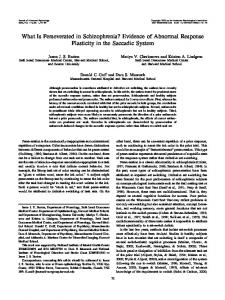
Fig. 5. The manually derived conceptual model of conceptual contour maps in UML notation based on the first-order ontology. This simplified model excludes concepts and relations pertaining to the various defined areas from Sec. 4 and is limited to fixed interval contour sets. It introduces new concepts ParentChildContours and SiblingContours (displayed with dashed borders) that result from encoding the ternary relations ChildCR and SiblingCR using binary ones. While the conceptual model provides a visual summary of the ontology, it is no adequate replacement. Many of the intricate relationships in contour maps, such as between contour regions and their contour values within a contour set, are not at all visible in the conceptual model.
by simple quantitative reasoning, as exemplified by the presented formalization, which through the use of simple quantitative operations greatly increases the utility of a predominantly qualitative representation of space. In this spirit, the presented formalization lays the foundation for automated contour-based spatial reasoning by not only providing a set of axioms that explicitly captures the semantics of contour maps, but also through the identification of the quantitative operations necessary to support reasoning about them. This contour-based spatial reasoning takes conventional qualitative, region-based reasoning formalisms such as the RCC [19] or CODIB [7, 8] to the next level by integrating it with quantitative information – the measures/observations – at locations within such spatial regions. Our ontology show that simple integer operations (sum, difference, multiplication, and (in)equalities) for contour values and a spatial sum operation (Σ) over sets of spatial regions suffice to support qualitative-quantitative reasoning about contours. That means a computational framework for reasoning about contours can rely primarily on non-quantitative mereotopological reasoning (similar to reasoning with the Region Connection Calculus [19]) if complemented by a quantitative reasoner that can efficiently perform basic integer operations and calculate sums of spatial regions. We anticipate that such hybrid qualitative-quantitative reasoning can
answer simple, common sense geographical queries as exemplified in Sec. 1.1, such as identifying the elevation profile of a path, comparing regions with respect to their max/min elevation or roughness, estimating volumes of depressions, waterbodies and reservoirs, or identifying the extent of areas prone to flooding, without having to employ a full quantitative model of a field as currently done in geographic information systems build on data types and algorithms from computational geometry. Derived Conceptual Model While the intricate interplay between qualitative and quantitative constraints in contour maps justifies the use of first-order logic for our detailed ontological analysis, the developed ontology is not necessarily ideal for storing and querying information of particular contour maps. Thus, a translation of the ontology into a less expressive, yet still computer-interpretable language (e.g., from the OWL family) will foster broader adoption and reuse. While such extraction could be largely automated, certain first-order logical constructs must be remodeled to adapt to the restrictions that less expressive languages impose. For example, the ternary relations ChildCR, SiblingCR, GenCS > , and GenCS < need to be split into new concepts and associated sets of binary relations in order to represent them in OWL. The portion of the semantics that can be expressed in, e.g., OWL Full and the constraints that would be lost in such a representation remain to be investigated. As a step towards fostering broader use, we manually derived the simplified conceptual model shown in Fig. 5 that relates the key contour concepts: contour regions, contour lines, contour values, and contour sets. It further distinguishes between ascending (shown in brown) and descending (in blue) contour regions, lines, and sets. While AscCR and DescCR, and HillContour and DepressionContour exhaustively classify contour regions and lines, respectively, AscTOCS and DescTOCS are non-exhaustive special cases of contour sets. To improve readability, the full classification of contour sets from Fig. 4 has been omitted from Fig. 5, focusing instead on contours with fixed contour intervals, which are prevalent in many applications, including topographic maps. Relationship to Surface Water Networks We have justified many contour-related concepts using simple physical-geographical features that we would like to locate on topographic contour maps, such as hills, peaks, depressions, pits, saddles, and cliffs. However, many more geographical features, in particular those that play a central role in surface networks [21] and surface water networks [14, 22], can be more accurately spatially grounded in elevation contour maps. This requires a fuller investigation of how surface water features, including channels, pour points, and watershed basins, are related to the identified concepts on contour maps. Acknowledgments Part of this paper is based on discussions about key concepts in contour maps at the joint SOCoP (Spatial Ontology Community of Practice) and GeoVoCamp workshop in Madison, WI in June 2014, continued at a GeoVoCamp meeting at USGS in Reston, VA in December 2014. We gratefully acknowledge and thank those who contributed to these preliminary discussions: Carl Sack (at Madison), Joshua Lieberman, Dave Kolas and John (Ebo) David (at Reston), and in particular Dalia Varanka for her valuable contributions at both workshops. We further thank the workshop organizers Nancy Wiegand and Gary Berg-Cross, whose efforts to organize these events enabled those fruitful discussions. Finally, we appreciate the constructive comments of Philip Thiem and four anonymous reviewers, which helped improve the final paper.
References 1. Boyell, R., Ruston, H.: Hybrid techniques for real-time radar simulation. In: IEEE Fall Joint Computer Conference (IEEE 1963). (1963) 445–458 2. Casati, R., Varzi, A.C.: Parts and Places. MIT Press (1999) 3. Cohn, A.G., Renz, J.: Qualitative Spatial Representation and Reasoning. In van Harmelen, F., Lifschitz, V., Porter, B., eds.: Handbook of Knowledge Representation. Elsevier (2008) 4. Egenhofer, M.J., Mark, D.M.: Naive Geography. In: Conf. on Spatial Inf. Theory (COSIT95). LNCS 988, Springer (1995) 1–15 5. Egenhofer, M.J., Sharma, J.: Topological relations between regions in R2 and Z 2 . In: Symp. on Large Spatial Databases (SSD’93). LNCS 692, Springer (1993) 316–336 6. Freeman, H., Morse, S.: On searching a contour map for a given terrain elevation profile. J. Franklin Institute 284(1) (1967) 1–25 7. Hahmann, T.: A Reconciliation of Logical Representations of Space: from Multidimensional Mereotopology to Geometry. PhD thesis, Univ. of Toronto, Dept. of Comp. Science (2013) 8. Hahmann, T., Grüninger, M.: A naïve theory of dimension for qualitative spatial relations. In: Symp. on Logical Formalizations of Commonsense Reasoning (CommonSense 2011), AAAI Press (2011) 9. Hahmann, T., Grüninger, M.: Region-based Theories of Space: Mereotopology and Beyond. In Hazarika, S.M., ed.: Qualitative Spatio-Temporal Representation and Reasoning: Trends and Future Directions. IGI (2012) 1–62 10. Hutton, C.: An account of the calculations made from the survey and measures taken at schehallien. Philosophical Transactions of the Royal Society of London 68 (1778) 11. Kweon, I., Kanade, T.: Extracting topographic terrain features from elevation maps. CVGIP: Image Understanding 59 (1994) 171–182 12. Masolo, C., Borgo, S., Gangemi, A., Guarino, N., Oltramari, A.: Wonderweb deliverable D18 - ontology library (final report). Technical report, National Research Council - Institute of Cognitive Sci. and Technology, Trento (2003) 13. Morse, S.: Concepts of use in contour map processing. Comm. ACM 12 (1969) 147–152 14. O’Callaghan, J., Mark, D.M.: The extraction of drainage networks from digital elevation data. Computer vision, graphics, and image processing 28(3) (1984) 323–344 15. Open Geospatial Consortium (OGC): OGC Reference Model. http://www.opengeospatial.org/standards/orm (12 2011) OGC 08-062r7. 16. Open Geospatial Consortium (OGC): ISO 19156: Geographic information – observations and measurements. http://www.opengeospatial.org/standards/om (09 2013) OGC 10-004r3. 17. Pike, R., Evans, I., Hengle, T.: Geomorphometry: A brief guide. In Hengl, T., Reuter, H., eds.: Geomorphometry: Concepts, Software, Applications. Elsevier (2009) 18. Rana, S., ed.: Topological Data Structures for Surfaces. Wiley (2004) 19. Randell, D.A., Cui, Z., Cohn, A.G.: A spatial logic based on regions and connection. In: KR’92: Principles of Knowledge Representation and Reasoning. (1992) 165–176 20. Rijgersberg, H., van Assem, M., Top, J.: Ontology of units of measure and related concepts. Semantic Web Journal 4(1) (2013) 3–13 21. Sinha, G., Kolas, D., Mark, D., Romero, B.E., Usery, L.E., Berg-Cross, G., Padmanabhan, A.: Surface network ontology design patterns for linked topographic data. (May 2014) 22. Sinha, G., Mark, D., Kolas, D., Varanka, D., Romero, B.E., Feng, C.C., Usery, L.E., Liebermann, J., Sorokine, A.: An ontology design pattern for surface water features. In: 8th Int. Conf. on Geographic Information Science (GIScience 2014). (2014) 23. Stevens, S.S.: On the Theory of Scales of Measurement. Sci. 103(2684) (1946) 677–680 24. Usery, E.L., Varanka, D., Finn, M.P.: A 125 year history of topographic mapping and GIS in the U.S. Geological Survey 1884-2009, Part 1, 1884-1980 (March 2015)