Windows Scheduling of Arbitrary Length Jobs on ... - Semantic Scholar

Windows Scheduling of Arbitrary Length Jobs on Parallel Machines Amotz Bar-Noy∗

Richard E. Ladner†

Tami Tamir ‡

Tammy VanDeGrift§

ABSTRACT

1.

The generalized windows scheduling problem for n jobs on multiple machines is defined as follows: Given is a sequence, I = h(w1 , `1 ), (w2 , `2 ), . . . , (wn , `n )i of n pairs of positive integers that are associated with the jobs 1, 2, . . . , n, respectively. The processing length of job i is `i slots (a slot is the processing time of one length unit). The goal is to repeatedly and non-preemptively schedule all the jobs on the fewest possible parallel machines such that the gap (window) between two consecutive executions of the first slot of job i is at most wi slots. This problem arises in push broadcast systems in which data is transmitted on parallel channels. The problem is NP-hard even for unit-length jobs and a (1+ε)-approximation algorithm is known for this Pcase by approximating the natural lower bound W (I) = n i=1 (1/wi ). The techniques used for approximating unit-length jobs cannot be applied for arbitrary-length jobs mainly because the optimal number of machines might be arbitrarily larger than Pn the generalized lower bound W (I) = i=1 (`i /wi ). Our main result is an 8-approximation algorithm for the generalized windows scheduling problem using new methods, different from those used for the unit-length case. We also present an algorithm that uses 2(1 + ε)W (I) + log wmax machines and a greedy algorithm that is based on a new tree representation of schedules. The greedy algorithm is optimal for some special and simulations show that it performs very well in practice.

The generalized windows scheduling problem for n jobs on parallel machines is defined as follows: Given is a sequence of n positive integer pairs I = h(w1 , `1 ), (w2 , `2 ), . . . , (wn , `n )i that are associated with the jobs 1, 2, . . . , n, respectively. The processing length of job i is `i slots. For simplicity, we assume integer lengths and that each unit of length takes one slot of time in the schedule. The goal is to repeatedly and non-preemptively schedule all the jobs on the fewest possible parallel machines such that the gap (window) between any two consecutive executions of the first slot of job i is at most wi slots.

∗

Computer & Information Science Department, Brooklyn College, 2900 Bedford Ave., Brooklyn, NY 11210. [email protected] † Department of Computer Science and Engineering, Box 352350, University of Washington, Seattle, WA 98195. [email protected]. Research partially supported by NSF grant CCR-0098012. ‡ School of Computer Science, The Interdisciplinary Center, Herzliya, Israel. [email protected] § Electrical Engineering & Computer Science, University of Portland, 5000 N. Willamette Blvd., Portland, OR 97203. [email protected]

Permission to make digital or hard copies of all or part of this work for personal or classroom use is granted without fee provided that copies are not made or distributed for profit or commercial advantage and that copies bear this notice and the full citation on the first page. To copy otherwise, to republish, to post on servers or to redistribute to lists, requires prior specific permission and/or a fee. SPAA’05, July 18–20, 2005, Las Vegas, Nevada, USA. Copyright 2005 ACM 1-58113-986-1/05/0007 ...$5.00.

INTRODUCTION

Example: Let I = h(4, 2), (8, 4), (8, 2), (16, 4), (16, 4)i for jobs a, b, c, d, e, respectively. By calculating the total processing requirements of the jobs, it is clear that more than one machine is needed. A possible schedule using 2 machines is the following: [a, a, c, c, a, a, ∗, ∗] on one machine and [b, b, b, b, d, d, d, d, b, b, b, b, e, e, e, e] on the other. Schedules are represented by their periodic cycle where the “∗” symbol stands for an idle slot. Observe that the window between any two appearances of any of any of the five jobs is always exactly as required. The windows scheduling problem belongs to the class of periodic scheduling problems in which n jobs need to be scheduled infinitely often on m parallel machines (the number of machines is sometimes part of the input and not an optimization goal). Each job has a length and is associated with a frequency (or share) requirement. For example, a job might need to be executed one half of the time. The quality of a periodic schedule is measured by the actual frequencies in which the jobs are scheduled, and the regularity of the schedule regarding the gaps between consecutive executions of each job. This distinguishes periodic scheduling from traditional scheduling in which each job is executed only once and is associated with parameters like release time and deadline. The traditional optimization goal for periodic scheduling is an “average” type goal in which job i must be executed a specific fraction of the time. Our problem considers a different objective of a “max” type: the gap between any two consecutive executions of job i must be at most wi which implies in particular that job i is executed at least `i /wi of the time. Previous results for the windows scheduling problem either assumed one machine with unit-length jobs (the pinwheel problem [21, 22]), unit-length jobs with multiple machines ([4, 6]), or one machine with arbitrary-length jobs (the generalized pinwheel problem [10, 16]). To the best of

our knowledge, we are the first to consider the generalized windows scheduling problem.

1.1

Applications and Motivation

Periodic scheduling in general and windows scheduling in particular can be thought of as a scheduling problem for push broadcast systems (as opposed to pull broadcast systems). One example is the Broadcast Disks environment (e.g., [1]) where satellites broadcast popular information pages to clients. Another example is the TeleText environment (e.g., [2]) where running banners appear in some television networks. In such systems, there are clients and servers where the servers choose what information to push and in what frequency in order to optimize the quality of service for the clients. This optimization objective belongs to the average type periodic scheduling problems. In a more generalized model (e.g., [7, 19]), the servers “sell” their broadcasting service to various providers who supply content and request that the content be broadcast regularly. The regularity can be defined by a window that represents the maximum delay before a client receives a particular content. This is modelled by the windows scheduling problem. In harmonic windows scheduling (e.g., [5]), jobs represent segments of movies. For 1 ≤ i ≤ n, the window of segment i is wi = D + i, where n is the number of equally sized segments of the movie and DL/n is the guaranteed startup delay for an uninterrupted playback of a movie of length L. Harmonic windows scheduling is the basis of many popular media delivery schemes (e.g., [24, 23]) that are based on the concept of receiving data from multiple channels and buffering data for future playback. This concept was first developed in [30] and was the subject of numerous papers in the last decade. There is an interesting application of the generalized windows scheduling problem in compressed video delivery. When the video is compressed, frame (segment) i is associated with a length `i measured in time slots. Different compressed frames may have different lengths. Let L be the length of a decompressed frame also in time slots. The entire frame would have to be received before it could be decompressed and played back. Suppose the desired delay to play back the video is D slots. The first frame of length `1 must be entirely received in every window of size w1 = D. The second frame of length `2 must be entirely received in every window of size w2 = D + L. In general, the ith frame of length `i must be entirely received in every window of size wi = D + (i − 1)L.

1.2

Related Work

The pinwheel problem was defined in [22] and the generalized pinwheel problem was considered in [10, 16]. In these and other papers about the pinwheel problem, the focus was to understand which inputs can be scheduled on one machine. For example, [12] optimized the bound on the P value of n i=1 (1/wi ) that guarantees a feasible schedule [12]. The windows scheduling problem was defined in [4] where schedules were defined that use opt + O(ln(opt)) machines, where opt is the number of machines used by an optimal solution. In [27] periodic scheduling was defined to be a schedule where a job with window w is scheduled exactly once in every time interval of the form [(k − 1)w, kw] for any inte-

ger k. This is a typical fairness requirement for the average type periodic scheduling. In [28] an optimal solution for the chairman assignment problem was presented for a stronger fairness condition that depends on the prefix of the schedule. These papers considered unit-length jobs on a single machine. In the generalized model, each job has an arbitrary length and it can be scheduled on multiple machines. For this case, [9] proposed Pfair schedules in which the number of slots allocated to a job whose share request (measured by the fraction of time it should be processed) is f in any prefix of t time slots is either bf · tc or df · te. The broadcast disks problem, which is an average type periodic scheduling problem, was introduced in [1]. Unitlength jobs were addressed and constant approximation solutions were presented in [3]. These results were improved in [26] which presented a polynomial time approximation scheme. The arbitrary length case was considered and a constant approximation solution was presented in [25]. In perfect periodic schedules, each job has a fixed window size (a period) between consecutive executions. The objective is to minimize the maximum or average ratio between the granted period and the requested one. This problem differs from windows scheduling since jobs may get larger windows than their request. The unit-length case was considered in [8] and the general case of jobs with arbitrary lengths was considered in [11]. Windows scheduling with unit-length jobs is a special case of the bin packing problem (e.g., [13]) and one of our results takes advantage of this fact. In the unit fractions bin packing problem, the goal is to pack all the items in bins of unit size where the size of item i is 1/wi . In a way, bin packing is the fractional version of windows scheduling where windows scheduling imposes another restriction on the packing. The relationship between these two problems and their off-line and the on-line cases were considered in [6]. Recent work on video-on-demand systems has provided lower bounds on delay required to deliver media that also applies to the special case of windows scheduling as a media delivery scheme [14, 15, 20]. These bounds can be achieved in the limit in the windows scheduling model [5].

1.3

Contributions

Notations and definitions: Denote by w-job a job with window w and by (w, `)-job a job with window w and length `. An instance in which all the windows and all the lengths are powers of 2 is called a P power-2 instance. The width of a (w, `)-job is `/w. W (I) = n i=1 (`i /wi ) is the total width of the jobs in I = h(w1 , `1 ), (w2 , `2 ), . . . , (wn , `n )i. We consider only non-preemptive schedules in which the `i slots allocated to job i must be successive. We note informally that the preemptive version is identical to windows scheduling of unitlength jobs by replacing each (w, `)-job by ` (w, 1)-jobs. We assume that `i ≤ wi for all 1 ≤ i ≤ n. Otherwise, the definition of schedules and windows should be modified. Two special types of schedules are Perfect schedules – in which for each job there exists some wi0 ≤ wi such that the gap between any two executions of job i is exactly wi0 slots, and Thrift schedules – that are perfect schedules in which for all i, wi0 = wi . For an instance I, let OP T (I) denote the number of machines used in an optimal, not necessarily thrift, schedule, and let OP TT (I) denote the number of machines

used in an optimal thrift schedule. Since a restricted version of the optimal windows scheduling problem is NP-hard even for one channel ([3, 16, 6]), we look for approximate solutions. A natural lower bound to the generalized windows scheduling problem is the total width of the jobs. Since job i requires P at least `i /wi fraction of a machine, at least W (I) = n i=1 (`i /wi ) machines are required in order to accommodate all the jobs. For the unit-length case this lower bound is very close to the optimal solution and indeed (1+ε)-approximation solutions exist for small values of ε. The following example demonstrates that this lower bound can be arbitrarily far from the optimal solution for the generalized windows scheduling problem. Example: Let I = h(r, 1), (r2 , r), . . . , (rn , rn−1 )i be an instance consisting of n jobs where r ≥ 2 is an integer. It is not hard to see that no two jobs can be executed on the same machine and therefore any feasible schedule must use at least n machines. On the other hand, each job demands 1/r of a machine for a total demand of n/r machines. Thus, the ratio between the optimal solution and this lower bound is at least r which can be arbitrarily large. We develop new approximation algorithms that are based on novel methods and techniques. We consider two special cases: (i) In thrift schedules the gap between two executions of job i must be exactly wi (in non-thrift schedules jobs may be scheduled more frequently). (ii) In power-2 instances, windows and lengths are powers of 2. This case can be optimally solved for unit-length jobs, but complex and interesting problems arise in the general case. In particular, the thriftiness paradox presented in this paper implies that even for power-2 instances it might be useful to schedule some jobs more frequently than their demand in order to use fewest machines. For thrift schedules of power-2 instances, we present an optimal algorithm. This algorithm serves as the basis for an 8-approximation algorithm for the generalized windows scheduling problem after rounding both the windows and the lengths to power of 2 values. We also present an algorithm that uses 2(1 + ε)W (I) + log wmax machines and a greedy algorithm that is based on a tree representation of schedules. This greedy algorithm is evaluated by simulation, and performs very well in practice. A variant of this algorithm is optimal for thrift schedules of power-2 instances.

2.

PRELIMINARIES

2.1

Hardness Proof

P B/4 < s(x) < B/2 and such that x∈A s(x) = B. Output: Is there a partition of A intoPm disjoint sets, S1 , S2 , . . . , Sm , such that, for 1 ≤ i ≤ m, x∈Si s(x) = B? (Note that the above constraints on the element sizes imply that every such Si must contains exactly three elements from A). Given an instance of 3-partition, we construct an input, I, for windows scheduling, such that all the windows in I are powers of 2 and I has a schedule on one machine if and only if A has a 3-partition. Let W > B be a power of 2, and let k > m be a power of 2. For each x ∈ A there is an item with parameters (kW, s(x)) in I. In addition, I includes one item z with parameters (W, W − B), and k − m dummy items, d1 , d2 , . . . , dk−m with parameters (kW, B). If A has a partition then I has the following schedule: [z, S1 , z, S2 , z, . . . , Sm , z, d1 , z, d2 , . . . , z, dk−m ], where Si is a consequent schedule P of the items originated from Si in arbitrary order. Since x∈Si s(x) = B, the window of z is `z + B = W − B + B = W , as needed. Also, the window of each of the other items is P kW , since the total length of the items in this schedule is x∈A s(x) + k`z + (k − m)B P = mB + k(W − B) + (k − m)B = kW . Note that i∈I `i /wi = 1, thus, any schedule of I on one machine must be thrift. In particular, if I has a schedule on one machine then the schedule of z must be with an exact W -window. This means that the k idle intervals of B slots between the first k + 1 executions of z induce a partition of A. Specifically, k − m of these intervals are allocated to the dummy items and the remaining m intervals induce a partition.

2.2

The Thriftiness Price

For an instance I, the thriftiness price is defined as the ratio OP TT (I)/OP T (I). We show that sometimes the thriftiness price can be very high. It means that thrift schedules allocate the fewest possible number of slots to jobs, but on the other hand, they might require many more machines. In fact, even for unit-length jobs the thriftiness price is not bounded. For a desired ratio r, consider an instance with r requests such that wi = pi and `i = 1 where p1 , . . . , pr are r distinct primes greater than r. A thrift schedule must use r machines since jobs with relatively prime windows cannot be scheduled on the same machine. On the other hand, the simple round-robin schedule is a non-thrift schedule on one machine. It is feasible since the granted window for job i is r which is smaller than the required window wi .

Theorem 2.1. The generalized windows scheduling problem is strongly NP-hard even if all the windows are powers of 2.

For power-2 windows and unit-length jobs, a known optimal algorithm for a thrift schedule ([4]) uses OP T (I) machines, thus the thriftiness-price ratio is 1. Also, for power-2 instances, two polynomial time optimal algorithms that use OP TT (I) machines are given in this paper. However, even for power-2 instances, we can sometimes gain from scheduling a job with a window smaller than its demand. The problem of finding a schedule in OP T (I) machines for power-2 instances remains open. Moreover, we do not know if the problem is NP-hard. The following example demonstrates this “paradox”.

Proof. We show a reduction from 3-partition, which is strongly NP-hard [18]. An instance of 3-partition is defined as follows. Input: A finite set A of 3m elements, a number B ∈ Z + , and a size s(x) for each x ∈ A, such that each s(x) satisfies

Paradox Example: Consider an instance consisting of one job z = (4, 1) and five (16, 2)-jobs a, b, c, d, e. A perfect non-thrift schedule (of length 15) for this instance is: [z, a, a, z, b, b, z, c, c, z, d, d, z, e, e]. Job z is granted a window 3 and each of the other five jobs is granted window 15.

The windows scheduling problem for unit-length jobs is known to be NP-hard. For this case, an optimal algorithm exists when all the wi ’s are powers of 2. By contrast the generalized problem is strongly NP-hard even if all the wi ’s are powers of 2.

However, no 1-machine schedule in which the window size of z is 4 exists because only one (16, 2)-job can be scheduled between any two z’s that are four slots apart. In any 16 consecutive slots we have four such holes and five (16, 2)-jobs to schedule. The next two theorems show that the above example can be extended for any number of machines h, and that on the other hand, this 2-ratio (two machines instead of one machine in the example) is tight. Theorem 2.2. If I is a power-2 instance, then OP TT (I) ≤ 2 · OP T (I). Proof. Given a schedule of I on h machines, construct a thrift schedule of I on 2h machines. In particular, for the optimal schedule of I we get the statement of the theorem. The construction is per-machine, that is, given a machine, M , that processes the set of jobs IM = {wi , `i } ⊆ I, we show that the optimal thrift algorithm, AT , will schedule this set of jobs thriftily on at most two machines. Since the jobs of P IM are scheduled on a single machine it is known that i∈IM `i /wi ≤ 1, and also, for any job i in IM , `i < wmin (IM ). In other words, the length of any job in IM is less than the minimal window of a job in IM . This is true since otherwise, these two jobs cannot be assigned to the same machine - as job i must be allocated `i consequent slots, leaving no slot for a job with wmin in this segment. Consider the execution of AT on IM . Observe first that we will never have dedicated machines to a (w, w)-jobs. This is true since grouped jobs have the length of the longest job in the group, which is by the above, always less than wmin , and thus also less than the current considered window size. Thus, all the jobs will be packed in the last iteration. Let wmax = 2k wmin . When moving from iteration i to iteration i + 1, AT might add a dummy job of window wmax /2i and length at most wmin /2 (by the above, this is the maximal possible length of any job). The width of this additional job is (wmin /2)/(2k−i wmin ) = 1/2k−i+1 . Therefore, along the whole execution, as i is increased from 0 to k − 1, the total width added by dummy jobs is at most 1/2k+1 + . . . + 1/8 + 1/4 < 1. Since these are the only dummy jobs added, and AT packs optimally all the jobs of the last iteration (all having window wmin ), the total number of machines used is it most dH(IM ) + H(dummy jobs)e ≤ d1 + 1e ≤ 2. Theorem 2.3. For any integer h, there exists a power-2 instance I such that OP T (I) = h and OP TT (I) = 2h. Proof. For any i = 0, 4, 8, 4k, . . ., define the instance Ii consisting of six jobs: a single (2i+2 , 2i )-job, denoted zi , and five (2i+4 , 2i+1 )-jobs, denoted ai , bi , ci , di , ei . For example, I0 = {(4, 1), (16, 2), (16, 2), (16, 2), (16, 2), (16, 2)} which is the instance from the paradox example above, and I4 = {(64, 16), (256, 32), (256, 32), (256, 32), (256, 32), (256, 32)}. For a given h, the instance Ih∗ consists of a union of any h different instances from the above set of instances (say, the first h). An important observation is that jobs from Ii and Ij for i > j cannot be scheduled on the same machine. This is true since the length of any job in Ii is at least the window of any job in Ij . Claim 2.4. For any i, there is a non-thrift schedule of Ii on one machine. Proof. The following is a non-thrift perfect schedule for ai , bi , ci , di , ei , zi : [zi , ai , zi , bi , zi , ci , zi , di , zi , ei ], where each

appearance of zi is for 2i slots and each appearance of one of the other five jobs ai , bi , ci , di , ei is for 2i+1 slots. The window of zi is therefore 2i + 2i+1 < 2i+2 , and the window of the other five jobs ai , bi , ci , di , ei is 5(2i +2i+1 ) < 2i+4 . Claim 2.5. For any i, there is no thrift schedule of Ii on one machine. Proof. Note that only one (2i+4 , 2i+1 )-job can be scheduled between any two consecutive schedules of z = (2i+2 , 2i ). In any 2i+4 consecutive slots we have four such holes and five (2i+4 , 2i+1 )-jobs to schedule. Thus, an additional machine must be used. Combining the above claims with the fact that jobs from different Ii ’s cannot be scheduled on the same machine, yields the 2-ratio.

2.3

Uniform Lengths or Uniform Windows

If all the jobs have the same length then the problem can be reduced to the unit-length case. Let ` be the uniform length of all jobs. If all windows are multiples of ` then it is possible to replace all (k`, `)-jobs by (k, 1)-jobs. The resulting instance, I 0 , has unit lengths and any schedule of it can be “stretched” by a factor of ` to produce a schedule of the original instance. Also, each schedule of the original instance induces a schedule of I 0 . For arbitrary windows, it is possible to round down a window of size k`+r, r < ` to be k` without hurting the solution. A stretching and shifting argument is used to prove the following: Theorem 2.6. Let I be an instance in which all jobs have the same length `. Let I 0 be the instance obtained from I by replacing each (k` + r, `)-job (0 ≤ r < `) by a (k`, `)-job. Then OP T (I) = OP T (I 0 ). If all jobs have the same window, w, then the problem is reduced to Bin-packing with discrete sizes. Formally, items of sizes in {1/w, 2/w, . . . , w/w} are to be packed in a minimal number of bins of size 1, where a (w, `)-job is represented by an item of size `/w. Using the known APTAS for bin-packing [29], we get an APTAS for this special case of windows scheduling.

3. OPTIMAL THRIFT SCHEDULE OF POWER-2 INSTANCES We present an optimal algorithm for thrift schedules of instances in which all the wi ’s and `i ’s are powers of 2. The algorithm, denoted AT , schedules all the jobs in a minimal number of parallel machines. Let wmin and wmax denote the minimal and maximal windows in I. The algorithm produces a schedule of length wmax (to be repeated cyclically). We use the following property of thrift schedules of jobs with power-of-2 windows: Claim 3.1. In any thrift schedule, for each of the machines, if a w-job is scheduled on slot x, then slot x + w/2 on this machine is idle or allocated to a job having window at least w. Proof. Consider a wi -job with wi < w. We show that job i cannot be scheduled on slot x +w/2. Since all windows are powers of 2, wi = w/2j for some j > 0. Thus, if job i is scheduled on slot x + w/2, it must be scheduled also on slot x, which is occupied by the w-job.

Algorithm AT : Assume wmax = 2k wmin . The algorithm proceeds in three phases. Phase 1: The first phase of the algorithm consists of k iterations. In the first iteration, the algorithm considers the wmax -jobs. Some of these jobs are scheduled and the rest are replaced by (wmax /2)-jobs. The set of non-scheduled jobs (original jobs and the newly created (wmax /2)-jobs), are moved to the next iteration. Generally, let Ii denote the set of jobs that are not scheduled before iteration i, where i goes from 0 to k − 1, in particular, I0 = I. In iteration i, AT schedules some of the (wmax /2i )-jobs on hi machines, and replaces the rest of the (wmax /2i )-jobs by (wmax /2i+1 )-jobs. This way, in Ii , all the jobs have window at most wmax /2i . We now describe the way Ii+1 is built from Ii . Let M be the set of jobs having the maximal window, w = wmax /2i , in Ii . AT first schedules each (w, w)-job on a dedicated machine. Let hi be the number of these jobs. From the remaining jobs, AT constructs the instance Ii+1 as follows: Sort the jobs of M such that `1 ≥ `2 ≥ . . .. Let j be such that `1 = `2 +`3 +...+`j . If no such j exists, it must be that `1 > `2 + `2 + ... + `|M | (because each `i is a power of 2) and all the jobs of M are replaced by one (w/2, `1 )-job. If such a j exists, AT replaces the j jobs with one (w/2, `1 )-job, and continues in the same way with the rest of M . In addition, all the jobs of Ii having window smaller than w are moved to Ii+1 . Phase 2: Recall that in Ii all the jobs have windows at most wmax /2i , thus, all jobs in Ik have windows at most wmax /2k = wmin . In other words, Ik consists of wmin jobs. In the second phase P of the algorithm, AT schedules Ik optimally on h0 = d (w,`)∈Ik `/wmin e machines by partitioning them into h0 sets such that the total length of the jobs in each set is at most wmin . Since ` is a power of 2 and ` ≤ wmin for all (w, `) ∈ Ik , such a partition exists and can be found by any ‘any fit’ algorithm that considers the jobs in non-increasing order of their lengths. Given such a partition, AT allocates one machine to each of the h0 sets and schedules the jobs of each set sequentially and thriftily on this machine. The length of this optimal schedule of Ik is wmin . Phase 3: During the third phase of the algorithm, after scheduling optimally Ik , AT backtracks to schedule the original set of jobs, I. This phase consists of k iterations. In iteration i, i = k, k − 1, . . . , 1, AT moves from a schedule of Ii of length wmax /2i to a valid thrift schedule of Ii−1 of length wmax /2i−1 . Given a schedule of length wmax /2i of Ii , repeat it to get a schedule of double length. The jobs with window smaller than wmax /2i−1 were not modified in the move from Ii−1 to Ii and therefore they are legally scheduled. In the doubled schedule, every (wmax /2i )-job appears twice. Some of the (wmax /2i )-jobs in Ii originate from (wmax /2i−1 )-jobs in Ii−1 . Each such job of length ` originates from one (wmax /2i−1 , `)-job, j, and a set, Bj of (wmax /2i−1 )-jobs with total length at most `. In the doublelength schedule, replace the first appearance of this job by j and the second appearance by Bj and some idle slots such that the total length of Bj and the idle slots is `. This process is done for each of the grouped (wmax /2i )-jobs and for each machine in the schedule of Ii . The resulting schedule is a feasible thrift schedule of Ii−1 of length wmax /2i−1 .

Example execution of AT without dummy jobs: Consider the instance I = ha = (4, 1), b = (8, 2), c = (8, 1), d = (8, 1), e = (16, 2), f = (16, 2), g = (16, 16)i. It has wmax = 16. AT first dedicates one machine to job g. Next, it replaces e and f by e0 = (8, 2). The remaining instance is I1 = ha = (4, 1), b = (8, 2), c = (8, 1), d = (8, 1), e0 = (8, 2)i in which w = wmax /2 = 8. In the second iteration, AT replaces b and e0 by b0 = (4, 2), and c and d by c0 = (4, 1). The remaining instance is I2 = ha = (4, 1), b0 = (4, 2), c0 = (4, 1)i in which w =P wmax /4 = wmin = 4. That is, all the jobs have w = 4 and (4,`)∈I2 `/4 = 1. AT now constructs the 1-machine schedule [a, c0 , b0 , b0 ]. Next, it retrieves a schedule of I from the schedule of I2 . This is done by ’opening’ the groups, first to get a schedule of I1 : [a, c, b, b, a, d, e0 , e0 ] and again, to get the final schedule [a, c, b, b, a, d, e, e, a, c, b, b, a, d, f, f ]. Together with the machine that processes g, this is an optimal two-machine schedule of I. Example execution of AT with dummy jobs: Consider the instance I = ha = (2, 1), b = (4, 2)i. It has wmax = 4, and no additional 4-job exists to be grouped with b. Thus, b is replaced by b0 = (2, 2) to get I1 = ha = (2, 1), b0 = (2, 2)i. All the jobs have a 2-window. (2 + 1)/2 < d(2 + 1)/2e = 2, so one dummy job, d = (2, 1), is added and AT partitions I1 into two sets, each to be scheduled on one machine. Specifically, one machine for b0 and one for a and d. Next, to get a schedule of I, AT opens the b0 group to get [b, b, ∗, ∗] (∗ denotes idle), and replaces the dummy job by idle slots, to get [a, ∗, a, ∗] on the second machine. Example 3: Consider the instance I = ha = (4, 2), b = (8, 2), c = (8, 2), d = (8, 4), e = (8, 4)i. It has wmax = 8. First, AT replaces d and e by d0 = (4, 4). That is, I1 = ha = (4, 2), b = (8, 2), c = (8, 2), d0 = (4, 4)i. One machine is dedicated to the new job d0 and AT continues with a, b, c. The jobs b and c are replaced by b0 = (4, 2). Thus, I2 = ha = (4, 2), b0 = (4, 2)i. Now all the jobs have the same window w = 4. and an optimal schedule is [a, a, b0 , b0 ]. Next, AT doubles this schedule to get the schedule [a, a, b, b, a, a, c, c] of I1 and doubles the schedule of the d0 -machine to get the schedule [d, d, d, d, e, e, e, e]. These two machines together form a schedule of I0 = I. Theorem 3.2. For any power-2 instance, I, AT schedules I on OP TT (I) machines. Proof sketch: Based on Claim 3.1, it can be shown that for all i, 0 ≤ i ≤ k − 1, if Ii has a feasible schedule on h machines, then Ii+1 has a feasible schedule on h − hi machines. In particular this implies that OP TT (Ii+1 ) ≤ OP TT (Ii )−hi . Recall that hi is the number of machines dedicated in iteration i to (wmax /2i , wmax /2i )-jobs. Combine the above with the observation that Ik is packed optimally (formally, OP TT (Ik ) = h0 ), we get that the number of bins used by AT is k−1 X

hi + h0

≤

i=0

k−1 X

(OP TT (Ii ) − OP TT (Ii+1 )) + h0

i=0

= =

OP TT (I0 ) − OP TT (Ik ) + h0 OP TT (I0 ) .

4.

APPROXIMATION ALGORITHMS FOR ARBITRARY INSTANCES

Given a general input, we can reduce each window wi to the nearest power of 2, and schedule separately (as a binpacking problem, see Section 2.3) all the jobs whose windows were rounded to 2u . The rounding produces log wmax uniform-window instances. When using an APTAS for the induced bin-packing problem [29], this approach gives a general algorithm that uses 2(1 + ε)W (I) + log wmax machines. We omit the details. We now present our main result: an 8-approximation algorithm.

each job in J 0 contributes to J 00 a job with the half-size window and the same length. By definition, J 00 is also a power-2 instance. Note that if w = `, then a non-feasible (w/2, w)-job is created. To avoid this problem, a (w, w)-job in J 0 contributes to J 00 one identical (w, w)-job. In fact, since we look for an upper bound on OP TT (J 00 ), we can assume without loss of generality that such jobs do not exist. In addition, since the only possible 1-jobs are (1, 1)-jobs, the above exception includes also 1-jobs, and therefore J 00 is well-defined. Claim 4.2. OP TT (J 00 ) ≤ 2 · OP TT (J 0 ).

0

Let I be an arbitrary instance. Let J be the instance obtained from I by rounding the lengths down to powers of 2 and rounding the windows up to powers of 2. Clearly, J 0 is a power-2 instance. Note that J 0 is easier than I. In other words, every schedule for I induces a valid schedule for J 0 , by allocating to each job of J 0 the slots allocated to the corresponding job in I. In particular, OP T (J 0 ) ≤ OP T (I). Let J be the power-2 instance obtained from J 0 by replacing each (w, `)-job by a (w/2, 2`)-job. If w/2 < 2` then the (w, `)-job of J 0 contributes a (w, w)-job to J 0 . Note that each (w, `)-job in I is represented in J by a (w0 , `0 )-job such that w0 ≤ w and `0 ≥ `, therefore, the instance I is easier than J meaning that every schedule for J induces a valid schedule for I. This is also valid for the jobs with w/2 < 2`: being replaced by a (w, w)-job, each such job will be allocated a machine - which is clearly sufficient. Algorithm A: Execute the algorithm AT , which is optimal for power-2 instances, to find an optimal thrift schedule of J, the hardest instance among the three. The resulting schedule induces a valid (perfect but not necessarily thrift) schedule of I. In order to analyze the approximation ratio of A, we first bound the cost of doubling the job lengths and the cost of dividing all windows by 2 in a power-2 instance. The Cost of Doubling the Lengths: For a power-2 instance J 0 , consider the instance J 00 obtained from J 0 by replacing each (w, `)-job by a (w, 2`)-job. In other words, each job in J 0 contributes to J 00 a job with the same window and a doubled length. Clearly, J 00 is also a power-2 instance. Note that if w = `, then a non-feasible (w, 2w)-job is created. To avoid this problem, a (w, w)-job in J 0 contributes to J 00 one identical (w, w)-job. However, since we give an upper bound on OP TT (J 00 ), we can assume w.l.o.g. that such jobs do not exist. Claim 4.1. OP TT (J 00 ) ≤ 2 · OP TT (J 0 ). Proof sketch: Given a thrift schedule of J 0 on h machines, construct a thrift schedule of J 00 on 2h machines. Note that for the optimal schedule of J 0 we get the statement of the claim. The construction is per-machine, that is, given one machine that processes thriftily a subset of jobs of J 0 , it must be that AT uses a single machine to schedule those jobs. It can be shown that AT uses at most two machines in order to schedule the corresponding subset of jobs of J 00 . If J 0 consists of a single (w, w)-job, then the corresponding (w, w)-job in J 00 is scheduled on a single machine. The Cost of Dividing the Windows by 2: For a power2 instance J 0 , consider the instance J 00 obtained from J 0 by replacing each (w, `)-job by a (w/2, `)-job. In other words,

Proof sketch: Let J 00 = h(wi , `i ) : 1 ≤ i ≤ ni and J 0 = h(2wi , `i ) : 1 ≤ i ≤ ni. Consider the instance K = h(2wi , 2`i ) : 1 ≤ i ≤ ni. By Claim 4.1, OP TT (K) ≤ 2·OP TT (J 0 ). We show that OP TT (J 00 ) ≤ OP TT (K). Given a thrift schedule of K, the idea is to construct a schedule of J 00 by compressing it by a factor of 2. Assume that time slots are indexed 1, 2, . . .. It can be shown that there exists an optimal schedule of K in which all schedules of all jobs begin in odd-indexed slots. Given such a schedule of K, for every t ≥ 1, the slots 2t − 1, 2t either process the same (even-length) job, or are both idle. Therefore, it is possible to compress this schedule, by taking just the odd slot out of each such pair. The resulting instance is a schedule of J 00 . Theorem 4.3. For any instance I, A schedules I on at most 8 · OP T (I) machines. Proof sketch: Combine Claims 4.1 and 4.2, to get OP TT (J) ≤ 4OP TT (J 0 ). An additional factor of 2 is due to the thrift price for power-2 instances (Theorem 2.2). That is, OP TT (J) ≤ 4OP TT (J 0 ) ≤ 8OP T (J 0 ), Finally, since J 0 is an easier instance than I we have, OT PT (J) ≤ 8OP T (I).

5.

A PRACTICAL ALGORITHM

We present a greedy algorithm for the generalized windows scheduling problem, the output of which is a perfect, but not necessarily thrift, schedule. For arbitrary instances, the algorithm is evaluated by a simulation, according to which it performs very close to the optimal (see Section 5.3). A variant of this algorithm for thrift schedules of power-2 instances is proved to be optimal. Due to space limitation we do not detail this variant, we only note that the optimal schedules it produces are not necessarily identical to those produced by AT . In overview, the greedy algorithm is similar to other fit packing algorithms. The algorithm sorts the jobs according to some deterministic rule (breaking ties arbitrarily) and then jobs are scheduled one after the other according to the sorted order. Each job is scheduled on one of the already open machines that can process it, and in the case there is no such machine, a new machine is added, and the job is scheduled on it. The machine selection rule for generalized window scheduling is more involved than is usually found in solving other problems (like bin-packing) with a similar strategy. In particular, after the machine is selected, it is determined in which slots the job will be scheduled. In the following we use directed trees to represent the state of the machines and describe the algorithm formally.

5.1

Tree Representation of Perfect Schedules

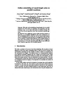
Each machine is represented by a directed tree. Every node in the tree is labelled with a window w and a length `, representing a periodic (w, `)-schedule on the machine. Each leaf might be closed or open. A closed (w, `)-leaf is associated with a (w0 , `0 )-job scheduled on this machine. In this case w ≤ w0 and ` ≥ `0 . An open (w, `)-leaf is associated with a (w, `)-periodic idle of the machine (an idle of ` slots repeated with window w). For example, the tree in Figure 1 represents a schedule of the instance I = {a = (4, 1), b = (8, 1), c = (8, 1), d = (8, 2), e = (16, 2), f = (16, 2).}.

5.3

4, 4

The implementation consists of two parts: the algorithm and the creation of an instance. 4, 3

8, 3

8, 3 8, 2

8, 1

8, 2 16, 2

16, 2

Figure 1: Tree representation of a 1-machine schedule Initially, the machine is idle. The associated tree has a single node - a (1, 1)-leaf, meaning we can schedule a job with window 1 and length 1 on this machine. An open (w, `)-leaf can be split into multiple leaves as follows: 1. Split into k open (wk, `)-leaves. For example, a (4, 2)leaf can split into three (12, 2)-leaves. 2. Split into k leaves h(w, `1 ), (w, `2 ), . . . , (w, `k )i such that Pk i=1 `i = `. For example, a (12, 8)-leaf can split into (12, 5), (12, 2) and (12, 1). Also, for any w, a (1, 1)-leaf (the root of the tree) can be replaced by a (w, w)-leaf. These rules imply a straightforward deterministic mapping of trees into a schedule. The schedule is defined recursively. The base case is the (w, w)-root representing an idle schedule of length w. A (w, `)-node that splits into k (wk, `)children represents a round-robin schedule on the children schedules, each allocated ` slots in any window of wk slots. A (w, `)-node that splits into k nodes {(w, `1 ), (w, `2 ), . . . , Pk (w, `k )} such that i=1 `i = ` represents a round-robin schedule on the children schedules, where child i is allocated `i slots in every window of w slots. The schedule represented by the tree in Figure 1 is [a, b, d, d, a, c, e, e, a, b, d, d, a, c, f, f ].

5.2

Scheduling Rule: The algorithm schedules the next (w, `)job on a leaf (v, x) that minimizes the lost bandwidth (given by 1/v − 1/w). Ties are broken in favor of leaves (v, x) with minimal x ≥ `.

1, 1

4, 1

8, 1

job to be scheduled. A (w, `)-job can be scheduled on any (w0 , x)-leaf such that w0 ≤ w and x ≥ `. Moreover, if w0 = kw00 and w00 ≤ w, a (w0 , x)-leaf can split into k (w00 , x)leaves, and one of them will be used. In both cases (split or not), if x > ` the (v, x)-leaf on which (w, `) is scheduled, splits to a closed (v, `)-leaf that is allocated to the job and to an open (v, x − `)-leaf.

The Greedy Algorithm

In the first stage of the algorithm the jobs are sorted in non-decreasing order by their window size, that is, w1 ≤ w2 ≤ . . . ≤ wn . Jobs having the same window and different lengths are sorted in non-increasing order by their lengths. That is, the w-jobs are sorted such that `1 ≥ `2 ≥ . . .. For every two jobs (w1 , `1 ) and (w2 , `2 ), the first job comes before the second one if w1 < w2 or w1 = w2 and `1 ≥ `2 . After sorting, the algorithm schedules the jobs one after the other according to the sorted order. Let (w, `) be the next

Simulation Results

Algorithm: The implementation follows directly from the algorithm specification. The implementation employs search to find the fewest trees (machines) necessary to schedule the instance. The maximum number of trees necessary is the number of jobs n in the instance while the minimum number of trees is 1. We use binary search in this range to find the fewest machines necessary. Instance Generation: In order to test the greedy algorithm, we generated random instances. Let H be the optimal number of trees for a given instance I. We generated instances with known H values to allow comparisons to the optimal. Each instance is generated from a forest of H separate (1, 1) roots, with each root generating an independent tree. Given a leaf node in a tree, the implementation randomly selects (with equal probability) to split it into k (prime number chosen randomly) children nodes, or to mark the node as frozen, prohibiting any future splits, or to split it into two children while conserving the window size in the children. The implementation uses a threshold value to terminate tree creation, and these leaves become jobs in instance I. The optimal number of trees for instance I is exactly the number of trees, H, used to create the instance. We call these non-perturbed instances since the jobs in I are exactly those generated in the tree creation process. To create instances I with less consistent window sizes, we perturb the window sizes of nodes by increasing them slightly. We denote these as perturbed instances. In order to ensure that H does not decrease, we set a limit on the differences between the original width `/w and the new width `/w0 . Specifically, the new value w0 can be between w and 1.125w (to keep modifications small) as long as P the total difference in width for all jobs remains under 1.0 ( I (`/w − `/w0 ) < 1.0). Experimental Results: We ran the greedy algorithm and the three variations on 20 non-perturbed instances and 20 perturbed instances for H between 5 and 100 (stepping by 5). The three variations sort the jobs within an instance in different ways before using the scheduling routine of the greedy algorithm. The first variation, called Demand, sorts the jobs according to their widths `/w. The Most demanding jobs (larger `/w) are scheduled first. Ties are broken in favor of small w. The second variation, called Length, sorts jobs by length, with longer jobs scheduled first, and ties are broken in favor of small w. In the final variation, Online, the jobs are shuffled randomly and scheduled in the resulting order.

Average Differences For Non−Perturbed Instances 80

Orig Demand Length Online

Average of (Num Machines − H)

70

60

50

40

30

20

10

0

0

10

20

30

40

50

60

70

80

90

100

90

100

H (Optimal) Average Differences For Perturbed Instances 180

Average of (Num Machines − H)

160

Orig Demand Length Online

140

120

100

80

60

40

20

0

0

10

20

30

40

50

60

70

80

H (Optimal)

Figure 2: For non-perturbed (top) and perturbed (bottom) instances: Shows the average difference (20 runs per H) in number of machines used and the optimal number of machines (H). The top of figure 2 shows the results for all four algorithms (Orig, Demand, Length, Online) for non-perturbed instances. The average differences between the number of machines scheduled and H are shown. In every experimental run, the original greedy algorithm used the fewest machines of all four variations and used H or H + 1 machines. The results are similar for perturbed instances as shown in Figure 2 (bottom), with the original greedy algorithm using the fewest machines. For the Demand, Length, and Online versions, the average difference for each H is roughly twice the non-perturbed results. The original algorithm used between H and H + 3 machines in every experimental run. For H greater than 30 the original greedy is usually optimal.

6.

OPEN PROBLEMS

Can the approximation factor 8 be improved? Alternatively, is there a C > 1 for which a C-approximation is NP-hard? These questions also apply to the special cases of thrift schedules and windows scheduling of power-2 instances. The optimal algorithm presented in this paper for power-2 instances is for thrift schedules. Is it NP-hard to find a non-thrift optimal schedule for these instances? As shown in the thriftiness paradox, the optimal schedule is not necessarily thrift. The greedy algorithm performs very well in practice. Is there any theoretical bound on its performance? Are there better natural algorithms for practical instances?

All of our solutions and previous solutions to the original windows scheduling do not use migrations. That is, a particular job is scheduled only on one machine. It is open to see if solutions with migrations perform better. Thrift schedules and the generalized windows scheduling are special cases of a general problem in which jobs may be scheduled with some jitter. That is, job i is associated with jitter parameters jiub and jilb and the window between any two consecutive executions of job i must be no smaller than wi − jilb and no larger than wi + jiub . In a thrift schedule both jitter parameters equal 0 and in the generalized windows scheduling problem jiub = 0 and jilb = wi −1. This generalization is motivated by maintenance problems in which jobs cannot get the service too often.

7.

REFERENCES

[1] S. Acharya, M. J. Franklin, and S. Zdonik. Dissemination-based data delivery using broadcast disks. IEEE Personal Comm., 2(6):50–60, 1995. [2] H. Ammar and J. W. Wong. The design of teletext broadcast cycles. Performance Evaluation, 5(4):235–242, 1985. [3] A. Bar-Noy, R. Bhatia, J. Naor, and B. Schieber. Minimizing service and operation costs of periodic scheduling. Mathematics of Operations Research (MOR), 27(3):518–544, 2002. [4] A. Bar-Noy and R. E. Ladner. Windows scheduling problems for broadcast systems. SIAM Journal on Computing, 32(4): 1091-1113, 2003. [5] A. Bar-Noy, R. E. Ladner, and T. Tamir. Scheduling techniques for media-on-demand. In Proceedings of the 14-th ACM-SIAM Symp. on Discrete Algorithms (SODA), 791–800, 2003. [6] A. Bar-Noy, R. E. Ladner, and T. Tamir. Windows scheduling as a restricted version of bin packing. In Proceedings of the 15-th ACM-SIAM Symp. on Discrete Algorithms (SODA), 217–226, 2004. [7] A. Bar-Noy, J. Naor, and B. Schieber. Pushing dependent data in clients-providers-servers systems. Wireless Networks journal, 9(5):175–186, 2003. [8] A. Bar-Noy, A. Nisgav, and B. Patt-Shamir. Nearly optimal perfectly-periodic schedules. Distributed Computing, 15(4):207–220, 2002. [9] S. K. Baruah, N. K. Cohen, C. G. Plaxton, and D. A. Varvel. Proportionate progress: a notion of fairness in resource allocation. Algorithmica, 15:600–625, 1996. [10] S. K. Baruah S-S. Lin. Pfair Scheduling of Generalized Pinwheel Task Systems IEEE Transactions on Computers, 47(7):812–816, 1998. [11] Z. Brakerski, A. Nisgav, and B. Patt-Shamir. General perfectly periodic scheduling. In Proceedings of the 21-st ACM Symposium on Principles of Distributed Computing (PODC), 163–172, 2002. [12] Y. Chan and F. Chin. Schedulers for larger classes of pinwheel instances. Algorithmica, 9:425–462, 1993. [13] E. G. Coffman, M. R. Garey, and D. S. Johnson. Approximation algorithms for bin packing: a survey. Approximation Algorithms for NP-Hard Problems, D. Hochbaum (editor), PWS Publishing, Boston (1996), 46–93.

[14] L. Engebretsen and M. Sudan. Harmonic broadcasting is optimal. In Proc. of the 13-th ACM-SIAM Symposium on Discrete Algorithms, 431–432, 2002. [15] W. S Evans, D. G. Kirkpatrick. Optimally scheduling video-on-demand to minimize delay when server and receiver bandwidth may differ. In Proc. of the 15-th ACM-SIAM Symposium on Discrete Algorithms (SODA), 1041–1049, 2004. [16] E. A. Feinberg, M. Bender, M. Curry, D. Huang, T. Koutsoudis, and J. Bernstein. Sensor resource management for an airborne early warning radar. In Proceedings of SPIE The International Society of Optical Engineering, 145–156, 2002. [17] E. A. Feinberg and M. Curry. Online scheduling: generalized pinwheel problem. In Proceedings of the 42-nd IEEE Conference on Decision and Control (CDC), 4333–4338, 2003. [18] M.R. Garey and D.S. Johnson, Computers and Intractability: A guide to the theory of NP-completeness, W. H. Freeman and Company, San Francisco, 1979. [19] V. Gondhalekar, R. Jain, and J. Werth. Scheduling on airdisks: efficient access to personalized information services via periodic wireless data broadcast. IEEE International Conference on Communications (ICC), 3:1276–1280, 1997. [20] L. Gao, J. Kurose, and D. Towsley. Efficient schemes for broadcasting popular videos. Multimedia Systems, 8(4): 284–294, 2002. [21] R. Holte, A. Mok, L. Rosier, I. Tulchinsky, and D. Varvel. The pinwheel: A real-time scheduling problem. In Proc. of the 22-nd Hawaii International Conference on System Sciences, 693–702, 1989. [22] R. Holte, L. Rosier, I. Tulchinsky, and D. Varvel. Pinwheel scheduling with two distinct numbers. Theoretical Computer Science, 100:105–135, 1992. [23] K. A. Hua and S. Sheu. An efficient periodic broadcast technique for digital video libraries. Multimedia Tools and Applications, 10(2/3):157–177, 2000. [24] L. Juhn and L. Tseng. Harmonic broadcasting for video-on-demand service. IEEE Transactions on Broadcasting, 43(3):268–271, 1997. [25] C. Kenyon and N. Schabanel. The data broadcast problem with non-uniform transmission times. Algorithmica, 35(2):146–175, 2003. [26] C. Kenyon, N. Schabanel, and N. E. Young. Polynomial-time approximation scheme for data broadcast. In Proc. of the 32-nd ACM Symposium on Theory of Computing (STOC), 659–666, 2000. [27] C. L. Liu and W. Laylend. Scheduling algorithms for multiprogramming in a hard real-time environment. Journal of the ACM, 20(1):46–61, 1973. [28] R. Tijdeman. The chairman assignment problem. Discrete Mathematics, 32:323–330, 1980. [29] W. F. Vega and G .S. Leuker. Bin packing can be solved within 1 + ε in linear time. Combinatorica, 1:349–355, 1981. [30] S. Viswanathan and T. Imielinski. Metropolitan area video-on-demand service using pyramid broadcasting. ACM Multimedia Systems Journal, 4(3):197–208, 1996.