Wireless Localization Using Self-Organizing Maps Gianni Giorgetti
∗
Dip. Elettronica e Telecom. Università degli Studi di Firenze, ITALY
[email protected]
Sandeep K. S. Gupta IMPACT LAB School Comput. & Info. Arizona State University
[email protected] [email protected]
ABSTRACT Localization is an essential service for many wireless sensor network applications. While several localization schemes rely on anchor nodes and range measurements to achieve fine-grained positioning, we propose a range-free, anchorfree solution that works using connectivity information only. The approach, suitable for deployments with strict cost constraints, is based on the neural network paradigm of SelfOrganizing Maps (SOM). We present a lightweight SOMbased algorithm to compute virtual coordinates that are effective for location-aided routing. This algorithm can also exploit the location information, if available, of few anchor nodes to compute absolute positions. Results of extensive simulations show improvements over the popular MultiDimensional Scaling (MDS) scheme, especially for networks with low connectivity, which are intrinsically harder to localize, and in presence of irregular radio pattern or anisotropic deployment. We analytically demonstrate that the proposed scheme has low computation and communication overheads; hence, making it suitable for resource-constrained networks.
Categories and Subject Descriptors C.2 [Computer Communication Networks]: Network Protocols
General Terms Algorithms, Performance, Design.
Keywords Self-Organizing Maps, Localization, Wireless Sensor Networks.
1.
Gianfranco Manes
Dip. Elettronica e Telecom. Università degli Studi di Firenze, ITALY
INTRODUCTION
In the era of pervasive computing, position-awareness is rapidly becoming a key feature in many applications [1]. ∗The author is also affiliated with the Electrical Engineering Department at Arizona State University.
Permission to make digital or hard copies of all or part of this work for personal or classroom use is granted without fee provided that copies are not made or distributed for profit or commercial advantage and that copies bear this notice and the full citation on the first page. To copy otherwise, to republish, to post on servers or to redistribute to lists, requires prior specific permission and/or a fee. IPSN’07, April 25-27, 2007, Cambridge, Massachusetts, USA. Copyright 2007 ACM 978-1-59593-638-7/07/0004 ...$5.00.
This trend is confirmed by the fast growth of the Global Positioning System (GPS) that has recently invaded the consumer market. Once restricted to military applications, GPS receivers are now common on cars, trucks, PDAs and cell phones. With an estimated 14 million units sold in 2006 [5], the success of this technology underlines the importance of locating people and things in a world where computation and communication are becoming ubiquitous. Position-awareness is also of primary importance in Wireless Sensor Networks (WSN) [10], which is an enabling technology for pervasive computing. Consisting of small sensors with wireless capabilities, these networks are easy to deploy and represent a cost effective alternative to traditional wired systems. Typical applications include environmental monitoring, asset tracking, surveillance and disaster relief [2]. In each case, the data gathered by the sensors are of scarce utility unless stamped with the location of the node that collected it. For example, in precision agriculture, temperature and moisture values are correlated with position to identify micro-climate zones [40]. Knowing the sensors’ position is also critical for locating an intruder vehicle in a military application as well as to guide a team of firefighters to the location of an emergency. Finally, locations are used to support network services like geographical routing [19], location-based queries [16] and resource directories [28]. Given the importance of this information, several recent research efforts have focused on incorporating location awareness in those applications where the use of GPS is not a viable solution [15, 26]. Many of the proposed schemes assume the presence of a large number of anchor nodes or the availability of hardware for range and angle measurements. Although these configurations are simple to simulate, they are not practical to implement in applications that call for true ad hoc deployment or where cost is a major issue. We also note that many localization schemes target unrealistically large WSNs with high connectivity. While a few examples of such large, dense deployments are being experimentally evaluated within the research community [3], a recent survey [4] reveals that most of the future WSN applications will exploit small to medium networks with less than 100 nodes. Contrary to other network services, a small number of nodes and low connectivity are problematic for the existing localization schemes since determining the sensor positions becomes intrinsically harder as the number of constraints (e.g. range measurements or radio links) diminishes [13]. Motivated by these considerations, we propose a lightweight localization scheme that works without anchor nodes and does not rely on range measurements. The method,
which is based on a neural network formalism known as Self-Organizing Map (see Section 3), generates virtual coordinates that describe the relative positions of nodes. In Section 5 we demonstrate through extensive simulations that these virtual maps can be used for efficient geographic routing, with results that are very close to the case where the real coordinates are available. We also evaluate the localization error when absolute positioning is required: using only three or four anchor nodes, the virtual coordinates can be converted into absolute positions by means of a linear transformation. Although in this case we use the transformation after computing the virtual coordinates, in Section 5.5 we show an extension to the algorithm where anchor positions are actively used during the localization process, allowing for further accuracy improvements. Using this extension, the localization error drops below 0.3R (i.e. 30% of the radio range) for networks with average connectivity of only four nodes. We also evaluate the performance of the scheme when irregular radio patterns affects the connectivity among nodes or when the network has an anisotropic layout due to the presence of buildings or natural obstructions in the deployment area. Surprisingly, the scheme proves to be extremely robust and none of these factors significantly degrade the localization accuracy. The results are compared to those of the popular Multi-Dimensional Scaling (MDS) technique [39], showing substantial improvement especially for networks with low connectivity or anisotropic layout. Finally, in Section 7 we evaluate the computational and communication complexity of the solution. This analysis, in addition to benchmark tests on real hardware, shows that our lightweight implementation is suitable to solve the localization problem in resource-constrained networks.
2.
THE PROBLEM
A localization service must be able to compute the coordinates of a set of randomly deployed nodes. We restrict our attention to anchor-free and range-free schemes, meaning that none of the nodes are placed at known positions and no attempt is made to estimate the inter-node distances. Such algorithms attempt to compute a network map using only connectivity information that describes which nodes are in radio range. Interest in such approaches is due to the fact that each node can determine the set of its radio neighbors with minimal communication overhead and without needing any additional hardware (e.g. ultrasound transceiver for range measurements or GPS); thus, enabling localization in deployments where cost is of primary importance. Before analyzing the complexity of the problem, it is useful to remember that the coordinate assignment produced by an anchor-free scheme is intrinsically ambiguous - since no reference points are used, the maps produced are correct up to global translations, rotations or flipping. In addition, the result is arbitrarily scaled unless knowledge about the average communication radius is used to properly scale the map. As consequence of these ambiguities, the localization scheme will generate virtual coordinates [31] that only describe the relative locations of nodes (nodes with similar coordinates are physically close). Virtual coordinates, which can facilitate network tasks as location-based queries and proximity-based service discovery, have found prominent application in the area of geographic routing [19, 25, 37]. By knowing the relative position of nodes, geo-routing schemes
achieve efficient packet delivery without the memory overhead of table-driven protocols or the latencies of on-demand approaches. Intuitively, a localization scheme produces a coordinate assignment where neighboring nodes are within the maximum radio range and non-neighbors are further apart. Although the problem can be stated in simple terms, the solution in the general case is complex. A network with connectivity constraints can be modeled as a Unit Disk Graph (UDG) 1 and the localization problem can be posed as one of embedding an UDG in an Euclidean space. This problem is NP-Complete in one dimension and NP-hard in two dimensions [7]. Recently, the problem has been proved to be APX-hard [29], meaning that the solution cannot even be efficiently approximated. In fact, there exists node configurations for which even an optimal algorithm p cannot produce an embedding with quality better than 3/2 [24]. While this value limits the worst-case error for an optimal algorithm, localization schemes with bounded errors are very few. A recent work [31] proposes a scheme based on spreading constants √ and random projection with a bound error of O(log2.5 n log log n), where n is the number of nodes. Although this work has an appreciable theoretical value, from a practical point of viewp we are still far from approaching the theoretical bound of 3/2 [34]. Having outlined the characteristics of the problem, we propose a solution inspired by a neural network paradigm known as Self-Organizing Maps (SOMs) [21, 22]. Introduced in the early 80’s, these maps have found numerous applications in many areas such as speech recognition, data mining and bioinformatics ([20, 35] contain an extensive bibliography of SOM papers). In the next sections, after introducing the map structure and the learning algorithm, we show how the SOM formalism leads to an intuitive solution of the localization problem. Unfortunately, despite the attention received, SOMs have proved to be surprisingly resistant to mathematical characterization and convergence results are only available for the case of one-dimensional configuration of neurons [9], therefore we use extensive simulations to characterize the localization results and to compare our solution to the MDS technique.
3.
SELF-ORGANIZING MAPS
A SOM [21] is a neural network that learn application information as a set of weights associated with the neurons (nodes). In comparison with other techniques (e.g. MultiLayer Perceptron), SOMs are unique because the neurons are arranged in regular geometric structures, typically twodimensional lattices with rectangular or hexagonal patterns like the one in Figure 1a. As we will soon see, this spatial arrangement plays a central role in the training process of the maps and results in a topological organization of the information learned2 . The training of a SOM is performed in an unsupervised fashion: the map is able to learn the underlying properties of the training set without the aid of labeled samples or reward functions (hence, they are characterized as “self-organizing”). 1 A Unit Disk Graph is a graph where two node are connected iff their distance is less than 1. 2 This model vaguely resembles the structure of the cerebral cortex, where neurons are placed on a 2D surface and interact preferentially over lateral synaptic connections.
w
Neighborhood Function h( )
w jd
Weights changes
Neighboring Neurons
(a) SOM
(b) Adaptation
Figure 1: A two-dimensional map with the unit forming an hexagonal pattern. Assuming that the input samples and the map weights wj ’s are d-dimensional real valued vectors, the three phases of the training algorithm are as follows: 1. Sampling: A sample is extracted from the training set and presented to the network. We use the notation x(n) to denote the sample at current iteration. 2. Competition: The sample x(n) is compared with the map weights (there is one weight per neuron) through the use of a discriminating function f = f (x, w). The neuron that scores the maximum value wins the competition and become the Best Matching Unit (BMU). If the discriminating function is implemented using the Euclidean distance, the election rule is given by: BM U (n) = arg min kx(n) − wj (n)k . j
value of r(n) decreases with the number of iteration: a relatively large radius during the initial iterations allows the map to quickly organize the neurons, while a smaller value toward the end determines localized changes, such that different parts of the map become sensitive to different input features. The SOM technique is simple yet effective in capturing the properties of the input space and organizing them in an ordered fashion. An example of the SOM method in action is reported in Figure 2, where a 10 × 10 rectangular map is trained with random samples x(n) = [rn , gn , bn ] from the RGB color space (Figure 2a). In this case, the weight vectors have the form wj = [rj , gj , bj ] and can be displayed using the corresponding color. Figure 2b shows the initial configuration of randomly assigned weights. After training the map with a few thousand random samples, the SOM assumes the configuration shown in Figure 2c. The result shows that among the 224 colors of the input space, not only the map was able to select 100 representative samples (SOMs are vector coding techniques), but it also generated a topologically ordered representation of the color space, in the sense that similar colors were mapped to nearby locations. This property emerges as a consequence of the update rule: since adjacent neurons are subjected to similar weight changes, they eventually converge to similar values.
1 BLUE
j1 Neuron j w j2 Weight vector w j = ...
0.5
(1)
0 1
1
GREEN
3. Adaptation: Finally, the weight vectors of the BMU and its neighbors are adapted according to the following rule: wj (n + 1) = wj (n) + η(n) h(j, BM U (n))[x(n) − wj (n)]. (2) The update formula in (2) is controlled by the global learning rate parameter η and by a neighborhood function h = h(i, j) (see Figure 1b). For ensuring convergence, the learning rate η must decrease monotonically with the number of iterations. A common choice is to implement the learning rate as an exponential function that decays from ηmax to ηmin over a given number of iterations. Typically, η decreases within the range [ηmax , ηmin ] = [0.1, 0.01], while the number of iterations goes from few hundreds to several thousands depending on the size of the training set. The update rule is also controlled by the neighborhood function h = h(·, ·). This function regulates the weight changes on the basis of the map distance between BMU and the neuron being adapted. In the case of a Gaussian shaped neighborhood function, the expression of h is given by: µ ¶ distmap (i, j)2 h(i, j) = exp − , (3) 2r(n) where distmap (i, j) measures the distance on the map between two neurons. According to this expression, the magnitude of the changes is maximum for the BMU and decreases for units that are far from it. The extent of the area affected by the changes depends on the radius r(n), a global parameter that controls the “width” of the neighborhood function. As in the case of the learning rate, the
0.5
0.5 0 0
(a)
RED
(b)
(c)
Figure 2: 10×10 SOM trained with samples from the RGB color space: a) input space, b) initial weights, c) final weights.
4.
LOCALIZATION USING SOMS
At the end of the training phase, the neurons contain model vectors that are representative of the input space, therefore the map can be used as a codebook for arbitrary samples. The code is given by the weight vector that best matches (BMU) the given sample. In addition, since each BMU defines a position on the two-dimensional grid, SOM implements a projection technique3 from the input space to the plane defined by the lattice of neurons (see Figures 2a and 2c). This property has been widely exploited in many applications for data analysis and visualization of large data sets [20, 35]. More recently, SOMs have been used to implement localization schemes for mobile robots in unknown environments [17, 12]. The SOM, initially trained with information collected by on-board sensors during the exploration phase, is then used as a virtual map to translate new sensor readings into grid positions or to recognize different environments (e.g. different rooms). Ertin and Priddy [11] have used a similar approach to solve the localization problem in WSNs. In their work, synchronous readings collected by all the sensor nodes are used 3 In this sense SOM can be seen as non-linear version of the Principal Component Analysis (PCA) technique.
to build the training set for the SOM. After training the model, the localization task is performed using new sensor readings to sort nodes on the basis of their proximity to a virtual grid of nodes. Although no attempt is made to compute individual node positions, the authors suggest possible applications to the target tracking problem. Our solution is similar to [11] in the sense that it is also based on the SOM formalism, but the approach taken is rather different since it does not rely on sensor readings or time synchronization services. In addition, our scheme explicitly computes individual node positions as a result of the training phase of the map. More details on the approach used in [11] are given in Section 8. The intuition behind the proposed solution is that, with no prior information on sensor locations, the best assumptions we can make are: i) sensor nodes provide an (approximately) uniform coverage of the deployment area and ii) nodes that are within their radio range are relatively close to each other. In Section 6, we consider non-uniform deployments and the effect of irregular radio patterns, nevertheless the two assumptions (uniform coverage, radio neighbors close to each other) are realistic for many WSNs and are useful to give an intuitive illustration of our approach. To solve the problem we must therefore generate a location assignment that is approximately uniform, taking care of placing neighbor nodes close to each other. This is accomplished by associating the unknown node positions (xi , yi ) to the weights of a SOM and then training the model with random samples from an uniform distribution. As a result of the training phase, the weights (i.e. nodes position) will eventually spread to cover the sampling area and, if associated to adjacent neurons on the map, neighboring nodes will be kept close to each other. Using an approach substantially analogous to the one exposed here, SOMs has been previously applied to graph drawing [30, 6], a branch of graph theory that deals with the visualization of complex graphs. The graph layout problem is similar to the localization problem in the sense that it also seeks to find a coordinate assignment such that vertices connected by edges are positioned close to each other. However, while the evaluation of a graph layout is mostly based on aesthetic factors (e.g. uniform distribution of nodes and edge lengths, separation between graph elements, number of edge crossing, etc.), the results of the localization assignment are directly comparable with the true sensor locations. In this work we explicitly evaluate the effectiveness of SOM in producing maps similar to the ground truth and we focus on reducing the localization error.
4.1
System Model
We consider a connected network with N nodes placed at unknown locations (xi , yi )i=1,...,N . None of the nodes is equipped with hardware for position, range or angle estimation (e.g. GPS, ultrasound receivers or smart antennas) and no assumption is made regarding availability of sensors at each location. We only assume that every node can determine the set of its radio neighbors4 and can transmit this information to a central point of computation. Also, during the neighbor discovery phase, nodes use the same transmission power in the effort to ensure an approximately uniform communication range. Once the connectivity information 4 By neighbors, we mean symmetrical radio neighbors: messages from node j are received by i and vice versa.
is known, the network can be represented as an undirected graph Gnet = (V, E), where two vertices are connected if the corresponding nodes are radio neighbors. The graph also serves to introduce the hop distance metric d = disthop (·, ·) defined as the length of the shortest path connecting two nodes.
4.2
Modified SOM Model
The core of the SOM technique is the update rule defined in (2). In that expression, the neighborhood function h(·, ·) takes into account the spatial arrangement of the neurons through the map distance distmap (·, ·). Now we note that, as long as a distance function between two elements on the map is provided, the regular lattice can be replaced by an arbitrary structure of interconnected neurons. Consequently, we modify the original SOM architecture by using the network graph in place of the lattice of neurons and exchanging the map distance with the hop distance disthop (·, ·). The new neighborhood function is given by: µ ¶ disthop (i, j)2 h(i, j) = exp − . (4) 2r(n) Having defined the new neighborhood function, the training algorithm illustrated in Section 3 can be applied to the localization problem. In this modified SOM model, neurons are located on the vertices of Gnet , hence we have a direct correspondence between the neurons and the network nodes. The weight vector associated with each neuron/node j has the form wj = (xj , yj ). This vector, initially picked at random, will eventually contain the estimated location for the corresponding node.
4.3
Localization Algorithm
Since the proposed algorithm is centralized, each node needs to communicate the list of its radio neighbors to the unit in charge of the computation. This information is necessary first to build the adjacency matrix of Gnet , and then to compute the hop-count distances between each pair of network nodes, which are stored in a matrix HC with elements given by {hc}i,j = distmap (i, j). The matrix HC is the only input parameter required by the localization algorithm. According to the scheme of Section 3, the weight vectors (xj , yj ) are initialized with random numbers and then trained with a set of input samples. Since we are using only connectivity information, we are free to work in a relative reference system where absolute coordinates are not important. In light of this model, we can easily generate the training set by sampling random points from an arbitrary uniform distribution (e.g. 0 ≤ x, y ≤ 1). This fact greatly simplifies the implementation of the algorithm since the localization task can be performed without having to rely on any other external information (e.g. network’s physical dimensions or sensor readings like in [11]). Algorithm 1 contains the pseudo-code of the localization scheme. In the proposed scheme, the learning parameter η(n) and the radius r(n) are decreased linearly with the number of iterations (see lines 7 and 8). As a side note, we mention that, as the radius r(n) shrinks, the level of adaptation for neurons far from the BMU becomes negligible, so the update rule (line 13) can be more efficiently restricted to neurons within a short hop distance from the BMU. In Section 5.4, after defining the simulation setup and evaluation metric for the algorithm, we provide additional
considerations on the weight initialization and the number of iterations required by the algorithm. Algorithm 1: SOM Based Localization Input: matrix Hc : hop count distances among nodes Output: (xj , yj )j=1,...,N : node positions % Initialization 1: [ηmax ; ηmin ] = [0.1; 0.01] 2: [rmax ; rmin ] = [(max HC (i, j))/2; 0.001] i,j
deviation σPE = {0.1, 0.2, 0.3, 0.4, 0.5} r. Figure 3 reports two topologies for different values of the placement error. Communication Radius, R: The maximum communication radius is chosen as a function of the spacing factor r: R = {1.25, 1.5, 1.75, 2.0, 2.25} r. In this first set of simulations, we consider two nodes as neighbors if their distance is less than R. We analyze the effect of irregular radio pattern in Section 6.1. 1.2 95 91
1
92
81 71
0.8
82 72
9: 10:
(x, y) = random() BM U = arg min k(x, y) − (xj , yj )k
11: 12:
for all network nodes j do ´ ³ Hc (BM U,j)2 h = exp − 2r(n)
j
13: (xj , yj ) += η(n)h[(x, y) − (xj , yj )] 14: end for 15: end for
SIMULATIONS
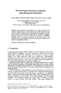
In this section, we report the results of the simulations used to validate our localization scheme. Since we are interested in evaluating our scheme’s performance in localizing small to medium size networks (10 - 100 nodes) with low connectivity, we need to impose some constraints on how the random topologies are generated. We refrain from purely random deployments (coordinates selected as i.i.d. random numbers) for two reasons: i) it is unrealistic to assume that nodes will be positioned independently from each other and ii) in purely random deployments, the probability to obtain connected networks rapidly decreases to zero as we reduce the communication range [23]. Since it is difficult to generate meaningful low-connectivity topologies, we consider a model in which the node density is kept roughly uniform by having the nodes positioned on the intersection points of a grid with rows and columns spaced by a factor r. We capture the nature of an ad hoc deployment by perturbing the positions with random noise and allowing for large placement errors.
5.1
Simulation Parameters
The parameters used to generate our simulation are the following: Number of nodes, N: We simulated networks with 16, 25, 36, 64, 81 and 100 nodes. Placement Error, : The initial positions are given √ σPE√ by a regular grid of N × N elements spaced by a factor r. Node positions are obtained by perturbing the grid positions with Gaussian noise having zero mean and standard
12
11
33
56 55 45
24
3
36
58
47
48
15 5
4
75 65
62 5253
51 0.4
40
63 43
64 55
29
0.2
19 20
18
0
0.2
0.4
0.6
60 59
48
37
38
49 39
50 40
27 15
13
11
80
70
69
35 25
12
26 16
18
17
30 28 29
20
14
9 10
8
0.8
68 78
47
36
2
0
5
−0.2 −0.2
56 46
45
2324 22
1
58 66 67 57
34 21
30
100 90 89 79
32 33
41
28
54 44
42 31
99
88 87 77 76
0.6
50
39
17
6 7
61
98 97
86 85
84
73
59
37 27
16
70
49
26
25 14
13
2
57
38 35
34 23
46
69
94 93 74
71 72
0.8
60
44
83 92
90 79 80
67 68
82 91
89 78
77
66
1
100
96
81
4 3 1
1.2
−0.2 −0.2
(a) σP E = 0.2r
0
0.2
0.4
6
0.6
7
8
9
19 10
0.8
1
1.2
(b) σP E = 0.5r
Figure 3: Two 100-node networks with different placement errors. The algorithm was evaluated by generating 50 networks for each combination of the above parameters. After discarding disconnected networks, the number of simulated topologies is 9630, with an average connectivity of 6.98. The results presented in the following sections were obtained by executing 2000 iterations of the algorithm presented in Section 4.3.
5.2 5.
21 22
1
65
76
54
32
98 99 88
87
75
64
53 43
42
31
0.2
84
63
52 51 41
96 86
74 62
0.4
95
97
85
73
0.6
0
% Main Loop 6: for n = 1 : to n_iter-1 do 7: η(n) = ηmax − n(ηmax − ηmin )/(n_iter − 1) 8: r(n) = rmax − n(rmax − rmin )/(n_iter − 1)
9394 83
61
3: for all nodes n do 4: (xn , yn ) = random() 5: end for
100 Nodes; Radius = 0.194444; Avg Connectivity = 6.76
100 Nodes; Radius = 0.194444; Avg Connectivity = 7.06 1.2
Virtual Coordinates
The SOM based scheme is truly an anchor-free, range-free algorithm in the sense that it can generate virtual coordinates without relying on anchor nodes or distance measurements. Since the virtual coordinates cannot be compared to the true network coordinates, we use the delivery ratio of a greedy routing algorithm as evaluation metric. At each hop, the routing scheme forwards the packet to the neighbor node that is closer to the recipient of the message, according to the rule: next_hop = arg min k(xn , yn ) − (xdest , ydest )k , n
where (xn , yn ) are the virtual coordinates of the neighboring nodes and (xdest , ydest ) are those of the destination. Although the scheme is extremely unrefined (it simply gives up if it is unable to get closer to the destination), it is still useful to define a baseline for the performance achievable using more advanced schemes (e.g. GPRS [19]). Using the simulation setup previously introduced, we have compared the performance of our approach with the results of MDS, a popular projection technique that has been successfully applied to the localization problem in WSNs [39, 38, 18]. Figure 4a reports the percentage of packets successfully delivered using the greedy algorithm that operates on the basis of the relative maps generated by SOM and MDS. The results show that the virtual coordinates produced by both methods are effective when used for geographical routing, with a delivery ratio that is very close to that obtained using the true network coordinates. Similarly, the length of the routing path does not differ substantially from the case where the true node positions are known to the routing scheme (graph is not shown).
Greedy GeoRouting Delivery Ratio
1
80
0.6
MDS − Absolute Avg. Err (R)
1
σ = 10% r PE σPE = 20% r σPE = 30% r σ = 40% r PE σ = 50% r
0.8
90
Avg Err(R)
Delivery Ratio (%)
100
SOM − Absolute Avg. Err (R)
σ = 10% r PE σ = 20% r PE σ = 30% r PE σ = 40% r PE σ = 50% r PE
0.8 Avg Err(R)
110
PE
0.4
0.6 0.4
70 True Coord SOM MDS
60 50 2
4
6 8 10 Network Connectivity
12
0.2
0.2
14
0 0
20
(a) Delivery Ratio
40 60 Network Size
80
0 0
100
20
40 60 Network Size
(b) SOM
80
100
(c) MDS
Figure 4: a) Delivery ratio using virtual coordinates and b,c) Average Error (R) as function of network size for SOM and MDS.
5.3
Absolute Coordinates
Virtual coordinates can be computed solely on the basis of connectivity information and are useful for important network tasks such as packet routing. Nevertheless, there are applications where absolute positions are required (e.g. a WSN to support a first responder team that needs to quickly locate the emergency scene). In order to convert relative node positions into absolute coordinates, at least three anchor points are needed for the bidimensional case. In this section, we have used four anchor nodes on the perimeter of the map to resolve rotational, translational and flipping ambiguities and align the map to an absolute coordinate system. As a result of this transformation, the computed positions can be compared with the true positions and the localization error can be expressed quantitatively. Figures 4b and 4c show the error of SOM and MDS for different network sizes and placement errors. The error is expressed as a value relative to the communication range R. As expected, the accuracy of the localization schemes decreases as the placement error on the map increases. We note that while MDS works by actively using the hop-count distances between each pair of nodes, and thus it works better for larger and denser networks (where the number of constraints is higher), SOM is based on localized constrains and works better for smaller networks.
5.4
Weight Initialization and Convergence
Having defined the simulation parameters and the localization error, we analyze the effect of weights initialization and number of iterations on the algorithm’s performance. Weight initialization influences both the convergence speed and the localization accuracy. In Sections 3 and 4 we stated that weights are initialized at random (usually with samples from the input set or other small values). In our simulations we have verified that this approach works well on average, but there are few occurrences where the final error is large (> 1.0R). Figure 6 shows: a) a random topology b) the initial weight configuration and c) a case where the localization algorithm produced a substantially acceptable result. On the other hand, Figure 6d shows an occurrence where the algorithm failed to converge to an acceptable solution for the same network topology. Although the relative positions of the majority of nodes are correct with respect to each other, the network is “twisted”, with the nodes of the upper
25 Nodes; Radius = 0.412500; Avg Connectivity = 5.36
25 Nodes; Radius = 0.412500; Avg Connectivity = 5.36 1.2
22
23
1
25
24
21
1 5 12
4
6 24
0.8
16
0.8
20
17
10
1
19
18
18
16
23 9 19
0.6
0.6
7
21
8
14 11 12
20
15
13
3
13
2 0.4
0.4
11 14
8
7
6
10
15 0.2
9
0.2
22 25
4 0
3
2
1
−0.2 −0.2
0
0.2
0.6
0.8
17
0
5
0.4
1
1.2
−0.2 −0.2
0
(a) Ground Truth
0.2
1
0.6
0.8
1
1.2
25 Nodes; Radius = 0.412500; Avg Connectivity = 5.36
25 Nodes; Radius = 0.412500; Avg Connectivity = 5.36
1.4
1.4
1.2
0.4
(b) Random Init.
22
21
25 23 24
23
21
25 24
19
17
16
22
1.2
20
18
19
17
16
1
20
18
0.8
0.8 11
0.6
13
12
14
15
13 0.6
14 15 12 11
0.4 7
6
8
0.4 9
0.2
10
3 0
2
1
4
0
0.2
0.4
0.6
0.8
1
1.2
0 −1.4
6
10 3
5 −0.2 −0.2
7
8
9
0.2
5
4 −1.2
−1
−0.8
−0.6
−0.4
2
1 −0.2
0
(d) Conv. ERR
(c) Conv. OK
Figure 6: Localization convergence. half in inverse order respect to the lower half. Such problem is caused by unfortunate initial weight configurations that determine a topological flipping of large blocks of nodes. In our experiments we found that the occurrence of such cases can be greatly reduced by initializing the weights with values lying on a straight line. The initialization rule is given by: (xi , yi ) =
Hc (o, i) , max Hc (o, j)
(5)
j
where o identifies a node placed on the perimeter of the map. According to the equation, weights are initially aligned along a line starting from (0, 0), the position of node o, and ending at (1, 1), the position of the node with maximum hop count distance from o. This scheme, which partially sorts the initial node positions, helps in reducing the final localization error as well as the occurrence of “twisted” networks. In our simulations we found that the proposed solution reduces the average localization error by about 43% with respect to random initializations, while the pergentage of networks with final error > 0.5R is only 10.6%, against 31.5% for random initialization and 20.12% for MDS.
1
1 MDS SOM SOM A 3 SOM4A
0.4
0.6 0.4
0 2
4
6 8 10 Network Connectivity
12
0 2
(a) DOI = 0.0
4
0.6 0.4 0.2
0.2
0.2
MDS SOM SOM3A SOM A
0.8 Avg Err (R)
0.6
MDS SOM SOM A 3 SOM4A
0.8 Avg Err (R)
0.8 Avg Err (R)
Avg. Err (R)
Avg. Err (R)
Avg. Err (R) 1
4
6 8 10 Network Connectivity
(b) DOI = 0.2
12
0 2
4
6 8 10 Network Connectivity
12
(c) DOI = 0.4
Figure 5: Average Error (R) as function of network connectivity for different values of radio pattern DOI. The localization accuracy also depends on the number of iterations used in the algorithm. Figure 7 reports the average localization error for a test set containing 100 topologies generated using the simulation parameters defined in Section 5.1. We note that error rapidly decreases during the first 500 to 1000 iterations and then only reduces marginally. Avg. Err(R) vs. N. of Iterations 1 Random Weights Straight Line
Avg. Err (R)
0.8 0.6 0.4 0.2 0 0
1000
2000 Iterations
3000
4000
Figure 7: Average Error (R) as function of the number of iterations (results averaged over 100 random topologies).
5.5
show a substantial improvement in the localization accuracy: using four anchor nodes during the computation (SOM_4A) reduces the average localization error by about 30% with respect to the basic SOM algorithm, while the percentage of networks with localization error >0.5% drops to only 3.15% of the total cases. Figure 5a reports the results for various values of network connectivity. The plot shows that the SOM algorithm significantly outperforms MDS when the network connectivity is low, with an average error reduction of 43% for networks with connectivity between 3 and 10 (using SOM_4A). The explanation is that SOM is “less aggressive” in the use of node distances. The effect of the neighborhood function h(·, ·) is such that the distance constraints among nearby sensors are weighted more than those of nodes several hops away. Consequently, the SOM scheme is less sensitive to condition of low connectivity, where high values of the hop count distance between two nodes do not necessarily imply that nodes are far from each other.
Exploiting Anchor Information
In previous sections, the maps generated by SOM and MDS have been scaled and oriented by using the position of four anchor nodes. However, the structure of our approach is such that anchors’ information (if available) can be exploited during the training phase of the map, with valuable effects on the final results. The modification to the algorithm involve two points: i) coordinates of anchor nodes are never updated (since they are already correct) and ii) whenever an anchor node is elected as BMU, the sample at current iteration is replaced with the anchor’s position. The two modifications have the effect that anchor nodes not only remain in their position, but they also facilitate the map organization during the initial iterations. In addition, if the number of anchors is equal or greater than three, the method generates absolute coordinates without needing any further transformations. We have evaluated the performance of the algorithm using a priori knowledge of three and four anchor nodes (SOM_3A and SOM_4A respectively). The results
6. ANISOTROPIC DEPLOYMENTS Our localization scheme has been derived under the assumptions of approximately uniform deployment and communication range. In this section we use simulations to evaluate the effect of irregular radio patterns and anisotropic deployment on the algorithm’s performance.
6.1
Irregular Radio Pattern
The results reported in the previous section were obtained assuming an idealized radio model, where two nodes are neighbors iff their distance is equal to or less than the communication range R. This assumption is very strong and does not take into account the nature of radio propagation in the space. To get an insight on the effect of multi-path, scattering and shadowing on the transmission range, we repeated experiments using a less ideal radio model. In particular we took into account the influence of an additional parameter, the Degree of Irregularity (DOI) with values 0.2 and 0.4. A DOI equal to 0.4 means that the effective transmission range for each sensor is uniformly drawn from the interval [0.6R - 1.4R], where R is the average radio range. In Figures 5b and 5c we report the experimental results for DOI = 0.2 and DOI = 0.4, showing that the localization error does not significantly increase in conditions of irregular radio pattern (especially in the SOM_4A modification).
6.2
Anisotropic Networks
In addition to considering irregular radio patterns, we have simulated networks with anisotropic layouts resulting from the presence of large obstacles (e.g. buildings) in the region of the deployment. It is known that under such scenarios MDS, similar to the case of low connectivity, does not perform well. The reason is that MDS uses the hop count as a distance measure between each pair of nodes. While this approach works well when the path connecting two nodes lies approximately on a straight line, it generates large errors in the presence of obstacles. In this case two nodes can be physically close even if their hop distance is large. The large error in the case of anisotropic networks has motivated alternative approaches where MDS is used to compute small local maps that are then stitched together into a global map [39, 18]. Although this approach can be useful to solve the problem in a distributed manner, the process of map stitching greatly increases the complexity of the solution and is susceptible to large errors when the network connectivity is low. It would be useful to have a scheme capable of localizing irregular networks without having to partition the map and encumber the complexity of map stitching. To validate the performance of the SOM algorithm we have evaluated anisotropic deployments obtained by randomly placing the nodes around few obstacles. Two sample topologies are represented in Figures 8a and 8b.
72 Nodes ; Ra dius = 0.225000; Avg Conne ctivity = 7.44
59 Nodes ; Ra dius = 0.225000; Avg Connec tivity = 5.73
1.2
1.2
65 1
0.8
6667 58
64 55 46
56
48 43
47 0.6
0.4
0.2
40 41 37
-0.2 -0.2
1
0
70 61 52
60
51
44
1
72
71
56
62 63 53
0.8
54 0.6
21
2223 13 14
0.2
5 3
46
40 34
4
0.4
25
15
16
36 35 26 27 18 17
35 26
8
6
0.8
0.2
0
(a) “C” deployment
8
18
1.2
-0.2 -0.2
1
0
2
0.2
10 3
29
28
48
43 3738
30 31
20 1213
19
17 9
9
1
27 16
7
0.6
25
24
55
47 42
36
33
34
54
53
41
39
0.4
32 33 24
31
12
2
52
44 45
45
30
20
58 57 51 50
49
39
11 0
59
69
42
28 38 29 19 10
68 59 50 49
57
21 22
32 23 14 15
11 4
5
6 7
0.4
0.6
0.8
1
1.2
(b) “W” deployment
Figure 8: Anisotropic networks. SOM and MDS were tested by simulating 200 random networks for both the “C” and “W” shaped maps with connectivity between 4.6 and 6.8. As in the previous simulation, we evaluated the average error after orienting the map using four anchor points on the perimeter. For the MDS localization scheme, the simulation results confirmed our expectation: the average final error was large in both cases, 1.56R for the C-shaped and 1.32R for the W-shaped network. The SOM algorithm did not suffer the same problem and produced results with the accuracy comparable to the case of uniform networks: 0.33R for the C-shaped network and 0.38R for the W-shaped one, with an average error reduction of 75% with respect to MDS. As explained previously, the better results are due to the fact that SOM mainly exploits the constraints derived by neighbors nodes that are placed few hops away from each other; consequently, it does not incur in large errors trying to relate the position of nodes that are several hops away. Figure 9 presents four sample maps generated by the MDS and SOM algorithm for the “C” and “W” topologies to give a qualitative illustration of the results.
7.
COMPUTATIONAL COMPLEXITY
Recently, several research efforts have been directed toward the study of distributed localization algorithms. This interest is motivated by the fact that centralized computation is not viable in the following circumstances: 1) the communication overhead to transfer the input data to a central unit is too high, 2) none of the devices in the system possess the computational resources to compute the whole solution, 3) the result is critical and introducing a single point of failure puts the reliability or security of the system in jeopardy. In this section we analyze the overhead of our scheme, showing that the SOM approach, although centralized, does not suffer from the above mentioned drawbacks and is suitable for highly constrained deployments. The algorithm operates on the basis of connectivity information, therefore each sensor needs to communicate the set of its radio neighbors to the unit in charge of the computation. Assuming that node IDs are coded using two bytes (up to 65536 nodes), the information can be transmitted using a fairly small size radio messages. For example, the average connectivity of the networks in our simulations was less than 7, thus, on average, only 14 bytes need to be transmitted by each node. Since the amount of data can be further reduced by means of data aggregation techniques, the overhead to transfer the initial information to the central node does not pose a problem for many cases of practical interest. Having received the neighbor sets, the data is used to generate the adjacency matrix of the network graph requiring [N (N − 1)/2]/8 bytes5 and then to compute the table Hc with the hop count distances between nodes. The solution can be obtained by repeating N executions of the popular Dijkstra’s algorithm or using the Floyd’s scheme. The complexity is O(N 3 ) in both cases, while the table needs enough storage space for N (N − 1)/2 elements. The memory requirements for this table can be reduced by taking into account the maximum hop count distance between any two nodes (i.e. the network diameter). In our simulations, the average diameter was equal to 6.19 with a maximum value of 16. Using 4 bits to code the hop-count distances6 , the size of the table is reduced to N (N − 1)/4 bytes of memory. Finally, we need to reserve the memory space to hold the coordinates of the sensor nodes (i.e. the SOM weights). Assuming, that each coordinate is represented with 2 bytes, the total occupation is 4N bytes. As for the computational complexity of our approach, the iterative solution allows a trade-off between accuracy and execution time (cf. Section 5.4). Each iteration determines the BMU (requiring N comparisons), and then applies the update rule (2) to the map weights. Considering that the radius of the neighborhood function shrinks from a value initially equal to the network radius and then goes to zero, the average number of weight updates is N/2. While the algorithm executes in a few second on a PC, we have implemented a TinyOS [27] version to test the scheme on WSN nodes. The code was executed using TelosB [36], a low cost, commercially available sensor node. The board 5 We recall that the graph is undirected, so both the adjacency matrix and the hop count table are symmetric. 6 We note that even if some hop count distance exceeds the upper limit allowed, replacing this value with the upper limit does not have a noticeable impact on the algorithm because the interactions between units far from each other are very weak.
72 Nodes; Radius = 0.225000; Avg Connectivity = 7.44
60 Nodes; Radius = 0.250000; Avg Connectivity = 6.67
1.2
72 Nodes; Radius = 0.225000; Avg Connectivity = 7.44
1.2
65 66 67 1
58
55
60
48
44
51
46
0.8
71
50
59 60
50 51
1
0.8
55 54 5352
46
65
0.8
49
48
40
0.6
40
23
0.4
29 30
2838 19
0.2
32
4
1
−0.2 −0.2
0
5
9 10 0
1
3
29
27 26
46 40
0.4
2
1314
4 5
8
12
7
46
0.6
41 42 34 35 26 25 2829 36 16
6
3
5
23
32
14
23 1322 5
7
27 19
17 11
34 25
10 9
0.2
26 35 17 18
16 8
6
18
15
0.4
2433 15
2736
9
47
0.4
0.6
0.8
1
(a) SOM: “C” net
1.2
−0.2 −0.2
0
0.2
0.4
0.6
0.8
1
(b) SOM: “W” net
1.2
−0.2 −0.2
0
0.2
0.4
0.6
0.8
1
1.2
1.4
−0.2 −1
(c) MDS: “C” net
59
43 44 38
30 13 20 22 21 31 12 7
2 8 6
7 0.2
54 49
37 14
4 1
0
60
55 48
40 39 32 33 3 24
31
12 4
0
8
51 45 50
2930 21
11
0.2
56 57
0.8
39
37 38 20
21
49
48 43
47 4142
1
22
20
28
19 10
31
28
19
11 2
30
36 35 18
17
9
16
6
3
2
0.2
18 17
15
13 12
11 0
16
27
26 35
25 34
14
34 25
15
36
33 24 23 22
21
10
57
56
38
42 41
0.4
31 20
33 24
0.6
37
39
41 42 37
1.2
6044 1
44 43
47
61 52 51
68 50 59
66 67 58 5564
32
45 6263 5471 53
69
39
0.6
58 1.4
70
1
58
45
43
47
1.6
72
57 56
72
63 52 62 53 54 45
60 Nodes; Radius = 0.250000; Avg Connectivity = 6.67
1.2
70 61
49
57
56
69
68 59
64
52 53 −0.5
0
0.5
1
1.5
(d) MDS: “W” net
Figure 9: Sample results for anisotropic layouts: in this case, the SOM algorithm reduces the average localization error of 75% with respect to MDS.
Table 1: Memory requirements and execution time of the SOM algorithm on a TelosB node. N. Nodes Memory Exec. Hc Exec. 1000 iter. 36 0.42 KB 1 sec 62 sec 64 1.48 KB 6 sec 102 sec 100 3.42 KB 22 sec 156 sec
is equipped with Texas Instrument MSP430 F1611, a low power 16-bit RISC microcontroller featuring 10KB of RAM, 48KB of code memory and an internal oscillator working at the frequency of 8MHz. The algorithm was implemented as reported in Section 4.3, with the only exception that the Gaussian neighborhood function was replaced with a triangular function, which produces similar results using much less computation. Table 1 reports the memory occupation of the data structures described above and the execution time to compute the table Hc and then to perform 1000 iterations of the localization algorithm. As can be seen from the table, the limited hardware resources of an inexpensive sensor node are sufficient to generate a solution within a limited amount of time even for networks of 100 nodes. During the computation, the radio can be turned off and the microcontroller draws only few milliamp of current, with negligible impact on the energy budget of the sensor node. Since the algorithm runs with limited overhead on the same hardware used to implement the sensing task, the system reliability can be improved by simply running the computation on a few back-up units.
8.
RELATED WORK
Several localization techniques have been proposed in the past years. Although many schemes use TDOA (Time Difference of Arrival), Angle of Arrival (AoA) or analysis of the RSSI signal to obtain constraints on the position of neighboring nodes, some schemes are range-free and use connectivity information only. One of the first examples of such a technique is the “GPS-Less” [8] positioning system, where nodes use a centroid approach to estimate their position by averaging the coordinates of nearby anchor nodes. In the “DV-Hop” scheme [33], anchor nodes flood the network with message beacons that are used by each node to determine the minimal hop count distances. Using an estimate of the average hop length, this information is used to obtain distance values and perform multi-lateration. A similar approach is proposed in [32], but in this case the estimation of the av-
erage hop length benefits from a priori knowledge of the node density through the use of the well known Kleinrock and Slivester formula to determine the hop size. The APIT scheme is proposed in [14] and is directly compared to [8, 33, 32] using extensive simulations. The result shows that all the schemes previously mentioned perform well only when a high number of anchor nodes are present and network density is high. For uniform topologies with connectivity equal to 8, each nodes need to be able to receive the beacon messages from more than twelve anchor nodes to reduce the localization error under 1.0R. Multi-Dimensional Scaling, which we use for direct comparison in our simulations, was originally used in [39]. The method has been successively extended to work in a distributed fashion [38, 18], motivated in part by the poor performance with anisotropic layouts (cf. Section 6). SOMs have been extensively used in a variety of applications [20, 35]. In a recent work, Ertin and Priddy [11] use SOM to solve the localization problem in Wireless Sensor Networks. Their model is based on the assumption that network nodes can sense a common phenomena (e.g. acoustic or seismic) at synchronized time steps. A further assumption is that the correlation between sensor readings is a function only of the distance between nodes: E[zi zj ] = f (kxi − xj k). Under these conditions, sensor readings from all the nodes are first accumulated to form the training set, and then, after the SOM model has been trained, are used to sort the nodes according to their proximity to a set of virtual sensors placed on a regular grid.
9. CONCLUSIONS In this paper we proposed a centralized algorithm to solve the localization problem for WSNs. The algorithm, which operates on the basis of connectivity information, is able to produce accurate results in situations where other approaches have a poor performance: networks with low connectivity and irregular topologies. In addition, the lightweight implementation of the scheme is suitable for resourcepoor nodes commonly found in WSN applications. Future work will investigate a distributed version of the algorithm and an extension to exploit angle information derived from directional antennas.
10.
ACKNOWLEDGMENTS
This research work was partly funded by MIUR-Interlink, INT01ACA89 program. We would like to thank Guofeng Deng, Kari Torkkola, Jie Gao and anonymous reviewers for their helpful comments.
11.
REFERENCES
[1] F. Adelstein, S. Gupta, G. Richard, and L. Schwiebert. Fundamentals of mobile and pervasive computing. McGraw-Hill New York, 2005. [2] I. Akyildiz, W. Su, Y. Sankarasubramaniam, and E. Cayirci. Wireless sensor networks: a survey. Computer Networks, 38(4):393–422, 2002. [3] A. Arora, R. Ramnath, E. Ertin, P. Sinha, S. Bapat, V. Naik, V. Kulathumani, H. Zhang, H. Cao, M. Sridharan, et al. Exscal: Elements of an extreme scale wireless sensor network. IEEE RTCSA, 2005. [4] BB Electronics and Sensicast. August 2005 wireless survey results. http://www.bb-elec.com/wirelesssurvey/. [5] Berg Insight AB. Mobile personal navigation services (2006 Tech Report). http: //www.gii.co.jp/english/ber39982-personal-navi.html. [6] E. Bonabeau and F. Henaux. Self-Organizing Maps for Drawing Large Graphs. Information Processing Letters, 67(4):177–184, 1998. [7] H. Breu and D. Kirkpatrick. Unit disk graph recognition is NP-hard. Computational Geometry: Theory and Applications, 9(1-2):3–24, 1998. [8] N. Bulusu, J. Heidemann, and D. Estrin. GPS-less low-cost outdoor localization for very small devices. Personal Communications, IEEE, 7(5):28–34, 2000. [9] M. Cottrell, J. Fort, and G. Pages. Two or three things that we know about the Kohonen algorithm. Proc. ESANN, European Symp. on Artificial Neural Networks, pages 235–244, 1994. [10] K. Delin. The Sensor Web: A Macro-Instrument for Coordinated Sensing. Sensors, 2(1):270–285, 2002. [11] E. Ertin and K. Priddy. Self-localization of wireless sensor networks using self-organizing maps. Proceedings of SPIE, 5803:138, 2005. [12] U. Gerecke and N. Sharkey. Quick and dirty localization for a lost robot. Computational Intelligence in Robotics and Automation, 1999. CIRA’99. Proceedings. 1999 IEEE International Symposium on, pages 262–267, 1999. [13] D. Goldenberg, A. Krishnamurthy, W. Maness, Y. Yang, A. Young, A. Morse, A. Savvides, and B. Anderson. Network localization in partially localizable networks. INFOCOM 2005. 24th Annual Joint Conf. of the IEEE Computer and Communications Societies. Proceedings IEEE, 1, 2005. [14] T. He, C. Huang, B. Blum, J. Stankovic, and T. Abdelzaher. Range-free localization schemes for large scale sensor networks. Proceedings of the 9th annual international conference on Mobile computing and networking, pages 81–95, 2003. [15] J. Hightower and G. Borriello. Location systems for ubiquitous computing. Computer, 34(8):57–66, 2001. [16] C. Intanagonwiwat, R. Govindan, and D. Estrin. Directed diffusion: A scalable and robust communication paradigm for sensor networks. Proceedings of the ACM/IEEE International Conference on Mobile Computing and Networking, pages 56–67, 2000. [17] J. Janet, R. Gutierrez, T. Chase, M. White, and J. Sutton. Autonomous mobile robot global self-localization using Kohonen and region-feature neural networks. Journal of Robotic Systems, 14(4):263–282, 1997. [18] X. Ji and H. Zha. Sensor positioning in wireless ad-hoc sensor networks using multidimensional scaling. INFOCOM 2004. Twenty-third Annual Joint Conf. of the IEEE Computer and Communications Societies, 4, 2004. [19] B. Karp and H. Kung. GPSR: greedy perimeter stateless routing for wireless networks. Proceedings of the 6th annual international conference on Mobile computing and networking, pages 243–254, 2000. [20] S. Kaski, J. Kangas, and T. Kohonen. Bibliography of self-organizing map (SOM) papers: 1981–1997. Neural Computing Surveys, 1(3&4):1–176, 1998.
[21] T. Kohonen. Self-organized formation of topologically correct feature maps. Biological Cybernetics, 43(1):59–69, 1982. [22] T. Kohonen. Things you haven’t heard about the self-organizing map. Neural Networks, 1993., IEEE International Conference on, pages 1147–1156, 1993. [23] B. Krishnamachari, S. Wicker, R. Bejar, and M. Pearlman. Communications, information and network security, ch. Critical Density Thresholds in Distributed Wireless Networks, 2002. [24] F. Kuhn, T. Moscibroda, and R. Wattenhofer. Unit disk graph approximation. Proceedings of the 2004 joint workshop on Foundations of mobile computing, pages 17–23, 2004. [25] F. Kuhn, R. Wattenhofer, Y. Zhang, and A. Zollinger. Geometric ad-hoc routing: of theory and practice. Proceedings of the twenty-second annual symposium on Principles of distributed computing, pages 63–72, 2003. [26] K. Langendoen and N. Reijers. Distributed localization in wireless sensor networks: a quantitative comparison. Computer Networks, 43(4):499–518, 2003. [27] P. Levis. TinyOS: An Open Operating System for Wireless Sensor Networks (Invited Seminar). Proceedings of the 7th International Conference on Mobile Data Management (MDM’06)-Volume 00, 2006. [28] J. Li, J. Jannotti, D. De Couto, D. Karger, and R. Morris. A scalable location service for geographic ad hoc routing. ACM Press New York, NY, USA, 2000. [29] Z. Lotker, M. de Albeniz, and S. Perennes. Range-Free Ranking in Sensors Networks and Its Applications to Localization. Proceedings of 3 rdAd-Hoc, Mobile, and Wireless Networks, pages 158–171, 2004. [30] B. Meyer. Self-organizing graphs-a neural network perspective of graph layout. Proceedings of the 6th International Symposium on Graph Drawing, pages 246–262, 1998. [31] T. Moscibroda, R. O’Dell, M. Wattenhofer, and R. Wattenhofer. Virtual coordinates for ad hoc and sensor networks. Proceedings of the 2004 joint workshop on Foundations of mobile computing, pages 8–16, 2004. [32] R. Nagpal, H. Shrobe, and J. Bachrach. Organizing a global coordinate system from local information on an ad hoc sensor network. Proc. of the 2nd int. symposium on Information Processing in Sensor Networks (IPSN), 2003. [33] D. Niculescu and B. Nath. DV Based Positioning in Ad Hoc Networks. Telecommunication Systems, 22(1):267–280, 2003. [34] R. O’Dell and R. Wattenhofer. Theoretical aspects of connectivity-based multi-hop positioning. Theoretical Computer Science, 344(1):47–68, 2005. [35] M. Oja, S. Kaski, and T. Kohonen. Bibliography of self-organizing map (SOM) papers: 1998-2001 addendum. Neural Computing Surveys, 3(1):1–156, 2003. [36] J. Polastre, R. Szewczyk, and D. Culler. Telos: enabling ultra-low power wireless research. Proc. of the 4th int. symposium on Information processing in sensor networks (IPSN), 2005. [37] A. Rao, C. Papadimitriou, S. Shenker, and I. Stoica. Geographic routing without location information. Proceedings of the 9th annual international conference on Mobile computing and networking, pages 96–108, 2003. [38] Y. Shang and W. Ruml. Improved MDS-based localization. INFOCOM 2004. Twenty-third Annual Joint Conf. of the IEEE Computer and Communications Societies, 4, 2004. [39] Y. Shang, W. Ruml, Y. Zhang, and M. Fromherz. Localization from mere connectivity. Proceedings of the 4th ACM international symposium on Mobile ad hoc networking & computing, pages 201–212, 2003. [40] J. Stafford, editor. Precision Agriculture - an International Journal on Advances in the Science of Precision Agriculture. Springer, 1999-2006.