Wireless Mobile Sensor Network for the System ... - Dr. Yang Wang

TMECH-06-2011-1730

1

Wireless Mobile Sensor Network for the System Identification of a Space Frame Bridge Dapeng Zhu, Jiajie Guo, Chunhee Cho, Yang Wang, Member, IEEE, Kok-Meng Lee, Fellow, IEEE/ASME  Abstract— This research investigates the field performance of flexure-based mobile sensing nodes (FMSNs) developed for system identification and condition monitoring of civil structures. Each FMSN consists of a tetherless magnetic wall-climbing robot capable of navigating on steel structures, measuring structural vibrations, processing measurement data and wirelessly communicating information. The flexible body design of the FMSN allows it to negotiate with sharp corners on a structure, and attach/detach an accelerometer onto/from structural surface. Our previous research investigated the performance of the FMSNs through laboratory experiments. The FMSNs were deployed to identify minor structural damage, illustrating a high sensitivity in damage detection enabled by flexible mobile deployment. This paper investigates the field performance of the FMSNs with a pedestrian bridge on Georgia Tech campus. Multiple FMSNs navigate to different sections of the steel bridge and measure structural vibrations at high spatial resolution. Using data collected by a small number of FMSNs, detailed modal characteristics of the bridge are identified. A finite element (FE) model for the bridge is constructed. The FE model is updated based on the modal characteristics extracted from the FMSN data. Index Terms—mobile sensor network, wireless sensing, structural system identification, modal analysis, finite element model updating.

I. INTRODUCTION

I

N recent

years, extensive research has been performed in the field of system identification and condition monitoring for civil structures. Among the various efforts, wireless sensing technologies have attracted significant research interests. By eliminating cables in the monitoring system, wireless sensing greatly reduces installation time and cost. Numerous academic and industrial prototypes have been developed and their performance has been studied in laboratory experiments and

Manuscript received June 15, 2011. The project is funded by the National Science Foundation, under grant number CMMI-0928095. D. Zhu, C. Cho and Y. Wang are with the School of Civil & Environmental Engineering, Georgia Institute of Technology, Atlanta GA, 30332 USA (e-mail: [email protected]). J. Guo is with the School of Mechanical Science and Engineering at Huazhong University of Science and Technology, Wuhan 430074, China (email: [email protected]) K.-M. Lee is with the George W. Woodruff School of Mechanical Engineering, Georgia Institute of Technology, Atlanta GA 30332 USA, and the School of Mechanical Science and Engineering at Huazhong University of Science and Technology, Wuhan 430074, China (e-mail: [email protected]).

field validations [1]. Nevertheless, low-cost wireless sensing units usually need to be incorporated with high-precision accelerometers for accurate vibration measurement and system identification of civil structures. Such an accelerometer typically costs at least a few hundred dollars each. It is therefore often unaffordable to densely equip a civil structure with a large number of sensors. On the other hand, a small number of sensors on a structure can only provide very coarse spatial resolution that is far from enough for high-accuracy system identification. Upon wireless sensing, the next revolution in sensor networks is predicted to be mobile sensing [2]. A mobile sensor network contains multiple mobile sensing nodes. Each mobile sensing node can be a miniature mobile robot equipped with smart wireless sensors. The mobile sensing node explores its surroundings and exchanges information with its peers through wireless communication. Compared with static wireless sensor deployment, mobile sensor networks offer flexible architectures. Adaptive and high spatial resolutions can be achieved using a relatively small number of mobile sensor nodes and with little human effort. Many research efforts have been made in developing small-scale agile robots with engineering applications. For example, to inspect the inner casing of ferromagnetic pipes with complex-shaped structures, a compact robot with two magnetic wheels in a motorbike arrangement has been developed [3]. In another example, a mobile out-pipe inspection robot was designed with an automatic pipe tracking system through machine vision [4]. Wall-climbing robots have also been developed, employing elastomer dry adhesion [5] or claw-gripping [6]. In addition, researchers have incorporated mobility into traditional sensors for structural health monitoring. For example, a beam-crawler has been developed for wirelessly powering and interrogating battery-less peak-strain sensors; the crawler moves along the flange of an I-beam by wheels [7]. A robot able to crawl on a 2D surface was developed for visually inspecting aircraft exterior; the robot used ultrasonic motors for mobility and suction cups for adhesion [8]. As a mobile host, a remotely-controlled model helicopter has been demonstrated for charging and communicating with wireless sensors [9]. Nevertheless, researchers have rarely explored mobile sensor network with dynamic configurations for civil structure monitoring. Recently, Lee et al. [10] developed a flexure-based mobile sensing node (FMSN) capable of attaching/detaching an accelerometer onto/from steel structural surface. Meanwhile,

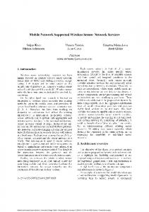
TMECH-06-2011-1730 this FMSN has the potential to fulfill functions of negotiating in complex steel structures with narrow sections and high abrupt angle changes. Guo et al. [11] further analyzed the compliant mechanism of the FMSN, and developed strategies to optimize design parameters for corner negotiation and sensor attachment. Zhu et al. [12] investigated the damage detection performance of the FMSNs using a laboratory steel frame structure. In the laboratory experiments, the mobile sensor network is able to detect minor structural damage, illustrating a high detection accuracy enabled by the flexible deployment of FMSNs. This paper investigates the field performance of the FMSNs with a space frame pedestrian bridge on Georgia Tech campus. Multiple FMSNs are wirelessly commanded to navigate to different sections of the steel bridge, for measuring structural vibrations at high spatial resolution. Using a small number of FMSNs, detailed modal characteristics of the bridge are identified. A finite element (FE) model for this bridge is constructed and successfully updated based on the modal characteristics extracted from FMSN data. The rest of the paper is organized as follows. Section II introduces the design of an FMSN. Section III describes the space frame bridge and experiment setup, and the experimental modal identification results are given in Section IV.. Section V presents the FE model updating process. Finally, a summary and discussion are provided. II. DESIGN OF THE FLEXURE-BASED MOBILE SENSING NODE A. General description of an FMSN Figure 1 shows the picture of an FMSN developed for this study [10-12]. The FMSN consists of three substructures: two 2-wheel cars and a compliant connection beam. Each 2-wheel car contains a body frame, two motorized wheels, batteries, a wireless sensing unit as described in [13], as well as associated sensors. The compliant connection beam is made of spring steel, with an accelerometer mounted in the middle. The dimensions and the weight of the FMSN are listed in Table I. Operating with Signal conditioning module

IR sensor

Wireless sensing unit

Compliant beam

Wireless sensing unit

Hall effect sensor

Accelerometer

IR sensor

Magnets layer

Hall effect sensor Wheel

Tape

Figure 1. Picture of the FMSN

IR sensor

2 TABLE I. PHYSICAL PARAMETERS OF THE FMSN Parameter Length Width Height Weight

Value 0.229m (9 in) 0.152m (6 in) 0.091m (3.6 in) 1 kg (2.2 lbs)

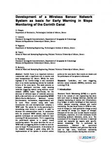
onboard batteries and communicating wirelessly, no external cable for power or communication is required. The wireless sensing unit serves as the “brain” of each FMSN, and performs various tasks such as sampling analog sensor signals, processing sensor data, motor control, and wireless communication with a central server or its peers. In order to capture low-amplitude vibrations, e.g. due to ambient excitation, a low-noise high-gain signal conditioning module [14] is equipped on each FMSN. This module (with amplification gain adjustable to ×2, ×20, ×200, or ×2,000) consists of a high-pass RC filter and a low-pass 4th-order Bessel filter with cutoff frequencies of 0.014Hz and 25Hz respectively. The wheels of the FMSN are enveloped by thin magnets (with magnetization axes arranged alternately pointing towards and away from the wheel center) to provide attraction for climbing on ferromagnetic structures. A Hall-effect sensor is fixed above each magnet wheel for measuring the periodical change of the magnetic flux as the wheel rotates, which provides wheel velocity feedback for real-time control. For the FMSN to move (forward or backward) safely on the underlying structural surface, infrared (IR) sensors are placed at both sides of the front and rear 2-wheel cars for surface boundary detection. When an IR sensor moves outside the surface boundary, changes can be captured from a reduced strength of the reflected IR signal, so that the movement direction can be immediately corrected through motor control. B. Flexure-based design One distinctive feature of the FMSN is the flexure-based design. Compared to a traditional rigid body design, the compliant/flexural connecting beam offers advantages for sharp corner negotiation and accurate acceleration measurement by firmly attaching the accelerometer onto the structural surface. During corner negotiation, when a rigid body design is adopted, the distance between front and rear axles has to remain constant. In order to avoid undesired slippage between each wheel and the structural surface, a complicated feedback control scheme will be necessary to precisely control individual wheel speed. On the other hand, using a flexure-based design, the axle distance can change passively and naturally, while the front and rear wheels simply move at a constant speed and do not suffer any slippage. Figure 2 shows the FMSN negotiating over the beam-column corner of a laboratory steel frame, when the front and rear wheels move at the same constant speed. The traces of the wheels are captured by image processing techniques and marked in the figure. With the flexure-based design, the FMSN can firmly attach the accelerometer onto the structural surface. The attachment is achieved by commanding the two cars move towards each other

TMECH-06-2011-1730

Figure 2. Corner negotiation on a laboratory structure.

(a)

3

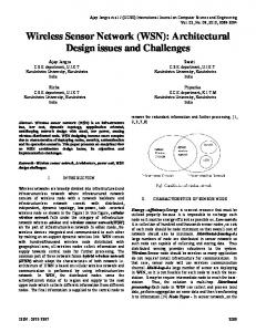
Figure 4. Picture of the space frame bridge on Georgia Tech campus.

measurement configurations are adopted by the FMSNs. As shown in Figure 5(a), each configuration consists of four measurement locations. Locations at south side of the frame are marked with letter ‘S’, and locations at north side are marked with letter ‘N’. The measurement configurations for the FMSNs do not contain locations 4S and 4N, where static wireless sensing nodes are mounted as reference nodes for assembling the mode shapes of the entire bridge. Wirelessly controlled by a laptop server located on the floor level at one side of the bridge Figure 5(b), the FMSNs start from the inclined members at one side of the bridge (Figure 6a), and then move to the 1st TABLE II. DIMENSIONS OF THE STEEL BRIDGE

(b) (c) Figure 3. Sensor attachment: (a) above a horizontal beam; (b) under a horizontal beam; (c) on a vertical column.

to bend the center of compliant beam towards the structural surface. In addition, small magnet pieces are arranged around the center of the beam to further assist the attachment. After measurement is finished, the two cars move in opposite directions to straighten the beam and lift the accelerometer away from the structural surface. After the accelerometer is lifted, the FMSN resumes its mobility and moves to next location for other measurement. As shown in Figure 3, the accelerometer can be attached along different directions (e.g. down, up, or horizontally) towards the structural surface. Detailed mechanical analysis of the flexure-based design can be found in [11]. III. BRIDGE TESTBED DESCRIPTION AND EXPERIMENTAL SETUP The pedestrian steel bridge testbed (Figure 4) is located on Georgia Tech campus, connecting the Manufacturing Research Center (MARC) with the Manufacturing Related Disciplines Complex (MRDC). The bridge consists of eleven chord units. Diagonal tension bars are deployed in two vertical side planes and the top horizontal planes, and each floor unit contains a diagonal bracing tube. Hinge connections are designed at the supports on the MRDC side, and roller connections at the MARC side. Key dimensions of the bridge are listed in Table II. In the field testing, four FMSNs are deployed for navigating on the top plane of the frame. It is first verified that each FMSN can travel through the bridge span of 30.2m (99 ft) in about five minutes, without stop. Onboard lithium-ion batteries can sustain the FMSN operation for about 4 hr. A total of five

Dimension

Value

Length Width Height Concrete floor slab thickness

Cross section and thickness of square tubes

11 × 2.74m = 30.2m (99 ft) 2.13m (7 ft) 2.74m (9 ft) 0.139 m (5.5 in)

Top-plane longitudinal

0.152 m × 0.152 m × 0.0080 m (6 in × 6 in × 5/16 in)

Bottom-plane longitudinal

0.152 m × 0.152 m × 0.0095 m (6 in × 6 in × 3/8 in) 0.152 m × 0.152 m × 0.0064 m (6 in × 6 in × 1/4 in)

Others

Static wireless sensor 4th Configuration 10S Mobile sensor rd 9S 3 Configuration 8S Hammer excitation 10 N 7S nd 9N 6S 2 Configuration N 2S

1S 1N

3N

2N

5S

4S

1st Configuration 3S

4N

6N

5N

7N

11 S 11N

8

5th Configuration

(a) Wireless server

Accelerometer

(b)

(c)

Figure 5. Experimental setup for the bridge testing: (a) 3D illustration of five measurement configurations for the FMSNs; (b) a laptop as the wireless server; (c) an FMSN attaches an accelerometer onto the structural surface.

TMECH-06-2011-1730

4

Static wireless sensor Hammer excitation

1S 1N

3N

2N

5S

4S

3S

2S

4N

5N

8S

7S

6S 6N

8N

7N

10 S

9S 9N

11 S 11N

10 N

Figure 7. Experimental setup for the testing with static wireless sensors. (a)

Hammer impact record Force (N)

15000 10000 5000 0 0.02 0.04 0.06 0.08 0.1 Time (s)

(a)

(b)

Figure 8. Hammer impact test: (a) a hammer impact being applied; (b) example hammer impact record.

IV. EXPERIMENTAL RESULTS This section begins with presenting the measurement and modal identification results from the hammer impact data,

A. Hammer impact test Hammer impact test with the FMSNs is first conducted. Individual hammer impact is applied at two locations on the floor, which are directly below locations 4S and 8N in Figure 8(a). After the four FMSNs arrive at each configuration, hammer impact is first applied at the floor below 4S for data collection, and then another impact is applied below 8N. Figure 8(a) shows the picture of a hammer impact being applied with a 3-lb hammer manufactured by PCB Piezotronics. The impact head allows for different tips to be affixed to the end, for varying the impact frequency range. A soft plastic tip is used in this study, for generating flat impact spectra up to a few hundred Hertz. The impact force is recorded by a cabled DAQ system (National Instruments 9235) (Figure 8b). During hammer impact test, the amplification gain of the signal conditioning module in the FMSNs is set to ×20 for Time history at 5S

FRF function at 5S 3

Amplitude

0.01

0

-0.01 0

5 10 Time (s)

2 1 0 0

15

Time history at 9N

10

3

0

-0.01 0

5 Frequency (Hz)

FRF function at 9N

0.01 Amplitude

measurement configuration (Figure 6b). After finishing the measurement at the 1st configuration, the FMSNs move to the 2nd configuration, and so on, until they finish measurement at the 5th configuration. At every measurement configuration, each FMSN attaches an accelerometer onto the structural surface, and measures structural vibrations along the vertical direction (Figure 5c). The accelerometer used in this study is a single-axis accelerometer (Silicon Designs 2260-010) with a frequency bandwidth of 0-300 Hz. The measurement range is ±2g, and the sensitivity is 1V/g, where ‘g’ is the gravitational acceleration. For the wireless data transmission from the FMSNs to the server, a simple star topology network is adopted. Acceleration data are temporarily stored onboard by each FMSN, and then sequentially collected by the server. Detailed information about the wireless network operation can be found in [13]. For comparison, another set of instrumentation is conducted entirely with static wireless sensors. Static sensors are installed at the measurement locations on the top plane of the bridge frame (Figure 7). Narada wireless sensing units, developed by researchers at the University of Michigan [15-17], are used in the static sensor instrumentation. The reliable performance of the Narada system has been validated in a number of previous studies. Modal analysis results using the static sensor data serve as a baseline for the FMSN data. The same Silicon Designs 2260-010 accelerometers are used in the static sensor instrumentation for measuring vertical vibrations.

followed by the modal identification results using ambient vibration data. Finally, the modal analysis results from FMSN data and static sensor data are compared.

Acceleration (g)

Figure 6. Pictures of four FMSNs navigating on the space frame bridge: (a) the FMSNs start from the incline members; (b) the FMSNs arrive at the 1st measurement configuration.

Acceleration (g)

(b)

5 10 Time (s)

15

2 1 0 0

5 Frequency (Hz)

10

Figure 9. Example vibration records and corresponding FRF function when the hammer impact is applied on the floor below location 4S.

TMECH-06-2011-1730 FRF function at 5S

0.01 Amplitude

Acceleration (g)

Time history at 5S

0

-0.01 0

5 10 Time (s)

3

A  Σ n1/ 2 U Tn H(1)Vn Σ n1/ 2

2

B  Σ1n/ 2 VnT Em

1

C  E Un Σ

0 0

15

T n

5 Frequency (Hz)

10

FRF function at 9N 3

Amplitude

Acceleration (g)

Time history at 9N 0.01

0

-0.01 0

5 10 Time (s)

5

15

2 1 0 0

5 Frequency (Hz)

10

Figure 10. Example vibration records and corresponding FRF function when the hammer impact is applied on the floor below location 8N.

acceleration measurement. The sampling rate is set to 1,000Hz. Figure 9 presents example acceleration time histories recorded at locations 5S and 9N, as well as the corresponding frequency response function (FRF) plots when the hammer impact is applied on the floor below location 4S. Figure 10 shows some example acceleration time histories and corresponding FRF plots, when the impact is applied below location 8N. The eigensystem realization algorithm (ERA) [18] is applied to the impulse FRF function for extracting modal characteristics at each configuration. In the ERA algorithm, the Hankel matrix H is formed as

y (k  1)  y (k  s  1)   y (k )  y (k  1)     H(k  1)          y (k  s  r  2) y (k  r  1)

where ETn = [I 0] and ETm = [I 0]. The estimated modes Γ can be obtained by ~~ (5) Γ  CΦ ~ ~ where Φ contains the eigenvectors of matrix A . In order to obtain reliable modal results and alleviate the noise effect, for configurations 1~3 in Figure 5(a), the modal characteristics are extracted using FMSN data when hammer impact is applied below location 4S. For configurations 4 and 5, the modal characteristics are extracted using FMSN data when hammer impact is applied below location 8N. The mode shapes of the entire bridge are assembled through the reference nodes with two static wireless sensors (Figure 5a). Figure 11 shows the first three assembled mode shapes. Note that because both the hammer impact and the accelerometer measurement are along the vertical direction, the modal testing is only able to capture mode shapes with relatively strong vertical components. Similarly, hammer impact test is conducted with static sensors measuring vibrations at all locations. Figure 12 presents the first Mode 1: f = 4.63Hz 30

0 0

30

25

(1)

25 20

15

15

10 2

10

5

0

2

30 25 20 15 10

(2)

5

0

Figure 11. First three mode shapes of the bridge extracted from FMSN data with hammer impact excitation.

Mode 2: f = 6.93Hz

Mode 1: f = 4.64Hz

(3)

where n is a diagonal matrix with non-zero singular values. In practice, using experimental data, other singular values will not appear as exactly zero, but instead as relatively small numbers along the diagonal of , which correspond to spurious noise modes. The rows and columns associated with the noise modes are then eliminated to form condensed matrices n , Un , and Vn. The estimated state-space matrices for the discrete-time system model are then calculated as

5

0

Mode 3: f = 10.54Hz

2

where matrices U and V contain left and right singular vectors of H(0), respectively;  is a diagonal matrix with singular values. Theoretically, matrix  with rank of n can be express as

Σ Σ n 0

Mode 2: f = 6.97Hz

20

where y(k) is the impulse response vector at the k-th discrete time step; r and s are integers that determine the Hankel matrix dimension. Singular value decomposition is performed on matrix H(0): H(0) = UVT

(4)

1/ 2 n

30

30

25

25

20

20

15

15

10

10 2

0

5

2

5

0

Mode 3: f = 10.51Hz 30 25 20 15 10 2

0

5

Figure 12. First three mode shapes of the bridge extracted from static sensor data with hammer impact excitation.

TMECH-06-2011-1730 three mode shapes extracted from the static sensor data. Comparison between Figure 11 and Figure 12 shows that the natural frequencies and mode shapes extracted from FMSN data and static sensor data are very close. B. Ambient vibration test During the ambient vibration test, 10 minutes of continuous acceleration data are collected for each mobile measurement configuration. The amplification gain of the signal conditioning module is set to ×200 during ambient vibration test, and the sampling rate is set to 100Hz. Figure 13 presents example ambient vibration time histories recorded at locations 5S and 9N, as well as the corresponding power spectral density (PSD) plots. The natural excitation technique (NExT) [19, 20] is applied to the FMSN data to extract modal characteristics at each configuration. In the NExT method, it is assumed that the excitation and response are stationary random processes. The dynamics equation for a multi-degree-of-freedom system is written as

Mx  t   Cx  t   Kx  t   f  t 

(6)

where M, C, and K represent mass, damping, and stiffness matrices of the system, respectively; x(t) is displacement vector random process; and f(t) is excitation vector random process. Multiplying equation (6) by a reference scalar response process xi(s), and taking the expected value of the equation gives:

ME x  t  xi  s   CE x  t  xi  s   KE x  t  xi  s 

(7)

 E f  t  xi  s 

where E{} represents expectation. Assuming that the vector random processes x(t), x(t ) and x(t ) are weakly stationary,

6

the excitation (at time t). Equation (8) can then be simplified as [21]:

MR xxi    CR xxi    KR xxi    0

(9)

Therefore, the cross correlation function satisfies the dynamics equation describing free vibration, and can be used as input to the ERA algorithm for modal identification. The procedure is performed to the FMSN data from ambient vibration. Similar as the hammer data analysis, the mode shapes for the entire bridge are assembled through the two reference nodes with static wireless sensors. Figure 14 shows the first three mode shapes of the bridge extracted from ambient vibration data collected by the FMSNs. C. Modal analysis comparison The natural frequencies extracted from hammer impact test and ambient vibration data are summarized in Table III. The frequency differences extracted from FMSN data and static sensor data are very small. To evaluate the differences in mode shapes, the modes extracted from static sensor data are used as the reference modes, and the modal assurance criterion (MAC) value is calculated for mode shapes extracted from FMSN data:

MACi 

φ

φ T M ,i

T M ,i

φ M ,i

φ S ,i

φ



2

T S ,i

φ S ,i

(10)



where φ M ,i and φ S ,i denote the i-th mode shape extracted from FMSN data and static sensor data, respectively; MACi represents the i-th MAC value between the i-th mode shapes. Note that if the mode shapes φ M ,i and φ S ,i are close to Mode 2: f = 6.92Hz

Mode 1: f = 4.67Hz

equation (7) can be written as 30

30

MR xxi    CR xxi    KR xxi    Rfxi  

25

25

(8)

20

20

15

15

where R represents the cross correlation function, and   t  s . With   0 , the system response (at time s) are uncorrelated to 2

x 10

0

5

2

5

0

Mode 3: f = 10.28Hz

PSD at 5S -60

30 25

0

-2 0

100

-3

2

x 10

200 300 Time (s)

400

500

15

-80

10 2

Time history at 9N

5 Frequency (Hz)

10

PSD at 9N

100

200 300 Time (s)

400

500

0

5

Figure 14. First three mode shapes of the bridge extracted from ambient vibration data collected by the FMSNs. TABLE III. COMPARISON OF MODAL CHARACTERISTICS EXTRACTED FROM FMSN DATA AND STATIC SENSOR DATA

-70

0

-2 0

20

-100 0

PSD (dB)

Acceleration (g)

Time history at 5S PSD (dB)

Acceleration (g)

-3

10

10 2

-80 -90 -100 0

Mode No. 5 Frequency (Hz)

10

Figure 13. Example ambient vibration records and corresponding power spectral density (PSD) plots.

1 2 3

Natural frequencies (Hz) Mobile data (hammer) 4.63 6.97 10.54

Mobile data (ambient) 4.67 6.92 10.28

MAC values for FMSN data

Static data Hammer (hammer) 4.64 0.99 6.93 0.99 10.51 0.97

Ambient 0.99 0.96 0.96

TMECH-06-2011-1730 each other, MACi should be close to 1. The MAC values shown in Table III are all greater than 0.95. Therefore, it can be concluded that the mobile sensing system is capable of providing consistent and reliable sensor data with high spatial resolution. V. FINITE ELEMENT MODEL UPDATING

B. Model updating Important parameters of the bridge model are selected for FE model updating. The parameters typically include material properties and support conditions [23, 24]. For support conditions, ideal hinges or rollers are usually used in structural design and analysis, but do not exist in reality. To describe realistic support conditions, the hinge support at MRDC side is replaced by a rigid link in longitudinal direction, and springs in transverse and vertical directions. Meanwhile, the roller support at MARC side is replaced by springs in transverse and vertical directions (Figure 15). In this study, ten parameters of the bridge model are chosen for updating, including density, elastic modulus, spring stiffness, etc. Table IV summarizes the updating parameters, as well as their initial values determined from design drawings and engineering judgment.

MARC side

z y

x

MRDC side

(a) ky1

ky2

kz1

(b)

TABLE IV. SELECTED PARAMETERS FOR MODEL UPDATING Updating parameters

kz2

(c)

Figure 15. FE model for the steel bridge: (a) 3D view of the bridge model; (b) support condition at MRDC side for model updating; (c) support condition at MARC side for model updating.

Initial value Optimal value

3

Concrete Slab Steel

A. Base model for finite element updating A FE model of the bridge is built in the OpenSees (Open System for Earthquake Engineering Simulation [22]) platform. All steel frame members are modeled as elastic beam-column elements, and steel tension bars on the side and top planes are modeled as 3D truss elements. In structural design practice, concrete slab is usually considered as dead load with no contribution to structural stiffness. However, the concrete slab in this structure is connected with the bottom-plane frame members by sheer studs, through which bending moment can be transferred. Therefore, for accurate dynamic modeling, the concrete floor slab is modeled as shell elements that share FE nodes with the bottom-plane frame members.

7

Support

2.48×103 2.07×1010 1.4×10-1 7.87×103 2.0×1011 2.0×1011 3.50×104 8.76×104 3.50×104 8.76×104

Density (kg/m ) Elastic modulus (N/m2) Thickness (m) Density (kg/m3) Elastic modulus Frame tubes ( N/m2) Tension bars Transverse ky1 (kN/m) Vertical kz1 (kN/m) Transverse ky2 (kN/m) Vertical kz2 (kN/m)

2.64×103 1.65×1010 1.4×10-1 8.26×103 1.9×1011 2.0×1011 2.45×104 1.40×105 2.45×104 1.40×105

Using MATLAB optimization toolbox [25], an interior-point optimization procedure is performed for minimizing the difference between three experimental natural frequencies extracted from FMSN data and corresponding frequencies provided by FE model:

 f  f M ,i minimize  FE ,i  f M ,i i 

  

2

(11)

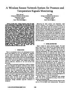
where f FE ,i denotes the i-th natural frequency provided by the FE model, and f M ,i denotes the frequency extracted from FMSN data during the hammer impact test (as listed in Table III). The final updated optimal values are shown in Table IV. C. Comparison between simulation and experiments Using the updated parameter values, first five natural frequencies and mode shapes from the FE model are shown in Figure 16. Plots in the left column are the mode shapes of the bridge model in 3D view. Plots in the right column illustrate only the vertical components of the mode shapes at the top-plane nodes, for direct comparison with experimental results. For each mode shape, the Z/Y ratio equals the maximum Z-direction magnitude in the mode shape vector divided by the maximum Y-direction magnitude. Mode shapes with large and moderate Z/Y ratios have relatively strong vertical direction components, which make them easily captured by the single-axis accelerometer used in the FMSNs (for measuring vertical vibration). It can be seen that the Vertical-1 mode from the FE model corresponds to Mode-1 extracted from experimental data (described in Section IV), the Torsional-1 mode corresponds to Mode-2, and Vertical-2 corresponds to Mode-3. On the contrary, mode shapes with small Z/Y ratios (i.e. Lateral-1 and Lateral-2) have trivial vertical direction components. These two mode shapes are not reliably captured by the FMSN measurements during the modal testing. Table V compares the modal characteristics extracted from the FMSN data (during hammer impact test) with those from FE simulation. The errors for all three natural frequencies are below 5%. The MAC values between the experimental and simulated mode shapes are very close to 1 for Mode-1 and Mode-2, and about 0.8 for Mode-3.

TMECH-06-2011-1730

Lateral-1

f = 4.07Hz

Z/Y=0.17 30 25 20 15 10 2

Vertical-1

f= 4.64Hz

5

0

Z/Y=10.64 30 25 20 15 10 2

Torsional-1

f= 6.65 Hz

0

5

Z/Y=0.45 30 25 20 15 10 2

Lateral-2

f= 8.77Hz

0

5

Z/Y=0.20

8

extracted from the FMSN data are compared with those extracted from static sensor data. It is shown the mobile sensing system is capable of providing consistent and reliable measurement. In addition, an FE model for the steel bridge is built in OpenSees and updated based upon the modal characteristics extracted from FMSN data. The updated FE model provides similar modal characteristics as the experimental results. Future research will improve the FMSN design for navigating on more complicated real-world structures. For example, work is in progress developing a mobile sensing node that can make left or right turns. More agile mobile sensing nodes will conveniently provide more vibration measurement locations along different directions. Besides, current FMSN can only move on relatively smooth structural surface. The ability of navigating over difficult obstacles, such as large bolts and rivets, need to be investigated in future research. In addition, a camera may be equipped on the FMSN, and localization and mapping algorithms can be embedded in the node. Combining locomotion data with information from structural design drawings, the FMSN may be able to locate itself on the structure.

30 25 20 15

ACKNOWLEDGEMENT

10 2

Vertical-2

f= 10.94 Hz

0

5

Z/Y=10.73 30 25 20

This research is partially sponsored by the National Science Foundation, under grant number CMMI-0928095. In addition, the authors would like to thank the help with the field testing provided by a number of graduate research assistants at Georgia Tech, including Chunxu Qu, Chia-Hung Fang, and Xiaohua Yi.

15 10 2

0

5

REFERENCES

Figure 16. First five mode shapes of the FE model.

[1]

TABLE V. COMPARISON OF MODAL CHARACTERISTICS EXTRACTED FROM FMSN DATA AND FE SIMULATION

[2]

Natural frequencies (Hz) FMSN data FE simulation (hammer impact) 4.63 (Mode-1) 4.64 (Vertical-1) 6.97 (Mode-2) 6.65 (Torsional-1) 10.54 (Mode-3) 10.94 (Vertical-2)

Error

MAC values

0.02% 4.15% 4.07%

0.99 0.97 0.78

[3]

[4]

[5]

VI. CONCLUSION Exploratory work harnessing mobile sensor network for civil structure monitoring is presented in this paper. Four FMSN nodes navigate autonomously to different sections of a steel bridge, for measuring vibrations under hammer impact and ambient excitations. Modal analysis is successfully conducted using the FMSN data. To validate the mobile sensing performance, a static wireless sensor network is installed on the bridge for measuring structural vibrations under hammer impact. The natural frequencies and corresponding mode shapes

[6]

[7]

[8]

[9]

J. P. Lynch and K. J. Loh, "A summary review of wireless sensors and sensor networks for structural health monitoring," The Shock and Vibration Digest, vol. 38, pp. 91-128, 2006. I. F. Akyildiz, W. Su, Y. Sankarasubramaniam, and E. Cayirci, "A survey on sensor networks," Communications Magazine, IEEE, vol. 40, pp. 102-114, 2002. F. Tache, W. Fischer, G. Caprari, R. Siegwart, R. Moser, and F. Mondada, "Magnebike: A magnetic wheeled robot with high mobility for inspecting complex-shaped structures," Journal of Field Robotics, vol. 26, pp. 453-476, 2009. C. Choi, B. Park, and S. Jung, "The design and analysis of a feeder pipe inspection robot with an automatic pipe tracking system," Mechatronics, IEEE/ASME Transactions on, vol. 15, pp. 736-745, 2010. M. P. Murphy and M. Sitti, "Waalbot: an agile small-scale wall-climbing robot utilizing dry elastomer adhesives," Mechatronics, IEEE/ASME Transactions on, vol. 12, pp. 330-338, 2007. W. R. Provancher, S. I. Jensen-Segal, and M. A. Fehlberg, "ROCR: an energy-efficient dynamic wall-climbing robot," Mechatronics, IEEE/ASME Transactions on, vol. 16, pp. 897-906, 2011. D. R. Huston, B. Esser, G. Gaida, S. W. Arms, and C. P. Townsend, "Wireless inspection of structures aided by robots," Proceedings of SPIE, Health Monitoring and Management of Civil Infrastructure Systems, Newport Beach, CA, 2001. P. G. Backes, Y. Bar-Cohen, and B. Joffe, "The multifunction automated crawling system (MACS)," Proceedings of the 1997 IEEE International Conference on Robotics and Automation, Albuquerque, New Mexico, 1997. M. Todd, D. Mascarenas, E. Flynn, T. Rosing, B. Lee, D. Musiani, S. Dasgupta, S. Kpotufe, D. Hsu, R. Gupta, G. Park, T. Overly, M. Nothnagel, and C. Farrar, "A different approach to sensor networking for

TMECH-06-2011-1730

[10]

[11]

[12]

[13]

[14]

[15]

[16]

[17]

[18]

[19]

[20]

[21] [22]

[23]

[24]

[25]

SHM: remote powering and interrogation with unmanned aerial vehicles," Proceedings of the 6th International Workshop on Structural Health Monitoring, Stanford, CA, 2007. K.-M. Lee, Y. Wang, D. Zhu, J. Guo, and X. Yi, "Flexure-based mechatronic mobile sensors for structure damage detection," Proceedings of the 7th International Workshop on Structural Health Monitoring, Stanford, CA, USA, 2009. J. Guo, K.-M. Lee, D. Zhu, X. Yi, and Y. Wang, "Large-deformation analysis and experimental validation of a flexure-based mobile sensor node," IEEE/ASME Transactions on Mechatronics, 10.1109/TMECH.2011.2107579, 2011. D. Zhu, X. Yi, Y. Wang, K.-M. Lee, and J. Guo, "A mobile sensing system for structural health monitoring: design and validation," Smart Materials and Structures, vol. 19, p. 055011, 2010. Y. Wang, J. P. Lynch, and K. H. Law, "A wireless structural health monitoring system with multithreaded sensing devices: design and validation," Structure and Infrastructure Engineering, vol. 3, pp. 103-120, 2007. Y. Q. Ni, B. Li, K. H. Lam, D. Zhu, Y. Wang, J. P. Lynch, and K. H. Law, "In-construction vibration monitoring of a super-tall structure using a long-range wireless sensing system," Smart Structures and Systems, vol. 7, pp. 83-102, 2011. A. T. Zimmerman, M. Shiraishi, R. A. Swartz, and J. P. Lynch, "Automated modal parameter estimation by parallel processing within wireless monitoring systems," Journal of Infrastructure Systems, vol. 14, pp. 102-113, 2008. R. A. Swartz, D. Jung, J. P. Lynch, Y. Wang, D. Shi, and M. P. Flynn, "Design of a wireless sensor for scalable distributed in-network computation in a structural health monitoring system," Proceedings of the 5th International Workshop on Structural Health Monitoring, Stanford, CA, 2005. R. A. Swartz and J. P. Lynch, "Strategic network utilization in a wireless structural control system for seismically excited structures," Journal of Structural Engineering, vol. 135, pp. 597-608, 2009. J. N. Juang and R. S. Pappa, "An eigensystem realization algorithm for modal parameter identification and modal reduction," Journal of Guidance Control and Dynamics, vol. 8, pp. 620-627, 1985. J. M. Caicedo, S. J. Dyke, and E. A. Johnson, "Natural excitation technique and eigensystem realization algorithm for Phase I of the IASC-ASCE benchmark problem: simulated data," Journal of Engineering Mechanics, vol. 130, pp. 49-60, 2004. C. R. Farrar and G. H. James, "System identification from ambient vibration measurements on a bridge," Journal of Sound and Vibration, vol. 205, pp. 1-18, 1997. J. S. Bendat and A. G. Piersol, Random data: Analysis and measurement procedure. New York: Wiley, 2000. F. McKenna, OpenSees: Open System for Earthquake Engineering Simulation (web page and software), http://opensees.berkeley.edu/. Last accessed: October 27, 2011. A. E. Aktan, N. Catbas, A. Turer, and Z. Zhang, "Structural identification: Analytical aspects," Journal of Structural Engineering, vol. 124, pp. 817-829, 2002. F. N. Catbas, S. K. Ciloglu, O. Hasancebi, K. Grimmelsman, and A. E. Aktan, "Limitations in structural identification of large constructed structures," Journal of Structural Engineering, vol. 133, pp. 1051-1066, 2007. MathWorks Inc., Optimization ToolboxTM User's Guide, R2011b ed. Natick, MA: MathWorks Inc., 2011.

9