Worst-Case Optimal Priority Queues via Extended Regular Counters

Worst-Case Optimal Priority Queues via Extended Regular Counters Amr Elmasry and Jyrki Katajainen

arXiv:1112.0993v1 [cs.DS] 5 Dec 2011

Department of Computer Science, University of Copenhagen, Denmark

Abstract. We consider the classical problem of representing a collection of priority queues under the operations find -min, insert, decrease, meld , delete, and delete-min. In the comparison-based model, if the first four operations are to be supported in constant time, the last two operations must take at least logarithmic time. Brodal showed that his worst-case efficient priority queues achieve these worst-case bounds. Unfortunately, this data structure is involved and the time bounds hide large constants. We describe a new variant of the worst-case efficient priority queues that relies on extended regular counters and provides the same asymptotic time and space bounds as the original. Due to the conceptual separation of the operations on regular counters and all other operations, our data structure is simpler and easier to describe and understand. Also, the constants in the time and space bounds are smaller. In addition, we give an implementation of our structure on a pointer machine. For our pointermachine implementation, decrease and meld are asymptotically slower and require O(lg lg n) worst-case time, where n denotes the number of elements stored in the resulting priority queue.

1

Introduction

A priority queue is a fundamental data structure that maintains a set of elements and supports the operations find -min, insert, decrease, delete, delete-min, and meld . In the comparison-based model, from the Ω(n lg n) lower bound for sorting it follows that, if insert can be performed in o(lg n) time, delete-min must take Ω(lg n) time. Also, if meld can be performed in o(n) time, delete-min must take Ω(lg n) time [2]. In addition, if find -min can be performed in constant time, delete would not be asymptotically faster than delete-min. Based on these observations, a priority queue is said to provide optimal time bounds if it can support find -min, insert, decrease, and meld in constant time; and delete and delete-min in O(lg n) time, where n denotes the number of elements stored. After the introduction of binary heaps [16], which are not optimal with respect to all priority-queue operations, an important turning point was when Fredman and Tarjan introduced Fibonacci heaps [11]. Fibonacci heaps provide optimal time bounds for all standard operations in the amortized sense. Driscoll et al. [6] introduced run-relaxed heaps, which have optimal time bounds for all operations in the worst case, except for meld . Later, Kaplan and Tarjan [14] (see also [12]) introduced fat heaps, which guarantee the same worst-case bounds as

run-relaxed heaps. On the other side, Brodal [2] introduced meldable priority queues, which provide the optimal worst-case time bounds for all operations, except for decrease. Later, by introducing several innovative ideas, Brodal [3] was able to achieve the worst-case optimal time bounds for all operations. Though deep and involved, Brodal’s data structure is complicated and should just be taken as a proof of existence. Kaplan et al. [12] said the following about Brodal’s construction: “This data structure is very complicated however, much more complicated than Fibonacci heaps and the other meldable heap data structures”. To appreciate the conceptual simplicity of our construction, we urge the reader to scan through Brodal’s paper [3]. On the other side, we admit that while trying to simplify Brodal’s construction, we had to stick with many of his innovative ideas. We emphasize that in this paper we are mainly interested in the theoretical performance of the priority queues discussed. However, some of our ideas may be of practical value. Most priority queues with worst-case constant decrease, including the one to be presented by us, rely on the concept of violation reductions. A violation is a node that may, but not necessarily, violate the heap order by being smaller than its parent. When the number of violations becomes high, a violation reduction is performed in constant time to reduce the number of violations. A numeral system is a notation for representing numbers in a consistent manner using symbols—digits. In addition, operations on these numbers, as increments and decrements of a given digit, must obey the rules governing the numeral system. There is a connection between numeral systems and data-structural design [4, 15]. The idea is to relate the number of objects of a specific type in the data structure to the value of a digit. A representation of a number that is subject to increments and decrements of arbitrary digits can be called a counter. A regular counter [4] uses the digits {0, 1, 2} in the representation of a number and imposes the rule that between any two 2’s there must be a 0. Such a counter allows for increments (and also decrements, under the assumption that the digit being decreased was non-zero) of arbitrary digits with a constant number of digit changes per operation. For an integer b ≥ 2, an extended regular b-ary counter uses the digits {0, . . . , b, b+1} with the constraints that between any two (b+1)’s there is a digit other than b, and between any two 0’s there is a digit other than 1. An extended regular counter [4, 12] allows for increments and decrements of arbitrary digits with a constant number of digit changes per operation. Kaplan and Tarjan [14] (see also [12]) introduced fat heaps as a simplification of Brodal’s worst-case optimal priority queues, but these are not meldable in O(1) worst-case time. In fat heaps, an extended regular ternary counter is used to maintain the trees in each heap and an extended regular binary counter to maintain the violation nodes. In this paper, we describe yet another simplification of Brodal’s construction. One of the key ingredients in our construction is the utilization of extended regular binary counters. Throughout our explanation of the data structure, in contrary to [3], we distinguish between the operations of the numeral system and other priority-queue operations. Our motives for writing this paper were the following. 2

Table 1. The best-known worst-case comparison complexity of different priority-queue operations. The worst-case performance of delete is the same as that of delete-min. Using ’–’ indicates that the operation is not supported optimally. Data structure Multipartite priority queues [7] Two-tier relaxed heaps [8] Meldable priority queues [9] Optimal priority queues [this paper]

find -min O(1) O(1) O(1) O(1)

insert decrease meld delete-min O(1) – – lg n + O(1) O(1) O(1) – lg n + O(lg lg n) O(1) – O(1) 2 lg n + O(1) O(1) O(1) O(1) ≈ 70 lg n

1. We simplify Brodal’s construction and devise a priority queue that provides optimal worst-case bounds for all operations (§2 and §3). The gap between the description complexity of worst-case optimal priority queues and binary heaps [16] is huge. One of our motivations was to narrow this gap. 2. We describe a strikingly simple implementation of the extended regular counters (§4). In spite of their importance for many applications, the existing descriptions [4, 12] for such implementations are sketchy and incomplete. 3. With this paper, we complete our research program on the comparison complexity of priority-queue operations. All the obtained results are summarized in Table 1. Elsewhere, it has been documented that, in practice, worst-case efficient priority queues are often outperformed by simpler non-optimal priority queues. Due to the involved constant factors in the number of element comparisons, this is particularly true if one aims at developing priority queues that achieve optimal time bounds for all the standard operations. It is a long-standing open issue how to implement a heap on a pointer machine such that all operations are performed in optimal time bounds. A Fibonacci heap is known to achieve the optimal bounds in the amortized sense on a pointer machine [13], a fat heap in the worst case provided that meld is not supported [14], and the meldable heap in [2] provided that decrease is supported in O(lg n) time. In this paper, we offer a pointer-machine implementation for which decrease and meld are supported in O(lg lg n) worst-case time.

2

Description of the Data Structure

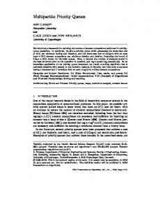
Let us begin with a high-level description of the data structure. The overall construction is similar to that used in [3]. However, the use of extended regular counters is new. In accordance, the rank rules, and hence the structure, are different from [3]. The set of violation-reduction routines are in turn new. For an illustration of the data structure, see Fig. 1. Each priority queue is composed of two multi-way trees T1 and T2 , with roots t1 and t2 respectively (T2 can be empty). The atomic components of the priority queues are nodes, each storing a single element. The rank of a node x, denoted rank (x), is an integer that is logarithmic in the size (number of nodes) of the subtree rooted at x. The rank of a subtree is the rank of its root. The trees T1 and T2 are heap ordered, 3

○ 1 r ○ 5

○ 1

t1

○ 2

t2

○ 2

○ 3 r

1111 0000 0000 1111 0000 1111 0000 1111 0000 1111

...

0000 ○ 4 1111 0000 1111

0000 1111 0000 1111 0000 1111 000 111 111 000 000 111 000 111 000 111

T1

T2 ○ 1 If t2 exists, rank (t1 ) < rank (t2 ). ○ 2 An extended regular binary counter is used to keep track of the children of each of t1 and t2 . ○ 3 For each node, including t1 and t2 , its rank sequence hd0 , d1 , . . . , d`−1 i must obey the following rules: for all i ∈ {0, 1, . . . , ` − 1} (i) di ≤ 3 and (ii) if di 6= 0, then di−1 6= 0 or di ≥ 2 or di+1 6= 0. ○ 4 Each node guards a list of violations; t1 guards two: one containing active violations and another containing inactive violations. ○ 5 The active violations of t1 are kept in a violation structure consisting of a resizable array, in which the rth entry refers to violations of rank r, and a doubly-linked list linking the entries of the array that have more than two violations. Fig. 1. Illustrating the data structure in an abstract form.

except for some violations; but, the element at t1 is the minimum among the elements of the priority queue. If t2 exists, the rank of t1 is less than that of t2 , i.e. rank (t1 ) < rank (t2 ). With each priority queue, a violation structure is maintained; an idea that has been used before in [3, 6, 12]. This structure is composed of a resizable array, called violation array, in which the rth entry refers to violations of rank r, and a doubly-linked list, which links the entries of the array that have more than two violations each. Similar to [3], each violation is guarded by a node that has a smaller element. Hence, when a minimum is deleted, not all the violations need to be considered as the new minimum candidates. To adjust this idea for our purpose, the violations guarded by t1 are divided into two groups: the so-called active violations are used to perform violation reductions, and the so-called inactive violations are violations whose ranks were larger than the size of the violation array at the time when the violation occurred. All the active violations guarded by t1 , besides being kept in a doubly-linked list, are also kept in the violation structure; all inactive violations are kept in a doubly-linked list. Any node x other than t1 only guards a single list of O(lg n) violations. These are the violations that took place while node x stored the minimum of its priority queue. Such violations must be tackled once the element associated with node x is deleted. In particular, in the whole data structure there can be up to O(n) violations, not O(lg n) violations as in run-relaxed heaps and fat heaps. 4

When a violation is introduced, there are two phases for handling it accordingly to whether the size of the violation array is as big as the largest rank or not. During the first phase, the following actions are taken. 1) The new violation is added to the list of inactive violations. 2) The violation array is extended by a constant number of entries. During the second phase, the following actions are taken. 1) The new violation is added to the list of active violations and to the violation structure. 2) A violation reduction is performed if possible. The children of a node are stored in a doubly-linked list in non-decreasing rank order. In addition to an element, each node stores its rank and six pointers pointing to: the left sibling, the right sibling (the parent if no right sibling exists), the last child (the rightmost child), the head of the guarded violation list, and the predecessor and the successor in the violation list where the node may be in. To decide whether the right-sibling pointer of a node x points to a sibling or a parent, we locate the node y pointed to by the right-sibling pointer of x and check if the last-child pointer of y points back to x. Next, we state the rank rules implying the structure of the multi-way trees: (a) The rank of a node is one more than the rank of its last child. The rank of a node that has no children is 0. (b) The rank sequence of a node specifies the multiplicities of the ranks of its children. If the rank sequence has a digit dr , the node has dr children of rank r. The rank sequences of t1 and t2 are maintained in a way that allows adding and removing an arbitrary subtree of a given rank in constant time. This is done by having the rank sequences of those nodes obey the rules of a numeral system that allows increments and decrements of arbitrary digits with a constant number of digit changes per operation. When we add a subtree or remove a subtree from below t1 or t2 , we also do the necessary actions to reestablish the constraints imposed by the numeral system. (c) Consider a node x that is not t1 , t2 , or a child of t1 or t2 . If the rank of x is r, there must exist at least one sibling of x whose rank is r − 1, r or r + 1. Note that this is a relaxation to the rules applied to the rank sequences of t1 and t2 , for which the same rule also applies [4]. In addition, the number of siblings having the same rank is upper bounded by at most three. Among the children of a node, there are consecutive subsequences of nodes with consecutive, and possibly equal, ranks. We call each maximal subsequence of such nodes a group. By our rank rules, a group has at least two members. The difference between the rank of a member of a group and that of another group is at least two, otherwise both constitute the same group. Lemma 1. The rank and the number of children of any node in our data structure is O(lg n), where n is the size of the priority queue. Proof. We prove by induction that the size of a subtree of rank r is at least Fr , where Fr is the rth Fibonacci number. The claim is clearly true for r ∈ {0, 1}. Consider a node x of rank r ≥ 2, and assume that the claim holds for all values smaller than r. The last child of x has rank r − 1. Our rank rules imply that 5

there is another child of rank at least r − 2. Using the induction hypothesis, the size of these two subtrees is at least Fr−1 and Fr−2 . Then, the size of the subtree rooted at x is at least Fr−1 + Fr−2 = Fr . Hence, the maximum rank of a node is 1.44 lg n. By the rank rules, every node has at most three children of the same rank. It follows that the number of children per node is O(lg n). t u Two trees of rank r can be joined by making the tree whose root has the larger value the last subtree of the other. The rank of the resulting tree is r + 1. Alternatively, a tree rooted at a node x of rank r + 1 can be split by detaching its last subtree. If the last group among the children of x now has one member, the subtree rooted at this member is also detached. The rank of x becomes one more than the rank of its current last child. In accordance, two or three trees result from a split; among them, one has rank r and another has rank r − 1, r, or r + 1. The join and split operations are used to maintain the constraints imposed by the numeral system. Note that one element comparison is performed with the join operation, while the split operation involves no element comparisons.

3

Priority-Queue Operations

One complication, also encountered in [3], is that not all violations can be recorded in the violation structure. The reason is that, after a meld , the violation array may be too small when the old t1 with the smaller rank becomes the new t1 of the melded priority queue. Assume that we have a violation array of size s associated with t1 . The priority queue may contain nodes of rank r ≥ s. Hence, violations of rank r cannot be recorded in the array. We denote the violations that are recorded in the violation array as active violations and those that are only in the violation list as inactive violations. Violation reductions are performed on active violations whenever possible. Throughout the lifetime of t1 , the array is incrementally extended by the upcoming priority-queue operations until its size reaches the largest rank. Once the array is large enough, no new inactive violations are created. Since each priority-queue operation can only create a constant number of violations, the number of inactive violations is O(lg n). The violation structures can be realized by letting each node have one pointer to its violation list, and two pointers to its predecessor and successor in the violation list where the node itself may be in. By maintaining all active violations of the same rank consecutively in the violation list of t1 , the violation array can just have a pointer to the first active violation of any particular rank. In connection with every decrease or meld , if T2 exists, a constant number of subtrees rooted at the children of t2 are removed from below t2 and added below t1 . Once rank (t1 ) ≥ rank (t2 ), the whole tree T2 is added below t1 . To be able to move all subtrees from below t2 and finish the job on time, we should always pick a subtree from below t2 whose rank equals the current rank of t1 . The priority queue operations aim at maintaining the following invariants: 1. The minimum is associated with t1 . 2. The second-smallest element is either stored at t2 , at one of the children of t1 , or at one of the violation nodes associated with t1 . 6

3. The number of entries in the violation list of a node is O(lg n), assuming that the priority queue that contains this node has n elements. We are now ready to describe how the priority-queue operations are realized. find -min(Q): Following the first invariant, the minimum is at t1 . insert(Q, x): A new node x is given with the value e. If e is smaller than the value of t1 , the roles of x and t1 are exchanged by swapping the two nodes. The node x is then added below t1 . meld (Q, Q0 ): This operation involves at most four trees T1 , T2 , T10 , and T20 , two for each priority queue; their roots are named correspondingly using lowercase letters. Assume without loss of generality that value(t1 ) ≤ value(t01 ). The tree T1 becomes the first tree of the melded priority queue. The violation array of t01 is dismissed. If T1 has the maximum rank, the other trees are added below t1 resulting in no second tree for the melded priority queue. Otherwise, the tree with the maximum rank among T10 , T2 , and T20 becomes the second tree of the melded priority queue. The remaining trees are added below the root of this tree, and the roots of the added trees are made violating. To keep the number of active violations within the threshold, two violation reductions are performed if possible. Finally, the regular counters that are no longer corresponding to roots are dismissed. decrease(Q, x, e): The element at node x is replaced by element e. If e is smaller than the element at t1 , the roles of x and t1 are exchanged by swapping the two nodes (but not their violation lists). If x is either t1 , t2 , or a child of t1 , stop. Otherwise, x is denoted violating and added to the violation structure of t1 ; if x was already violating, it is removed from the violation structure where it was in. To keep the number of active violations within the threshold, a violation reduction is performed if possible. delete-min(Q): By the first invariant, the minimum is at t1 . The node t2 and all the subtrees rooted at its children are added below t1 . This is accompanied with extending the violation array of T1 , and dismissing the regular counter of T2 . By the second invariant, the new minimum is now stored at one of the children or violation nodes of t1 . By Lemma 1 and the third invariant, the number of minimum candidates is O(lg n). Let x be the node with the new minimum. If x is among the violation nodes of t1 , a tree that has the same rank as x is removed from below t1 , its root is made violating, and is attached in place of the subtree rooted at x. If x is among the children of t1 , the tree rooted at x is removed from below t1 . The inactive violations of t1 are recorded in the violation array. The violations of x are also recorded in the array. The violation list of t1 is appended to that of x. The node t1 is then deleted and replaced by the node x. The old subtrees of x are added, one by one, below the new root. To keep the number of violations within the threshold, violation reductions are performed as many times as possible. By the third invariant, at most O(lg n) violation reductions are to be performed. delete(Q, x): The node x is swapped with t1 , which is then made violating. To remove the current root x, the same actions are performed as in delete-min.

7

In our description, we assume that it is possible to dismiss an array in constant time. We also assume that the doubly-linked list indicating the ranks where a reduction is possible is realized inside the violation array, and that a regular counter is compactly represented within an array. Hence, the only garbage created by freeing a violation structure or a regular counter is an array of pointers. If it is not possible to dismiss an array in constant time, we rely on incremental garbage collection. In such case, to dismiss a violation structure or a regular counter, we add it to the garbage pile, and release a constant amount of garbage in connection with every priority-queue operation. It is not hard to prove by induction that the sum of the sizes of the violation structures, the regular counters, and the garbage pile remains linear in the size of the priority queue. Violation Reductions Each time when new violations are introduced, we perform equally many violation reductions whenever possible. A violation reduction is possible if there exists a rank recording at least three active violations. This will fix the maximum number of active violations at O(lg n). Our violation reductions diminish the number of violations by either getting rid of one violation, getting rid of two and introducing one new violation, or getting rid of three and introducing two new violations. We use the powerful tool that the rank sequence of t1 obey the rules of a numeral system, which allows adding a new subtree or removing an existing one from below t1 in worst-case constant time. When a subtree with a violating root is added below t1 , its root is no longer violating. One consequence of allowing O(n) violations is that we cannot use the violation reductions exactly in the form described for run-relaxed heaps or fat heaps. When applying the cleaning transformation to a node of rank r (see [6] for the details), we cannot any more be sure that its sibling of rank r +1 is not violating, simply because there can be violations that are guarded by other nodes. We then have to avoid executing the cleaning transformation by the violation reductions. Let x1 , x2 , and x3 be three violations of the same rank r. We distinguish several cases to be considered when applying our reductions: Case 1. If, for some i ∈ {1, 2, 3}, xi is neither the last nor the second-last child, detach the subtree rooted at xi from its parent and add it below t1 . The node xi will not be anymore violating. The detachment of xi may leave one or two groups with one member (but not the last group). If this happens, the subtree rooted at each of these singleton members is then detached and added below t1 . (We can still detach the subtree of xi even when xi is one of the last two children of its parent, conditioned that such detachment leaves this last group with at least two members and retains the rank of the parent.) For the remaining cases, after checking Case 1, we assume that each of x1 , x2 , and x3 is either the last or the second-last child of its parent. Let s1 , s2 , and s3 be the other member of the last two members of the groups of x1 , x2 , and x3 , respectively. Let p1 , p2 , and p3 be the parents of x1 , x2 , and x3 , respectively. Assume without loss of generality that rank (s1 ) ≥ rank (s2 ) ≥ rank (s3 ). 8

Case 2. rank (s1 ) = rank (s2 ) = r+1, or rank (s1 ) = rank (s2 ) = r, or rank (s1 ) = r and rank (s2 ) = r − 1: (a) value(p1 ) ≤ value(p2 ): Detach the subtrees rooted at x1 and x2 , and add them below t1 ; this reduces the number of violations by two. Detach the subtree rooted at s2 and attach it below p1 (retain rank order); this does not introduce any new violations. Detach the subtree rooted at the last child of p2 if it is a singleton member, detach the remainder of the subtree rooted at p2 , change the rank of p2 to one more than that of its current last child, and add the resulting subtrees below t1 . Remove a subtree with the old rank of p2 from below t1 , make its root violating, and attach it in the old place of the subtree rooted at p2 . (b) value(p2 ) < value(p1 ): Change the roles of x1 , s1 , p1 and x2 , s2 , p2 , and apply the same actions as in Case 2(a). Case 3. rank (s1 ) = r + 1 and rank (s2 ) = r: (a) value(p1 ) ≤ value(p2 ): Apply the same actions as in Case 2(a). (b) value(p2 ) < value(p1 ): Detach the subtrees rooted at x1 and x2 , and add them below t1 ; this reduces the number of violations by two. Detach the subtree rooted at s2 if it becomes a singleton member of its group, detach the remainder of the subtree rooted at p2 , change the rank of p2 to one more than that of its current last child, and add the resulting subtrees below t1 . Detach the subtree rooted at s1 , and attach it in the old place of the subtree rooted at p2 ; this does not introduce any new violations. Detach the subtree rooted at the current last child of p1 if such child becomes a singleton member of its group, detach the remainder of the subtree rooted at p1 , change the rank of p1 to one more than that of its current last child, and add the resulting subtrees below t1 . Remove a subtree of rank r + 2 from below t1 , make its root violating, and attach it in the old place of the subtree rooted at p1 . Case 4. rank (s1 ) = rank (s2 ) = rank (s3 ) = r − 1: Assume without loss of generality that value(p1 ) ≤ min{value(p2 ), value(p3 )}. Detach the subtrees of x1 , x2 , and x3 , and add them below t1 ; this reduces the number of violations by three. Detach the subtrees of s2 and s3 , and join them to form a subtree of rank r. Attach the resulting subtree in place of x1 ; this does not introduce any new violations. Detach the subtree rooted at the current last child of each of p2 and p3 if such child becomes a singleton member of its group, detach the remainder of the subtrees rooted at p2 and p3 , change the rank of each of p2 and p3 to one more than that of its current last child, and add the resulting subtrees below t1 . Remove two subtrees of rank r + 1 from below t1 , make the roots of each of them violating, and attach them in the old places of the subtrees rooted at p2 and p3 . Case 5. rank (s1 ) = r + 1 and rank (s2 ) = rank (s3 ) = r − 1: (a) value(p1 ) ≤ min{value(p2 ), value(p3 )}: Apply same actions as Case 4. (b) value(p2 ) < value(p1 ): Apply the same actions as in Case 3(b). (c) value(p3 ) < value(p1 ): Change the roles of x2 , s2 , p2 to x3 , s3 , p3 , and apply the same actions as in Case 3(b). 9

The following properties are the keys for the success of our violation-reduction routines. 1) Since there is no tree T2 when a violation reduction takes place, the rank of t1 will be the maximum rank among all other nodes. In accordance, we can remove a subtree of any specified rank from below t1 . 2) Since t1 has the minimum value of the priority queue, its children are not violating. In accordance, we can add a subtree below t1 and ensure that its root is not violating.

4

Extended Regular Binary Counters

An extended regular binary counter represents a non-negative integer n as a string hd0 , d1 , . . . , d`−1 i of digits,Pleast-significant digit first, such that di ∈ i {0, 1, 2, 3}, d`−1 6= 0, and n = i di · 2 . The main constraint is that every 3 is preceded by a 0 or 1 possibly having any number of 2’s in between, and that every 0 is preceded by a 2 or 3 possibly having any number of 1’s in between. This constraint is stricter than the standard one, which allows the first 3 and the first 0 to come after any (or even no) digits. An extended regular counter [4, 12] supports the increments and decrements of arbitrary digits with a constant number of digit changes per operation. Brodal [3] showed how, what he calls a guide, can realize a regular binary counter (the digit set has three symbols and the counter supports increments in constant time). To support decrements in constant time as well, he suggested to couple two such guides back to back. We show how to implement an extended regular binary counter more efficiently using much simpler ideas. The construction described here was sketched in [12]; our description is more detailed. We partition any sequence into blocks of consecutive digits, and digits that are in no blocks. We have two categories of blocks: blocks that end with a 3 are of the forms 12∗ 3, 02∗ 3, and blocks that end with a 0 are of the forms 21∗ 0, 31∗ 0 (we assume that least-significant digits come first, and ∗ means zero or more repetitions). We call the last digit of a block the distinguishing digit, and the other digits of the block the members. Note that the distinguishing digit of a block may be the first member of a block from the other category. To efficiently implement increment and decrement operations, a fix is performed at most twice per operation. A fix does not change the value of a number. When a digit that is a member of a block is increased or decreased by one, we may need to perform a fix on the distinguishing digit of its block. We associate a forward pointer fi with every digit di , and maintain the invariant that all the members of the same block point to the distinguishing digit of that block. The forward pointers of the digits that are not members of a block point to an arbitrary digit. Starting from any member, we can access the distinguishing digit of its block, and hence perform the required fix, in constant time. As a result of an increment or a decrement, the following properties make such a construction possible. – A block may only extend from the beginning and by only one digit. In accordance, the forward pointer of this new member inherits the same value as the forward pointer of the following digit. 10

– A newly created block will have only two digits. In accordance, the forward pointer of the first digit is made to point to the other digit. – A fix that is performed unnecessarily is not harmful (keeps the representation regular). In accordance, if a block is destroyed when fixing its distinguishing digit, no changes are done with the forward pointers. A string of length zero represents the number 0. In our pseudo-code, the change in the length of the representation is implicit; the key observation is that the length can only increase by at most one digit with an increment and decrease by at most two digits with a decrement. For dj = 3, a fix-carry for dj is performed as follows: Algorithm fix-carry(hd0 , d1 , . . . , d`−1 i, j) 1: 2: 3: 4: 5: 6: 7:

assert 0 ≤ j ≤ ` − 1 and dj = 3 dj ← 1 increase dj+1 by 1 if dj+1 = 3 fj ← j + 1 // a new block of two digits else fj ← fj+1 // extending a possible block from the beginning

As a result of a fix-carry the value of a number does not change. Accompanying a fix-carry, two digits are changed. In the corresponding data structure, this results in performing a join, which involves one element comparison. The following pseudo-code summarizes the actions needed to increase the ith digit of a number by one.

Algorithm increment(hd0 , d1 , . . . , d`−1 i , i) 1: 2: 3: 6: 7: 8: 8: 10: 11:

assert 0 ≤ i ≤ ` if di = 3 fix-carry(hd0 , d1 , . . . , d`−1 i, i) // either this fix is executed j ← fi if j ≤ ` − 1 and dj = 3 fix-carry(hd0 , d1 , . . . , d`−1 i, j) increase di by 1 if di = 3 fix-carry(hd0 , d1 , . . . , d`−1 i, i) // or this fix

Using case analysis, it is not hard to verify that this operation maintains the regularity of the representation. For dj = 0, a fix-borrow for dj is performed as follows: 11

Algorithm fix-borrow (hd0 , d1 , . . . , d`−1 i, j) 1: 2: 3: 4: 5: 6: 7:

assert 0 ≤ j < ` − 1 and dj = 0 dj ← 2 decrease dj+1 by 1 if dj+1 = 0 fj ← j + 1 // a new block of two digits else fj ← fj+1 // extending a possible block from the beginning

As a result of a fix-borrow the value of a number does not change. Accompanying a fix-borrow, two digits are changed. In the corresponding data structure, this results in performing a split, which involves no element comparisons. The following pseudo-code summarizes the actions needed to decrease the ith digit of a number by one. Algorithm decrement(hd0 , d1 , . . . , d`−1 i , i) 1: 2: 3: 6: 7: 8: 8: 10: 11:

assert 0 ≤ i ≤ ` − 1 if di = 0 fix-borrow (hd0 , d1 , . . . , d`−1 i, i) // either this fix is executed j ← fi if j < ` − 1 and dj = 0 fix-borrow (hd0 , d1 , . . . , d`−1 i, j) decrease di by 1 if i < ` − 1 and di = 0 fix-borrow (hd0 , d1 , . . . , d`−1 i, i) // or this fix

Using case analysis, it is not hard to verify that this operation maintains the regularity of the representation. In our application, the outcome of splitting a tree of rank r + 1 is not always two trees of rank r as assumed above. The outcome can also be one tree of rank r and another of rank r +1; two trees of rank r and a third tree of a smaller rank; or one tree of rank r, one of rank r − 1, and a third tree of a smaller rank. We can handle the third tree, if any, by adding it below t1 (executing an increment just after the decrement). The remaining two cases, where the split results in one tree of rank r and another of rank either r + 1 or r − 1, are pretty similar to the case where we have two trees of rank r. In the first case, we have detached a tree of rank r + 1 and added a tree of rank r and another of rank r + 1; this case maintains the representation regular. In the second case, we have detached a tree of rank r + 1 and added a tree of rank r and another of rank r − 1; after that, there may be three or four trees of rank r − 1, and one join (executing a fixcarry) at rank r − 1 may be necessary to make the representation regular. In the worst case, a fix-borrow may require three element comparisons: two because of the extra addition (increment) and one because of the extra join. A decrement, which involves two fixes, may then require up to six element comparisons. 12

5

Analysis of delete-min

Let us analyse the number of element comparisons performed per delete-min. Recall that the maximum rank is bounded by 1.44 lg n. The sum of the digits for an integer obeying the extended regular binary system is two times the maximum rank, i.e. at most 2.88 lg n. It follows that the number of children of any node is at most 2.88 lg n. For an extended regular counter, an increment requires at most two element comparisons and a decrement at most six element comparisons. Recall also that the number of active violations cannot be larger than 2.88 lg n, since if there were more than two violations per rank a violation reduction would be possible. The number of inactive violations is less than ε lg n, where ε > 0; its actual value depends on the speed we extend the violation array and the number of new violations per operation. A realistic value would be ε = 1/10. First, when t2 and its children are moved below t1 , at most 2.88 lg n + O(1) element comparisons are performed. Second, when finding the new minimum, during the scan over the children of t1 at most 2.88 lg n element comparisons are made, and during the scan over the violations of t1 (2.88 + ε) lg n element comparisons are made. Third, when all the inactive violations are made active, 2ε lg n element comparisons are performed. Fourth, when the old children of x are merged with those of the old root, at most 2.88 lg n element comparisons are performed. Fifth, when performing the necessary violation reductions, Case 4 turns out to be the most expensive: (i) The minimum value of three elements is to be determined (this requires two element comparisons). (ii) A join requires one element comparison. (iii) Up to seven increments and up to two decrements at the extended regular counter of t1 may be necessary. In total, a single violation reduction may require 29 element comparisons, and (2.88+ε) lg n such reductions may take place (the ε accounts for the inactive violations of t1 ). To sum up, the total number of element comparisons performed is at most (4×2.88+ε+29(2.88+ ε)) lg n + O(1), which is at most (95.04 + 30ε) lg n + O(1) element comparisons. An extra optimization is still possible. During the violation reduction, instead of adding the subtrees of x2 and x3 below t1 (an operation that requires two element comparisons per subtree), we can join the two subtrees (an operation that requires one element comparison) using the fact that they have equal ranks. In addition, we can attach the resulting subtree in the place of the subtree that was rooted at p2 . Hence, we only need to remove one tree from below t1 instead of two (an operation that requires six element comparisons per subtree). In total, we perform at most one minimum-finding among three elements, two joins, five increments and one decrement per violation reduction. In accordance, a single violation reduction may require at most 20 element comparisons. This reduces the number of element comparisons per delete-min to at most (4 × 2.88 + ε + 20(2.88 + ε)) lg n + O(1) = (69.12 + 21ε) lg n + O(1) element comparisons.

6

A Pointer-Machine Implementation

In a nutshell, a pointer machine is a model of computation that only allows pointer manipulations; arrays, bit tricks, or arithmetic operations are not al13

lowed. In the literature, the definitions (and names) of this type of machines differ, and it seems that all of these machines do not have the same computational power. We want to emphasize that the model considered here is a restricted one that may be called a pure pointer machine (for a longer discussion about different versions of pointer machines and their computational power, see [1]). The memory of a pointer machine is a directed graph of cells, each storing a constant number of pointers to other cells or to the cell itself. All cells are accessed via special centre cells seen as incarnations of registers of ordinary computers. The primitive operations allowed include the creation of cells, destruction of cells, assignment of pointers, and equality comparison of two pointers. It is assumed that the elements manipulated can be copied and compared in constant time, and that all primitive operations require constant time. In connection with the initial construction, we allocate two cells to represent the bits 0 and 1, and three cells to represent the colours white, black, and red. Since we use ranks and array indices, we should be able to represent integers in the range between 0 and the maximum rank of any priority queue. For this purpose, we use the so-called rank entities; we keep these entities in a doublylinked list, each entity representing one integer. The rank entities are shared by all the priority queues. Every node can access the entity corresponding to its rank in constant time by storing a pointer to this rank entity. With this mechanism, increments and decrements of ranks, rank copying, and equality comparisons between two ranks can be carried out in constant time. The maximum rank may only be increased or decreased by at most one with any operation. When the maximum rank is increased, a new entity is created and appended to the list. To decide when to release the last entity, the rank entities are reference counted. This is done by associating with each entity a list of cells corresponding to the nodes having this rank. When the last entity has no associated cells, the entity is released. We also build a complete binary tree above the rank entities; we call this tree the global index. Starting from a rank entity, the bits in the binary representation of its rank are obtained by accessing the global index upwards. The main idea in our construction is to simulate a resizable array on a pointer machine. Given the binary representation of an array index, which in our case is a rank, the corresponding location can be accessed without relying on the power of a random-access machine, by having a complete binary tree built above the array entries; we call this tree the local index. Starting from the root of the tree, we scan the bits in the representation of the rank, and move either to the left or to the right until we reach the sought entity that corresponds to an array entry; we call such entities the location entities. The last location entity corresponds to the maximum node rank; that is the rank of t2 (or t1 if T2 is empty). To facilitate the dynamization of indexes, we maintain four versions of each; one is under construction, one is under destruction, and two are complete (one of them is in use). The sizes of the four versions are consecutive powers of two, and there is always a version that is larger and another that is smaller than the version in use. At the right moment, we make a specific version the current index, start destroying an old version, and start constructing a new version. 14

To accomplish such a change, each entity must have three pointers, and we maintain a switch that indicates which pointer leads to the index in use. Index constructions and destructions are done incrementally by distributing the work on the operations using the index, a constant amount of work per operation. To decide the right moment for index switching, we colour the leaves of every index. Consider an index with 2k leaves. The rightmost leaf is coloured red, the leaf that is at position 2k−2 from the left is coloured black, and all other leaves are coloured white. When the current index becomes full, i.e. the red cell is met by the last entity, we switch to the next larger index. When a black cell is met by the last entity, we switch to the next smaller index. Let us now consider how these tools are used to implement our data structure on a pointer machine. One should be aware that the following two operations require O(lg lg n) worst-case time on a pointer machine: – When we access an array to record a violation or adjust the numeral system (in decrease or in meld ), we use the global index to get the bits in the binary representation of the rank of the accessed entity and then a local index to find the corresponding location. We use the height of the local index to determine how many bits to extract from the global index. – When we compare two ranks (in meld ), we extract the bits from the global index and perform a normal comparison of two bit sequences. When two priority queues are melded, we keep the local index of the violation structure of one priority queue, and move the other to the garbage pile. The unnecessary regular counters are also moved to the garbage pile. As pointed out earlier, incremental garbage collection ensures that the amount of space used by each priority queue is still linear in its size. Because of the rank comparison, the update of the violation structure of t1 , and the update of the regular counter of t2 , meld takes O(lg lg n) worst-case time. Also decrease involves several array accesses, so its worst-case cost becomes O(lg lg n). Lastly, delete-min must be implemented carefully to avoid a slowdown in its running time. This is done by bypassing the local indexes and creating a one-toone mapping between the rank entities and the location entities maintained for the violation structure of t1 and the regular counters of t1 and t2 . First, the rank and location entities are simultaneously scanned, one by one, and a pointer to the corresponding location entity is stored at each rank entity. Hereafter, any node keeping a pointer to a rank entity can access the corresponding location entity with a constant delay. This way, deletions can be carried out asymptotically as fast as on a random-access machine.

7

Summarizing the Results

We have proved the following theorem. Theorem 1. There exists a priority queue that works on a random-access machine and supports the operations find -min, insert, decrease, and meld in constant worst-case time; and delete and delete-min in O(lg n) worst-case time, 15

where n is the number of elements in the priority queue. The amount of space used by the priority queue is linear. For our structure, the number of element comparisons performed by delete is at most β · lg n, where β is around seventy. For the data structure in [3], some implementation details are not specified, making such analysis depend on the additional assumptions made. According to our rough estimates, the constant factor β for the priority queue in [3] is much more than one hundred. We note that for both data structures further optimizations may still be possible. We summarize our storage requirements as follows. Every node stores an element, a rank, two sibling pointers, a last-child pointer, a pointer to its violation list, and two pointers for the violation list it may be in. The violation structure and the regular counters require a logarithmic amount of space. In [3], in order to keep external references valid, elements should be stored indirectly at nodes, as explained in [5, Chapter 6]. The good news is that we save four pointers per node in comparison with [3]. The bad news is that, for example, binomial queues [15] can be implemented with only two pointers per node. We have also proved the following theorem. Theorem 2. There exists a priority queue that works on a pure pointer machine and supports the operations find -min and insert in constant worst-case time, decrease and meld in O(lg lg n) worst-case time, and delete and delete-min in O(lg n) worst-case time, where n is the number of elements stored in the resulting priority queue. The amount of space used by the priority queue is linear.

8

Conclusions

We showed that a simpler data structure achieving the same asymptotic bounds as Brodal’s data structure [3] exists. We were careful not to introduce any artificial complications when presenting our data structure. Our construction reduces the constant factor hidden behind the big-Oh notation for the worst-case number of element comparisons performed by delete-min. Theoretically, it would be interesting to know how low such factor can get. We summarize the main differences between our construction and that in [3]. On the positive side of our treatment: – We use a standard numeral system with fewer digits (four instead of six). Besides improving the constant factors, this allows for the logical distinction between the operations of the numeral system and other operations. – We use normal joins instead of three-way joins, each involving one element comparison instead of two. – We do not use parent pointers, except for the last children. This saves one pointer per node, and allows swapping of nodes in constant time. Since node swapping is possible, elements can be stored directly inside nodes. This saves two more pointers per node. – We gathered the violations associated with every node in one violation list, instead of two. This saves one more pointer per node. 16

– We bound the number of violations by restricting their total number to be within a threshold, whereas the treatment in [3] imposes an involved numeral system that constrains the number of violations per rank. On the negative side of our treatment: – We check more cases within our violation reductions. – We have to deal with larger ranks; the maximum rank may go up to 1.44 lg n, instead of lg n. It is a long-standing open issue how to implement a priority queue on a pointer machine such that all operations are performed in optimal time bounds. Fibonacci heaps are known to achieve the optimal bounds in the amortized sense on a pointer machine [13]. Meldable priority queues described in [2] can be implemented on a pointer machine, but decrease requires O(log n) time. Fat heaps [12] can be implemented on a pointer machine, but meld is not supported. In [10], a pointer-machine implementation of run-relaxed weak heaps is given, but meld requires O(lg n) time and decrease O(lg lg n) time. We introduced a pointer-machine implementation that supports meld and decrease in O(lg lg n) time so that no arrays, bit tricks, or arithmetic operations are used. We consider the possibility of constructing worst-case optimal priority queues that work on a pointer machine as a major open question.

Acknowledgements We thank Robert Tarjan for motivating us to simplify Brodal’s construction, Gerth Brodal for taking the time to explain some details of his construction, and Claus Jensen for reviewing this manuscript and teaming up with us for six years in our research on the comparison complexity of priority-queue operations.

References 1. Ben-Amram, A.M.: What is a “pointer machine”? ACM SIGACT News 26(2), 88–95 (1995) 2. Brodal, G.S.: Fast meldable priority queues. In: 4th International Workshop on Algorithms and Data Structures. LNCS, vol. 955, pp. 282–290. Springer (1995) 3. Brodal, G.S.: Worst-case efficient priority queues. In: Proceedings of the 7th ACMSIAM Symposium on Discrete Algorithms. pp. 52–58. ACM/SIAM (1996) 4. Clancy, M., Knuth, D.: A programming and problem-solving seminar. Technical Report STAN-CS-77-606, CS Department, Stanford University (1977) 5. Cormen, T.H., Leiserson, C.E., Rivest, R.L., Stein, C.: Introduction to Algorithms. The MIT Press, 3nd edn. (2009) 6. Driscoll, J.R., Gabow, H.N., Shrairman, R., Tarjan, R.E.: Relaxed heaps: An alternative to Fibonacci heaps with applications to parallel computation. Communications of the ACM 31(11), 1343–1354 (1988) 7. Elmasry, A., Jensen, C., Katajainen, J.: Multipartite priority queues. ACM Transactions on Algorithms 5(1), Article 14 (2008)

17

8. Elmasry, A., Jensen, C., Katajainen, J.: Two-tier relaxed heaps. Acta Informatica 45(3), 193–210 (2008) 9. Elmasry, A., Jensen, C., Katajainen, J.: Strictly-regular number system and data structures. In: 12th Scandinavian Symposium and Workshops on Algorithm Theory. LNCS, vol. 6139, pp. 26–37 (2010) 10. Elmasry, A., Jensen, C., Katajainen, J.: Relaxed weak queues and their implementation on a pointer machine. CPH STL Report 2010-4, Department of Computer Science, University of Copenhagen (2010) 11. Fredman, M.L., Tarjan, R.E.: Fibonacci heaps and their uses in improved network optimization algorithms. Journal of the ACM 34(3), 596–615 (1987) 12. Kaplan, H., Shafrir, N., Tarjan, R.E.: Meldable heaps and Boolean union-find. In: 34th Annual ACM Symposium of Theory of Computing. pp. 573–582 (2002) 13. Kaplan, H., Tarjan, R.E.: Thin heaps, thick heaps. ACM Transactions on Algorithms 4(1), Article 3 (2008) 14. Kaplan, H., Tarjan, R.E.: New heap data structures. Technical Report TR-597-99, Department of Computer Science, Princeton University (1999) 15. Vuillemin, J.: A data structure for manipulating priority queues. Communications of the ACM 21(4), 309–315 (1978) 16. Williams, J.W.J.: Algorithm 232: Heapsort. Communications of the ACM 7(6), 347–348 (1964)

18

A

Completing the Story

This appendix was written for our non-expert readers, to give them insight into the technical details—of which there are still many—skipped in the main body of the text. Our hope is that after reading this appendix the reader would get the details used for obtaining a worst-case optimal priority queue.

A.1

Resizable Arrays

One complication encountered in our construction is the dynamization of the arrays maintained. At some point, an array may be too small to record the information it is supposed to hold. Sometimes it may also be necessary to contract an array so that its size is proportional to the amount of recorded information. A standard solution for this problem is to rely on doubling, halving, and incremental copying. Each array has a size, i.e. the number of objects stored, and a capacity, i.e. the amount of space allocated for it, measured in the number of objects too. The representation of an array is composed of up to two memory segments, and integers indicating their size and capacity. Let us call the two segments X and Y ; X is the main structure, and Y is the copy under construction, which may be empty. The currently stored objects are found in at most two consecutive subsegments, one at the beginning of X and another in the middle of Y . Initially, capacity(X) = 1 and size(X) = 0. With this organization, the array operations are performed as follows: access(A, i). To access the object with index i in array A, return X[i] if i < size(X); otherwise, return Y [i]. (No out-of-bounds index checking is done.) grow (A). If Y does not exist and size(X) < capacity(X), increase size(X) by one and stop. If Y does not exist and size(X) = capacity(X), allocate space for Y where capacity(Y ) = 2 · capacity(X) and set size(Y ) = size(X). Copy one object from the end of X to the corresponding position in Y , decrease size(X) by one and increase size(Y ) by one. If size(X) is zero, release the array X and rename Y as X. shrink (A). If Y does not exist and size(X) > 1/4·capacity(X), decrease size(X) by one and stop. If Y does not exist and size(X) = 1/4·capacity(X), allocate space for Y where capacity(Y ) = 1/2·capacity(X) and set size(Y ) = size(X). Copy two (or one, if only one exists) objects from the end of X to the corresponding positions in Y , decrease size(X) as such and decrease size(Y ) by one. If size(X) is zero, release the array X and rename Y as X. Because of the speed objects are copied, a copying process can always be finished before it will be necessary to start a new copying process. Clearly, in connection with each operation, the amount of work done is O(1). Additionally, since only a constant fraction of the allocated memory is unused, the amount of space used is proportional to the number of objects stored in the array. 19

A.2

The Priority-Queue Operation Repertoire

We assume that the atomic components of the priority queues manipulated are nodes, each storing an element. Further, we assume that the memory management related to the nodes is done outside the priority queue. For insert, the user must give a pointer to a node as its argument; the node is then made part of the data structure. The ownership of the node is returned back to the user when it is removed from the data structure. After such removal, it is the user’s responsibility to take care of the actual destruction of the node. A meldable (minimum) priority queue should support the following operations. All parameters and return values are pointers or references to objects. When describing the effect of an operation, we write (for the sake of simplicity) “object x” instead of “the object pointed to by x”. construct(). Create and return a new priority queue that contains no elements. destroy(Q). Destroy priority queue Q under the precondition that the priority queue contains no elements. find -min(Q). Return the node of a minimum element in priority queue Q. insert(Q, x). Insert node x (storing an element) into priority queue Q. decrease(Q, x, v). Replace the element stored at node x in priority queue Q with element v such that v is not greater than the old element. delete(Q, x). Remove node x from priority queue Q. delete-min(Q). Remove and return the node of a minimum element from priority queue Q. This operation has the same effect as find -min followed by delete using its return value as argument. meld (Q1 , Q2 ). Move the nodes from priority queues Q1 and Q2 into a new priority queue and return that priority queue. Priority queues Q1 and Q2 are dismissed by this operation. Observe that it is essential for the operations decrease and delete to take (a handle to) a priority queue as one of their arguments. Kaplan et al. [12] showed that, if this is not the case, the stated optimal time bounds are not achievable. A.3

Operations in Pseudo-Code

To represent a priority queue, the following variables are maintained: – – – – – –

a pointer to t1 (the root of T1 ) a pointer to t2 (the root of T2 ) a pointer to the beginning of the list of active violations of t1 a pointer to the beginning of the list of inactive violations of t1 a pointer to the violation structure recording the active violations of t1 a pointer to the regular counter keeping track of the children of t1 ; both the  rank sequence d0 , d1 , . . . , drank (t1 ) and pointers to the children are maintained – a pointer to the regular counter keeping track of the children of t2

Next, we describe the operations in pseudo-code. For this, we use itemized text, and consciously avoid programming-language details. 20

construct() – Initialize all pointers to point to null . – Create an empty violation array for t1 . – Create an empty regular counter for t1 and t2 . destroy (Q) – Destroy the regular counters of t1 and t2 . – Destroy the violation array for t1 . – Raise an exception if either T1 or T2 is not empty. find -min(Q) – Return t1 . insert(Q, x) – If the element at node x is smaller than that at t1 , swap x and t1 (but not their violation lists). – Make x the child of t1 . – Update the regular counter of t1 (by performing an increment at position 0). meld (Q1 , Q2 ) – Let the involved roots be t1 and t2 (for Q1 ), and t01 and t02 (for Q2 ). Assume without loss of generality that the element at t1 is smaller than that at t01 . – Make t1 the root of the new first tree of the resulting priority queue. – Dismiss the violation array of t01 . – Let s denote the node of the highest rank among the roots t1 , t2 , t01 , and t02 . – If s = t1 • Move the other roots as the children of t1 . • Update the regular counter of t1 accordingly. – Otherwise: • Make s the root of the new second tree of the resulting priority queue. • Move the other (at most two) roots below s, and make these roots violating (by adding them to the violation structure of t1 ). • Update the regular counter of s accordingly. • Perform two violation reductions, if possible. – Dismiss the regular counters of the roots moved below t1 and s. – Extend the violation array of t1 by O(1) locations, if necessary. – If s 6= t1 , repeat O(1) times: • Move a child of rank (t1 ) from below s to below t1 . • Update the regular counter of t1 (by performing an increment at position rank (t1 )). 21

• Update the regular counter of s (by performing a decrement at position rank (t1 )). – If s 6= t1 and rank (s) ≤ rank (t1 ) • Move the whole tree of s below t1 . • Update the regular counter of t1 (by performing an increment at position rank(s)). • Dismiss the regular counter of s. decrease(Q, x, v) – Replace the element at node x with element v. – If the element at x is smaller than that at t1 , swap x and t1 (but not their violation lists). A swap should be followed by an update of the external pointers referring to x. If a swap was executed and if any of the arrays (regular counters or violation array) had a pointer to x, update this pointer at rank (x) to point to t1 instead. – If x is t1 , t2 , or a child of t1 , stop. – If x was violating, remove it from the violation structure where it was in. – Make x violating by adding it to the violation structure of t1 (either as an active or an inactive violation depending on its rank). – Perform one violation reduction, if possible. – Extend the violation array of t1 by O(1) locations, if necessary. – If T2 exists, repeat O(1) times: • Move a child of rank (t1 ) from below t2 to below t1 . • Update the regular counters t1 (by performing an increment at position rank (t1 )). • Update the regular counter of t2 (by performing a decrement at position rank (t1 )). – If T2 exists and rank (t2 ) ≤ rank (t1 ) • Move the whole tree T2 below t1 . • Update the regular counter of t1 (by performing an increment at position rank(t2 )). • Dismiss the regular counter of t2 . delete-min(Q) – Merge t2 (as a single node) and all its subtrees with the children of t1 , while extending and updating the regular counter of t1 accordingly. – Dismiss the regular counter of t2 . – Determine the new minimum by scanning the children of t1 and all violations in the violation lists of t1 . Let x be the node containing the new minimum. – If x is a violation node • Remove a child of rank(x) from below t1 . • Update the regular counter of t1 accordingly. • Make the detached node violating, and attach it in place of x. – Otherwise 22

– – – – –

• Remove x from below t1 . • Update the regular counter of t1 accordingly. Merge the children of x with those of t1 , and update the regular counter accordingly. Append the violation list of t1 to that of x. Make the violation array large enough, and add all violations of x that are not already there to the violation array. Release t1 and move x to its place. Perform as many violation reductions as possible.

delete(Q, x) – Swap node x and t1 . – If any of the arrays (regular counters or violation array) had a pointer to x, update this pointer at rank (x) to point to t1 instead. – Make the current node x violating. – Remove the current root of T1 as in delete-min.

23