182
IEEE TRANSACTIONS ON SIGNAL PROCESSING, VOL. 63, NO. 1, JANUARY 1, 2015
Downsampling of Signals on Graphs Via Maximum Spanning Trees Ha Q. Nguyen and Minh N. Do, Fellow, IEEE
Abstract—Downsampling of signals living on a general weighted graph is not as trivial as of regular signals where we can simply keep every other samples. In this paper we propose a simple, yet effective downsampling scheme in which the underlying graph is approximated by a maximum spanning tree (MST) that naturally defines a graph multiresolution. This MST-based method significantly outperforms the two previous downsampling schemes, coloring-based and SVD-based, on both random and specific graphs in terms of computations and partition efficiency quantified by the graph cuts. The benefit of using MST-based downsampling for recently developed critical-sampling graph wavelet transforms in compression of graph signals is demonstrated. Index Terms—Bipartite approximation, downsampling on graphs, graph multiresolution, graph wavelet filter banks, max-cut, maximum spanning tree, signal processing on graphs.
I. INTRODUCTION
T
HE extension of the signal processing field to signals living on general graphs (such as meshes, sensor, transportation, neuronal networks, etc.) has recently been drawing a great deal of interest [1]–[7]. Classical signal processing can be considered as a special case of signal processing on graphs; for example, a regular 1-D discrete signal can be treated as a signal defined on a line graph whose each constant-weight edge connects two consecutive signal samples. Unlike regular domains in classical signal processing, the irregular topology of the underlying graphs, on which the signals are indexed, poses many difficulties for even basic signal operations such as shifting, modulating, and downsampling [1]. The focus of this paper is on the design of efficient downsampling operators and graph multiresolution which are necessary components of any multiscale transforms such as the critical-sampling graph wavelet filter banks (GWFBs) [4], [5]. A downsampling (by a “factor” of 2) of signals living on a weighted graph can be considered as a bipartition of the graph Manuscript received July 12, 2014; revised November 02, 2014; accepted November 03, 2014. Date of publication November 10, 2014; date of current version December 04, 2014. The associate editor coordinating the review of this manuscript and approving it for publication was Prof. Ana Perez-Neira. This work was supported by the National Science Foundation under Grants CCF0964215 and CCF-1218682. H. Q. Nguyen was with the Department of Electrical and Computer Engineering, University of Illinois at Urbana-Champaign, Urbana, IL 61801 USA. He is now with the Biomedical Imaging Group, École Polytechnique Fédérale de Lausanne, Lausanne CH-1015, Switzerland (e-mail:
[email protected]). M. N. Do is with the Department of Electrical and Computer Engineering, University of Illinois at Urbana-Champaign, Urbana, IL 61801 USA (e-mail:
[email protected]). Color versions of one or more of the figures in this paper are available online at http://ieeexplore.ieee.org. Digital Object Identifier 10.1109/TSP.2014.2369013
vertices into two disjoint subsets, one is kept and one is discarded. One way to quantify the goodness of a downsampling is to use the cut-index, fraction of total weight of edges connecting the two subsets over the total weight of all edges. The higher the cut-index, the more dependent the two subsets, and so the more graph structure can be embedded in one of them. The cut-index of downsampling regular signals, or in general, signals indexed by a bipartite graph is equal to 1, the highest value it can be. For general graphs, finding the best downsampling is equivalent to a max-cut problem which is NP-complete [8] and so intractable for large graphs. In 2012, Narang and Ortega [4] introduced the coloringbased downsampling as a component of the GWFBs, which are then subsequently developed in [5]. In this approach, the original graph is first decomposed into a sequence of bipartite subgraphs based on the graph coloring. The downsampling is then done by partitioning the graph successively according to the bipartite subgraphs. The drawback of this method is that the problem of proper graph coloring is also NP-complete [8] which can be done by a backtracking sequential coloring (BSC) algorithm [9]. The complexity can be reduced by some of the greedy coloring algorithms such as DSATUR (Degree of Saturation) [10], but the number of colors may not be minimal. Furthermore, no graph reductions have been proposed to reconnect the vertices of the downsampled subset into a graph. That is, a graph multiresolution is not available for this method. More recently, Shuman et al. introduced [3] a new downsampling scheme in which the graph bipartition is induced by the polarity of the eigenvector associated with the largest eigenvalue of the graph Laplacian. This spectral graph theory [11] approach is motivated by the approximate coloring [12] and nodal theory [13]. The polarity-based bipartition is then followed by a Kron reduction [14] and a graph sparsification [15] in order to reconnect the vertices in the kept subset while maintaining the sparsity of the subgraph. As the bipartition involves computing the SVD (Singular Value Decompositions) of the graph Laplacian, we will refer to this method as SVD-based downsampling. Although a graph multiresolution can be achieved by repeating the procedure on the downsampled subgraphs, the main disadcomplexity of the SVD vantage of this method is the . which does not scale very well with the number of vertices In addition, the SVD-based downsampling does not guarantee the connectedness as well as bipartiteness of the graph multiresolution, and thus is not applicable to the GWFBs. We propose in this paper the maximum spanning tree (MST)based downsampling in which a graph mutiresolution can easily be achieved by approximating the original graph with a maximum spanning tree—the skeleton of the graph. The graph mul-
1053-587X © 2014 IEEE. Personal use is permitted, but republication/redistribution requires IEEE permission. See http://www.ieee.org/publications_standards/publications/rights/index.html for more information.
NGUYEN AND DO: DOWNSAMPLING OF SIGNALS ON GRAPHS VIA MAXIMUM SPANNING TREES
tiresolution is naturally defined by the nice structure of the tree, which is itself a special bipartite graph. Thus, only a simple connecting rule is needed to form the subgraphs. The MST can time, where also be found very fast [16], [17] in is the number of graph edges. We show that for bipartite graphs, the MST-based downsampling actually produces a maxcut. The experiments also show that, for general graphs, the cut-indices of the proposed downsampling are higher than those of coloring-based and SVD-based methods while the computation time is significantly reduced. We also demonstrate the use of MST-based downsampling in GWFBs that yields better performance in terms of signal compression. The rest of the paper is organized as follows. Section II introduces the notations and terminologies, and reviews some of the related work. Section III discusses the proposed downsampling scheme. Section IV provides simulations on both random and specific graphs. Section V draws some concluding remarks. II. RELATED WORK A. Notation and Terminology comprises a set of vertices A weighted graph and a weight function . The set of edges consists of all elements in with nonzero weights. Without loss of generality, we assume throughout this paper that for some integer . Thus, a weighted graph can be completely characterized by its adjacency matrix whose entries are defined by , for . A graph is called undirected if is ; and connected if there symmetric; loopless if exists a path connecting any pair of vertices. In this paper we restrict ourselves to connected loopless undirected graphs. The degree matrix of a graph with adjacency matrix is a diagonal matrix of size , where the diagonal entries are given by
We say the weights are normalized if . The unnormalized, normalized, and random walk graph Laplacians are respectively defined by
For a subset of , let denote the bipartition (or cut) of into two disjoint sets and . The cut-value and cut-index of such a bipartition w.r.t. weight function are respectively defined as (1) and
183
Fig. 1. Block diagram of a two-channel filter bank on a bipartite graph. Reproduced from [5, Fig. 1].
A graph is bipartite if there exists a bipartition whose cutindex is 1. The two subsets of vertices generated by such a cut are call independent sets of the bipartite graph. A graph is said to be -colorable if its vertices can be labeled by colors such that no edges connect two vertices of the same color. It is easy to see that a graph is bipartite if and only if it is 2-colorable. A spanning tree (ST) of a connected graph is another connected graph without cycles that includes all the vertices and a subset of edges of . is called a maximum spanning tree (MST) of if its total edge weight is maximum over all possible STs of . If the graph is unweighted (all edge weights are equal to 1), all STs are MST. A signal indexed by a graph (graph signal) is treated simply as a vector of length . However, unlike regular vectors, a graph signal has a specific topology embedded in its indices. A downsampling operator of a graph signal is defined as a splitting of the signal samples into two groups according to some bipartition of the underlying graph. B. Graph Wavelet Filter Banks A (biorthogonal) GWFB [5] transforms a signal living on a connected bipartite graph into wavelet coefficients of the same cardinality (critical sampling) that are localized in both vertexand frequency-domain. Like a classical discrete wavelet transform [18], a GWFB can be achieved by iterating (on the lowpass channels) a two-channel filter bank as shown in Fig. 1. The downsampling operators and respectively keep the signal samples at lowpass and highpass vertices, defined by the two independent sets of the underlying bipartite graph. The filtering in vertex-domain of a graph signal is simply a multiplication with a matrix. The four filters (matrices) are however designed in the graph spectral domain obtained by diagonalizing either the normalized Laplacian (nonzeroDC GWFB) or the random walk Laplacian (zeroDC GWFB). As usual, the design can be done entirely in the lowpass channel; the highpass channel easily follows. Vanishing moments of some order can also be embedded in the perfect reconstruction conditions in the same manner as the maximally-flat design of Cohen-Daubechies-Feauveau [19]. This results in compactly supported filters in vertex-domain that are polynomials [2] of (for nonzeroDC) or (for zeroDC). A GWFB with vanishing moments will be referred to as . C. Coloring-Based Downsampling
(2)
We want to emphasize that the design of GWFBs as described in Section II-B is only valid for connected bipartite graphs.
184
IEEE TRANSACTIONS ON SIGNAL PROCESSING, VOL. 63, NO. 1, JANUARY 1, 2015
Fig. 2. Decomposition of a 4-colorable graph into two bipartite subgraphs. Reproduced from [4, Fig. 4].
For general connected graphs, it is proposed in [4], [5] to decompose the graph into a minimum number of bipartite subgraphs using Harary’s algorithm. The two-channel filter bank is then applied separably to each subgraph at each level of the transform. If the graph is -colorable, Harary’s algorithm finds bipartite subgraphs by splitting the vertices into two independent sets according to the th bit of the color index, for . The result of applying successively bipartitions associated with the independent sets of the bipartite subgraphs is exactly the partition of the graph vertices into subsets induced from the coloring. Therefore, this separable downsampling scheme can also be thought of as a downsampling by a “factor” of . The cut-index of the overall downsampling will be measured as the average of all cut-indices of the bipartitions generated by the bipartite subgraphs. Fig. 2 shows an example of bipartite graph decomposition on a 4-colorable graph. D. SVD-Based Downsampling The SVD-based downsampling includes 3 steps: bipartition, graph reduction, and graph sparsification. In the first step, the eigen-decomposition of the graph Laplacian is first computed. is then obtained from the polarity of The bipartition , the eigenvector associated with the largest eigenvalue of , i.e., . In the second step, Kron’s reduction [14] is applied to form a new Laplacian matrix that defines a subgraph on the subset as follows:
Fig. 3. (Reproduced from [3, Fig. 5]) Successive SVD-based downsampling on a sensor network graph with or without spectral sparsification. (a)–(c) Repeated largest eigenvector downsampling followed by Kron’s reduction. (d)–(f) The same process with the spectral sparsification used immediately after each Kron reduction.
III. MST-BASED DOWNSAMPLING A. Max-cut Bipartition It was proposed in [21] to downsample a graph signal along the max-cut that best approximates the underlying graph with a bipartite graph. Although finding a max-cut of an arbitrary graph is NP-hard, we can use the cut-value/cut-index, as defined in (2), as a measurement of the goodness of a downsampling operator. The higher the cut-value, the better the downsampling. The intuition for this observation is clear. As we want to reconstruct the original signal after throwing away a subset of samples, the higher the correlation between the kept and discarded subsets, the better the interpolation can be done. In the following, we give an analytical result to justify the use of cut-value to quantify the expected linear interpolation error given the signals are treated as random processes. More precisely, we first define the cross-linear interpolation of a signal with respect to a bipartition. Definition 1: For a signal indexed on a graph with normalized weights such that , and a bipartition of the graph vertices, we define the crosslinear interpolation of as if if
where , and denotes the submatrix of whose rows and columns are respectively indexed by and , for , , 2. As the Kron’s reduction is likely to generate a dense subgraph, a graph sparsification is applied on the reduced graph in the third step. The spectral sparsification [15] involving random sampling of graph edges and computing the resistance distances [20] is described in [3, Alg. 1]. A graph multiresolution can be generated by iterating the 3 steps above on the subgraphs. Fig. 3 illustrates a successive SVD-based downsampling on a sensor network graph with or without graph sparsification. It is important to note that the spectral sparsification does not maintain the connectedness of the subgraph, although the Kron’s reduction does. This means the SVD-based downsampling is not applicable to GWFBs which are particularly designed for connected graphs.
, .
(3)
The corresponding interpolation error is measured by
In short, the samples on of are linear interpolated from the samples on of , and vice versa. That justifies the term “cross-linear interpolation.” Moreover, the weights used in the linear interpolation formulas are exactly the weights of the corresponding edges of the underlying signal graph which presumably quantify the similarity between signal samples. From the filter bank point of view, this interpolation procedure can be described by the diagram in Fig. 4. Proposition 1: Suppose that is a signal indexed on a graph with normalized weights, and that the entries of are identically distributed with mean . Let be the cross-linear
NGUYEN AND DO: DOWNSAMPLING OF SIGNALS ON GRAPHS VIA MAXIMUM SPANNING TREES
Fig. 4. Cross-linear interpolation of a signal indexed on a graph with normal, with respect to a bipartition . The operator ized adjacency matrix denotes the downsampling followed by upsampling that zeros out the samples on , for , 2 and . Operator multiplies the input signal as a column vector with the adjacency matrix .
interpolation of w.r.t. a bipartition interpolation error is lower-bounded by
. Then the expected (4)
Proof: We can write (5) (6)
(7)
(8)
(9) (10) (11) where (5) follows from the linearity of expectation; (6) follows from the fact that , for every random variable ; (7) follows from the definition of ; (8) is due to ; (9) is due to ; (10) follows from the normalization of and the definition of cutvalue; and (11) follows from the definition of cut-index. The proof is completed. The above result says that the expected linear interpolation error is essentially lower-bounded by the complement of the cut-index. Therefore, a max-cut indeed minimizes this bound, and a bipartition with low cut-index will certainly amplify the interpolation error. We want to remark the relation between the cross-linear interpolation system in Fig. 4 and the two-channel wavelet filter bank in Fig. 1. In the wavelet filter bank, the downsampling operator is given and the four filters are to be designed
185
as polynomials of to achieve perfect reconstruction; whereas in the cross-linear interpolation system, the two analysis filters are assumed to be identity matrices, the two synthesis filters are fixed to be , and the downsampling operator is to be designed to minimize the interpolation error if one of the channels is missing. However, it is unknown whether the max-cut downsampling yields a better GWFB design in terms of wavelet approximation. This open topic requires further research. B. MST-Based Bipartition From the discussion in the previous subsection, we would like to design downsampling operators that yield high cut-indices1 and that can be fast implemented. Furthermore, because downsampling is often done successively on a graph multiresolution, we also want a natural graph reduction to connect the subsamples. As we will show, all of these criteria can be satisfied with MST-based downsampling. The idea of MST-based downsampling is to find a skeleton of the graph that already has a multiresolution structure in it. Both the graph partition and reduction will then be done through the skeleton. As every connected graph must be spanned by a tree, a special bipartite graph with hierarchical topology, it is desirable to obtain the downsampling from a spanning tree of the graph. On the other hand, we want the spanning tree to be as close as possible to the original graph, and so a maximum spanning tree needs to be chosen among all STs. For connected graphs, the MSTs can be found by Prim’s algorithm [16] that essentially starts with a random vertex and keeps adding the maximum possible edge in each step to expand the tree until it includes all the vertices of the original graph. For unconnected graphs, a maximum spanning forest (collection of MSTs) can be found instead by Kruskal’s algorithm [17]. Both algorithms run in time, which is much faster than the runand ning time of the SVD-based downsampling since typically is . However, when the edge weights are not pairwise distinct, the MST found by either Prim’s or Kruskal’s algorithm is not necessarily unique. Further constraints may be imposed for the selection of the MST among multiple solutions, but will certainly slow down the algorithms. We found in experiments that using a random solution of the MST is good enough for the purpose of graph downsampling and filter design. Suppose is an MST of . Let denote the tree distance between vertices and , which is the number of edges of the shortest path in connecting and . The MST-based downsampling is then given , where includes all vertices with by the bipartition even tree distance from some root node , i.e. (12) To avoid any confusion, we stress that the MST is just a tool for graph bipartition and reduction (as will be shown in the next subsection). In general, the filter design should still be done on the original graph, not on the MST itself. For the GWFBs that are particularly designed for bipartite graphs, the filtering can be performed on all the edges connecting the two subsets and , that include all edges of . 1Actually, we want a maximum cut-index, but finding a max-cut is infeasible for large dense graphs.
186
IEEE TRANSACTIONS ON SIGNAL PROCESSING, VOL. 63, NO. 1, JANUARY 1, 2015
C. Bipartite Graph Multiresolution In order to generate a bipartite graph multiresolution that is ready for a critical-sampling GWFB, we first find a series of nested trees and then add back the edges removed from the original graph, while still maintaining the bipartiteness of the trees. For connecting the vertices of the downsampled subset in (12), we follow the simple rule proposed in [1] where each in is connected to its grandparent vertex (also vertex in ) with the weight given by
(13) where is the parent vertex of in and . This connecting rule results in a downsampled graph which is clearly also a tree. Therefore the above downsampling and graph reduction procedures can be repeated to generate a tree multiresolution , where is the number of scales. For , similarly to (13), the weight function of tree is given by
(14) . Now the bipartite graph multiresolution can be defined by assigning edge weights to the nested subsets as follows for
if if else,
Although the focus of this paper is on the bipartite multiresolution as a tool for the GWFBs, we want to remark that, when the bipartiteness is not required (such as in Laplacian pyramid schemes on graphs [22]), a general graph multiresolution can also be generated in a similar way to Algorithm 1. The only difference is that the weights assigned to each should be if else.
, and
is even,
(15)
, and . For this weight function, for it is easy to see that for all , and so is indeed a bipartite graph for all . It is important to note that, in (15), the weights of are obtained by mixing the weights of two different graphs, and . This combination is reasonable because, from the connecting rule (14), the edge weights of and are presumably in the same range. Algorithm 1 summarizes the construction of a bipartite graph multiresolution from an arbitrary weighted graph based on its maximum spanning tree. Algorithm 1 MST-based Construction of Bipartite Graph Multiresolution Inputs: graph
Fig. 5. Examples of MST-based downsampling on line, ring and grid graphs. Each row shows, from left to right, the original graph, its MST and the downsampled graph. (a)–(c): line graph, (d)–(f): ring graph, (g)–(i): grid graph. The two independent subsets of each MST are labeled with red squares and blue circles. All the edge weights of the three original graphs are assumed to be equal to 1. The edge weights of their downsampled graphs are maintained to be 1 according to the connecting rule.
, number of scales
Outputs: nested bipartite graphs 1. Find an MST of using Prim’s algorithm. . 2. Initialize 3. Assign weights to the bipartite graph according to (15). 4. Fix a root node . . 5. Find the subset 6. Assign weights to the subtree according to (14). 7. Set . . 8. Repeat steps 3–7 until
,
(16)
That means all of the removed edges while approximating with the MST should be added back into the tree multireso, if they connect any two vertices lution of a tree.
D. Illustrative Examples Fig. 5 illustrates the MST-based downsampling on three simple unweighted graphs often used to represent regular signals: line, ring, and grid graphs. It can be seen that the MST-based method yields the odd-even downsampling for line and ring graphs that represent 1-D regular signals, and the quincunx downsampling for grid graphs that represent 2-D regular signals. We want to note that while the line and grid graphs are bipartite, the ring graph (often represents a periodic signal) with an odd number of nodes is not. However, by removing one of the links, the MST-based downsampling still splits the signal into odd and even samples as expected for regular signals. For a comparison, in the following we look at the SVD-based downsampling of signals on the ring graph with 5 vertices as shown in Fig. 5(d). In particular, the unnormalized graph Laplacian of such graph is given by
NGUYEN AND DO: DOWNSAMPLING OF SIGNALS ON GRAPHS VIA MAXIMUM SPANNING TREES
Fig. 6. Maximum spanning tree of a semilocal 8-link regular graph representing the ‘Lena’ image and its first three levels of downsampling. The edges are displayed in jet color map. (a) ‘Lena.png’; (b) semilocal image graph; (c) maximum spanning tree; (d) first level; (e) second level; (f) third level.
The largest eigenvalue of this matrix has a multiplicity of 2 with two corresponding eigenvectors
Therefore the SVD-based downsampling keeps only the samples at indices {2,3,5} or {1,3}, depending on which vector is chosen as the largest eigenvector . Either bipartition is clearly not identical to the odd-even splitting as often done for regular signals. Another example of MST-based downsampling on a semilocal 8-link regular image graph is shown in Figs. 6 and 7 for two different images. The image graph is constructed by adding diagonal links to the grid graph and assigning Gaussian weights to all of the links based on the intensities of the image. Namely, the weight of an edge connecting pixels and is given by
187
Fig. 7. Maximum spanning tree of a semilocal 8-link regular graph representing the ‘peppers’ image and its first three levels of downsampling. The edges are displayed in jet color map. (a) ‘peppers.png’; (b) semilocal image graph; (c) maximum spanning tree; (d) first level; (e) second level; (f) third level.
where is the intensity of pixel , for . Interestingly, as can be seen in the pictures, the links with small weights representing the connections across strong edges of the image have been dropped while forming the MST, and so avoiding filtering across image edges. This suggests that the MST-based downsampling scheme might also be useful for edge-aware image filtering, an active research area in image processing at the moment [23]. E. Special Case: Bipartite Graphs Of course, approximating by its maximum spanning tree may incur a loss of edge information. The question of how good the MST approximation is in terms of the graph topology and signal smoothness, and how it is connected to the wavelet transforms2 is part of our ongoing research. Nonetheless, for the special case of bipartite graphs, we can show that the MSTbased downsampling actually yields a max-cut with cut-index being equal to 1. 2The connection between the smoothness of a graph signal and the sparsity of its wavelet coefficients is still an open issue. See [24] for recent attempts on this problem.
188
IEEE TRANSACTIONS ON SIGNAL PROCESSING, VOL. 63, NO. 1, JANUARY 1, 2015
TABLE I AVERAGE PERFORMANCES ON 1000 RANDOM WEIGHTED GRAPHS WITH , OF DIFFERENT DOWNSAMPLING SCHEMES. THE DSATUR ALGORITHM WAS USED TO COLOR THE GRAPHS
Proposition 2: Suppose is an MST of a bipartite graph , and is the subset of defined in . (12), then Proof: We only need to show that every edge of connects a vertex of with a vertex of . Suppose there exist such that . Let and be the shortest paths of connecting to and to , respectively. Let be the intersecting vertex of the two paths. Since the two paths have the same parity (by the definition of ), it must be that the lengths of paths and also have the same parity. It follows that the cycle of has odd length. Thus, the vertices of the cycle cannot be two-colored, contradicting to the fact that is bipartite. Similarly, we can show by contradiction that there does not exist such that . Hence, the cutvalue is equal to the total weight of the graph, or the cut-index .
Fig. 8. Original graphs of Minnesota road [25]: (a) all weights are equal to . (a) Unweighted; 1, and (b) Gaussian weights of standard deviation (b) weighted.
IV. SIMULATIONS This section demonstrates the performance of the proposed MST-downsampling over the coloring-based and SVD-based downsamplings. The implementations were done in Matlab R2012a with MatlabGBL [25] and GraphBior-Filterbanks [26] toolboxes, running on a PC with Intel Core i7-4500U CPU X5650 @ 1.80 GHz 2.40 GHz, and 8GB of RAM. A. Graph Downsampling We compare the performances in terms of cut-index and computation time of the three downsampling schemes on both Erdös-Rényi random graphs [27] and the specific Minnesota road graph [25]. For random graphs, the edges are first independently generated according to a Bernoulli distribution of parameter . The Gaussian weights are then assigned to the edges as (17) where is the coordinates of vertex that is uniformly chosen . For some graphs, the BSC coloring [9] is very in the box slow, so we used DSATUR algorithm [10] instead for the coloring-based downsampling. Also, the cut-index of the coloringbased downsampling on a graph was obtained by averaging all the cut-indices of the biparite subgraphs. Recall that according to Proposition 1, the higher the cut-index the better the downsampling, and the maximal value of cut-index is 1.0. The average results on 1000 random graphs are shown in Table I with the MST-based method significantly outperforming the other two. For the Minnesota graph, we consider both unweighted and weighted cases (with Gaussian weights defined in (17)) as plotted in Fig. 8 where the edge maps are displayed in jet.
Fig. 9. Downsampling by different schemes on the unweighted Minnesota road graph. The result of coloring-based downsampling is just a set of vertices (one of the three colors (e)–(g)) without connections, and so the next levels of downsampling are not available for this scheme. (a) SVD-based level 1; (b) MST-based level 1; (c) SVD-based level 2; (d) MST-based level 2; (e) color 1; (f) color 2; (g) color 3.
The subgraphs obtained by downsampling in two levels on the unweighted and weighted Minnesota graphs are respectively shown in Figs. 9 and 10. The performances are compared in Tables II and III. Again, both cut-index and time favor the MST-based downsampling. B. Signal Compression In this subsection, we demonstrate the benefit of using the MST-based bipartite graph multiresolution for GWFBs over the coloring-based bipartite decomposition in the sense of signal compression. We adopt the -term nonlinear approximation (NLA) framework in which the original is reconstructed from its largest wavelet coefficients. The NLA performances of the
NGUYEN AND DO: DOWNSAMPLING OF SIGNALS ON GRAPHS VIA MAXIMUM SPANNING TREES
189
Fig. 10. Downsampling by different schemes on the weighted Minnesota road graph. The result of coloring-based downsampling is not shown because it is just the same as for unweighted graphs. (a) SVD-based level 1; (b) MST-based level 1; (c) SVD-based level 2; (d) MST-based level 2.
TABLE II PERFORMANCES ON THE UNWEIGHTED MINNESOTA ROAD GRAPH OF DIFFERENT DOWNSAMPLING SCHEMES. THE BSC ALGORITHM WAS USED FOR GRAPH COLORING
Fig. 12. Wavelet coefficients of a graphBior(2) zeroDC GWFB on three different channels. Left column: coloring-based downsampling is used, right column: MST-based downsampling is used. (a) LL channel; (b) LL channel; (c) LH channel; (d) LH channel; (e) HH channel; (f) H channel.
TABLE III PERFORMANCES ON THE WEIGHTED MINNESOTA ROAD GRAPH WITH GAUSSIAN WEIGHTS OF DIFFERENT DOWNSAMPLING SCHEMES. THE COLORING TIME IS THE SAME FOR UNWEIGHTED AND WEIGHTED GRAPHS
Fig. 13. Reconstructions of the original signal from 30% of total wavelet coefficients using coloring-based and MST-based downsampling schemes. (a) Coloring: 5.462 dB; (b) MST: 39.8759 dB.
Fig. 11. A piece-wise constant signal on the Minnesota unweighted graph. (a) Graph; (b) signal.
GWFBs using either MST-based or coloring-based downsampling were computed for two different types of graph signals: a synthetic piecewise constant signal on the Minnesota road graph, and a real triangle mesh representing a human [28]. We recall that the SVD-based downsampling is irrelevant in these
experiments because the graph multiresolution it creates may be neither bipartite nor connected. We first applied a graphBior(2) zeroDC GWFB using coloring-based downsampling to the piecewise constant signal on the (unweighted) Minnesota graph shown in Fig. 11(b). The reconstruction of the signal is done by retaining only a small fraction of largest coefficients in magnitude. As the graph can be properly colored with 3 colors, the coloring-based GWFB yields 3 different channels of coefficients: LL, LH, and HH. The filter bank cannot be repeated on the LL channel due to the lack of a graph structure in it. In order to make a fair comparison, we applied a 2-level GWFB (of the same parameters) with MST-based downsampling to the original signal that also results in 3 channels: LL, LH, and H. The coefficients in the
190
Fig. 14. Nonlinear approximation curve of applying a 6-level GWFB with MST-based downsampling on a piecewise constant signal on the Minnesota graph.
IEEE TRANSACTIONS ON SIGNAL PROCESSING, VOL. 63, NO. 1, JANUARY 1, 2015
Fig. 16. Nonlinear approximation curves of applying a GWFB using coloringbased and MST-based downsamplings.
Figs. 15(b) and 15(c) show the reconstructions of the original mesh with corresponding SNRs from 22% of wavelet coefficients obtained from coloring-based and MST-based GWFBs, respectively. The whole NLA curves of the two schemes are both plotted in Fig. 16. It can be seen that the MST-based significantly outperforms the coloring-based when a small fraction of coefficients is used (low bit rate). This is because the lowpass subband of the coloring-based GWFB still includes a large number of coefficients that cannot be reduced due to the lack of a graph multiresolution. V. CONCLUSION
Fig. 15. Original 3D triangle mesh and its reconstructions from 22% of total wavelet coefficients using coloring-based and MST-based downsampling schemes. (a) Original; (b) coloring: 27 dB; (c) MST: 35 dB.
three channels associated with each downsampling scheme are plotted in Fig. 12. The reconstructions of the signal from 30% of all wavelet coefficients using the two methods are shown in Figs. 13(a) and 13(b) together with the corresponding SNRs (Signal-to-Noise Ratios). As can be seen, the SNR of using the MST-based downsampling is much higher than that of the coloring-based. If we do not restrict the GWFB to 2 levels of decomposition, the NLA curve of the piecewise constant signal can even be better as shown in Fig. 14 for a 6-level MST-based GWFB. Next, we implemented a graphBior(3) zeroDC GWFB using either coloring-based or MST-based downsampling on the 3D triangle mesh shown in Fig. 15(a). A 3D mesh can be considered as 3 different signals (associated with , , and components) living on the graph induced by the topology of the mesh. It was proposed in [7] to use a subdivision quadrilateral mesh with a natural bipartite hierarchy, in order for the multiscale GWFBs to be applicable. However, in many cases we do not have control over the topology of the mesh. Furthermore quad meshes are not as popular as triangle meshes.
We have studied in this paper a novel downsampling scheme for signals living on weighted graphs via maximum spanning trees. The connected graph is first approximated by an MST, then the graph multiresolution follows naturally from the tree structure. This method is very simple, yet proves, through experiments, several benefits including: fast computation, high cut-index, and natural bipartite graph multiresolution. This list makes it a perfect fit for the graph wavelet filter banks where the design of multiscale downsampling operators is challenging. Although we have shown for bipartite graphs that the MST-based downsampling is indeed the same as a max-cut, the analysis of the MST approximation is still missing for general graphs and will be the focus of our future research. REFERENCES [1] D. I. Shuman, S. K. Narang, P. Frossard, A. Ortega, and P. Vandergheynst, “The emerging field of signal processing on graphs: Extending high-dimensional data analysis to networks and other irregular domains,” IEEE Signal Process. Mag., vol. 30, no. 3, pp. 83–98, May 2013. [2] D. K. Hammond, P. Vandergheynst, and R. Gribonval, “Wavelets on graphs via spectral graph theory,” Appl. Comput. Harmon. Anal., vol. 30, no. 2, pp. 129–150, Mar. 2011. [3] D. I. Shuman, M. J. Faraji, and P. Vandergheynst, “A Framework for Multiscale Transforms on Graphs,” Aug. 2013 [Online]. Available: arXiv:1308.4942 [cs.IT] [4] S. K. Narang and A. Ortega, “Perfect reconstruction two-channel wavelet filter banks for graph structured data,” IEEE Trans. Signal Process., vol. 60, no. 6, pp. 2786–2799, Jun. 2012.
NGUYEN AND DO: DOWNSAMPLING OF SIGNALS ON GRAPHS VIA MAXIMUM SPANNING TREES
[5] S. K. Narang and A. Ortega, “Compact support biorthogonal wavelet filterbanks for arbitrary undirected graphs,” IEEE Trans. Signal Process., vol. 61, no. 19, pp. 4673–4685, Oct. 1, 2013. [6] A. Sandryhaila and J. M. F. Moura, “Discrete signal processing on graphs,” IEEE Trans. Signal Process., vol. 61, no. 7, pp. 1644–1656, Apr. 1, 2013. [7] H. Q. Nguyen, P. A. Chou, and Y. Chen, “Compression of human body sequences using graph wavelet transforms,” in Proc. IEEE Int. Conf. Acoust., Speech, Signal Process. (ICASSP 2014), May 2014, pp. 6152–6156. [8] R. M. Karp, “Reducibility among combinatorial problems,” in Complexity of Computer Computations, R. E. Miller J. W. Thatcher, Ed. New York, NY, USA: Plenum Press, 1972, pp. 85–103. [9] W. Klotz, Graph Coloring Algorithms TU Clausthal, Tech, Rep. Mathematik-Bericht 2002/5, 2002. [10] D. Brélaz, “New methods to color the vertices of a graph,” Commun. ACM, vol. 22, no. 4, pp. 251–256, Apr. 1979. [11] F. R. K. Chung, Spectral Graph Theory (CBMS Regional Conference Series in Mathematics, No. 92). Providence, RI, USA: Amer. Math. Soc., 1997. [12] B. Aspvall and J. R. Gilbert, “Graph coloring using eigenvalue decomposition,” SIAM J. Alg. Disc. Meth., vol. 5, no. 4, pp. 526–538, 1984. [13] I. Oren, “Nodal domain counts and the chromatic number of graphs,” J. Phys. A: Math. Theor., vol. 40, no. 32, pp. 9825–9832, 2007. [14] F. Dörfler and F. Bullo, “Kron reduction of graphs with applications to electrical networks,” IEEE Trans. Circuits Syst. I, Reg. Papers, vol. 60, no. 1, pp. 150–163, Jan. 2013. [15] D. A. Spielman and N. Srivastava, “Graph sparsification by effective resistances,” SIAM J. Comput., vol. 40, no. 6, pp. 1913–1026, Dec. 2011. [16] R. C. Prim, “Shortest connection networks and some generalizations,” Bell Syst. Tech. J., vol. 36, no. 6, pp. 1389–1401, Nov. 1957. [17] J. B. Kruskal, “On the shortest spanning subtree of a graph and the traveling salesman problem,” Proc. Amer. Math. Soc., vol. 7, pp. 48–50, 1956. [18] M. Vetterli and J. Kovaçević, Wavelets and Subband Coding. Upper Saddle River, NJ, USA: Prentice Hall, 1995. [19] A. Cohen, I. Daubechies, and J.-C. Feauveau, “Biorthogonal bases of compactly supported wavelets,” Commun. Pure Appl. Math., vol. 45, no. 5, pp. 485–560, Jun. 1992. [20] D. J. Klein and M. Randić, “Resistance distance,” J. Math. Chem., vol. 12, no. 1, pp. 81–95, Dec. 1993. [21] S. K. Narang and A. Ortega, “Local two-channel critically sampled filter-banks on graphs,” in Proc. 2010 IEEE Int. Conf. Image Process. (ICIP 2010), Sep. 2010, pp. 333–336. [22] M. J. Faraji, “A Laplacian pyramid scheme in graph signal processing,” master’s thesis, Ecole Polytechnique Fédérale de Lausanne (EPFL), Lausanne, Switzerland, 2011. [23] P. Milanfar, “A tour of modern image filtering,” IEEE Signal Process. Mag., vol. 30, no. 1, pp. 106–128, Jan. 2013. [24] B. Ricaud, D. I. Shuman, and P. Vandergheynst, “On the sparsity of wavelet coefficients for signals on graphs,” in Proc. SPIE Wavelets Sparsity XV, Sep. 2013, pp. 1–7. [25] D. Gleich, MatlabBGL Oct. 2008 [Online]. Available: https://www.cs. purdue.edu/homes/dgleich/packages/matlab_bgl/ [26] S. K. Narang, “GraphBior-Filterbanks,” Nov. 2012 [Online]. Available: http://biron.usc.edu/kumarsun/Codes/graphBior-Filterbanks [27] P. Erdös and A. Rényi, “On random graphs, I,” Publicationes Mathematicae (Debrecen), vol. 6, pp. 290–297, 1959.
191
[28] J. Gall, C. Stoll, E. de Aguiar, C. Theobalt, B. Rosenhahn, and H.-P. Seidel, “Motion capture using joint skeleton tracking and surface estimation,” in Proc. IEEE Conf. Comput. Vis. Pattern Recognit. (CVPR’09), Jun. 2009, pp. 1746–1753.
Ha Q. Nguyen was born in Hai Phong, Vietnam, in 1983. He received the B.S. degree in mathematics from the Hanoi National University of Education, Vietnam, in 2005, the S.M. degree in electrical engineering and computer science from the Massachusetts Institute of Technology, Cambridge, in 2009, and the Ph.D. degree in electrical and computer engineering from the University of Illinois at Urbana-Champaign, in 2014. He was a lecturer of electrical engineering at the International University, Vietnam National University, Ho Chi Minh City, Vietnam, 2009–2011. He is currently a postdoctoral research associate in the Biomedical Imaging Group at the École Polytechnique Fédérale de Lausanne (EPFL), Switzerland. His research interests include image processing, computational imaging, data compression, and sampling theory. He was a fellow of the Vietnam Education Foundation, cohort 2007. He received the Best Student Paper Award (second prize) of the IEEE International Conference on Acoustics, Speech and Signal Processing (ICASSP) in 2014 for his paper (with Philip A. Chou and Yinpeng Chen) on compression of human body sequences using graph wavelet filter banks.
Minh N. Do (M’01–SM’07–F’14) was born in Vietnam in 1974. He received the B.Eng. degree in computer engineering from the University of Canberra, Australia, in 1997, and the Dr.Sci. degree in communication systems from the Swiss Federal Institute of Technology Lausanne (EPFL), Switzerland, in 2001. Since 2002, he has been on the faculty at the University of Illinois at Urbana-Champaign (UIUC), where he is currently a Professor in the Department of Electrical and Computer Engineering, and hold joint appointments with the Coordinated Science Laboratory, the Beckman Institute for Advanced Science and Technology, and the Department of Bioengineering. His research interests include image and multi-dimensional signal processing, wavelets and multiscale geometric analysis, computational imaging, augmented reality, and visual information representation. He received a Silver Medal from the 32nd International Mathematical Olympiad in 1991, a University Medal from the University of Canberra in 1997, a Doctorate Award from the EPFL in 2001, a CAREER Award from the National Science Foundation in 2003, and a Young Author Best Paper Award from IEEE in 2008. He was named a Beckman Fellow at the Center for Advanced Study, UIUC, in 2006, and received of a Xerox Award for Faculty Research from the College of Engineering, UIUC, in 2007. He was a member of the IEEE Signal Processing Theory and Methods Technical Committee, Image, Video, and Multidimensional Signal Processing Technical Committee, and an Associate Editor of the IEEE TRANSACTIONS ON IMAGE PROCESSING. He is a Fellow of the IEEE for contributions to image representation and computational imaging. He is a co-founder and Chief Scientist of Personify Inc., a spin-off from UIUC to commercialize depth-based visual communication.